The Design and Implementation of a Reticle Maker for VLSI
by
Moshe Gray
In Partial Fulfillment of the Reauirments for the Degree of
Master of Science
Technical Report #4299
California Institute of Technology Pasadena, California
i i
ABSTRACT
1 CHAPTER I : INTRODUCTION
1.1 The Idea
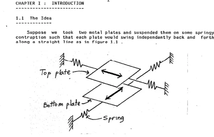
Suppose we took two metal plates and suspended them on some springy contraption such that each plate would swing independantly back and forth along a straight line as in figure 1.1 .
figure 1.1 : Two independantly suspended plates with perpendicular axes of motion.
Each plate has an actuator, in the form of a linear motor. Applying current to the motor will set the plate into motion, the pattern of which will depend on the physical characteristics of the plate and springs and on the input function. Specifically, if we apply a sinusoidal input to the motor, the plate will start oscillating back and forth.
If we oscillate the plates at different frequencies, such that one oscillates in a very high frequency relative to the other, then each point on one plate effectively raster scans the entire other plate.
If we mount a light pen with a very narrow beam in the center of the bottom plate and draw a grid on the top plate and then force the plates to oscillate as previously described, the light pen would trace a pattern on the top plate as in figure 1.2 :
y
[image:3.612.75.502.56.328.2]2
Now suppose we add a measurement device to our system. This device will give a real time measurement of the relative position of the two plates. If we replace the grid on the top plate with a piece of film and modulate the light pen by some logic coupled with the measurement device, then we can expose any pattern on the film, at will.
The most simple way to expose a picture would be to store the pixel image as a two dimensional array in the memory of a computer. The relative position of the plates, measured by our measurement device, is fod to the computer as X-Y coordinates and is used to fetch the corresponding pixel from memory. The computer can then decide on the modulation state of the light pen - on, off or anywhere in between, depending on the value of the pixel.
If we select a laser interferometer system as th~ measurement device, we gain extreme accuracy of measurement, way into the submicron range. The Laser Interferometer System has two more attractive properties : since tlie "meClsur· iny Ld1.n::" i:s d beclm or 1 iyhL, I.lie int.er-fenmc;t:t uf 1111:n;ha11 ic;:s dllLI measurement is kept down to practically zero. Also, a laser Interferometer System is perfect for relative position measurements.
If our mechanics are truly springy and flexible, then the motion of
the plates will be very smooth, free of bearing noise and backlash. Furthermore, we may use the Laser Interferometer System to enhance the accuracy of motion of the plates. By continuously comparing the actua1 position of the plates to the desired position, we can generate an error signal for use in a feedback loop to the linear motors.
A good application for such an accurate machine would be the making of reticles for the VLSI industry. A reticle is a magnified version of an actual silicon mask, where a magnification of 10X is common. In the current silicon technology the minimum width of a wire is about 5 micron, so for a magnification of lOX, the minimum feature size on film is 50
micron.
The film used for making reticles is a square glass plate, side. If we divide the film into 10,000 9rid 1ines per side, image will contain 10**8 pixels. Each pixe1 will be 10 microns correspond to an actual silicon area of 1 micron square.
3
1.2 Implementation
Implementing a machine as previously described incorporates four major tasks :
(1} Devising a viable mechanical design. The important requirements for such a design are stability and smoothness of motion. The accuracy of the mechanics is secondary, since we are hoping to achieve accuracy by employing feedback control. The mechanical design should also provide for coupling the machine with a
Laser Interferometer System.
(2) Designing a laser interferometer measurement device. This is the heart of the system. The final accuracy specification of the machine will be strongly related to the measurement error of the Laser Interferometer System. Here too we require stability of the Laser Interferometer System.
(3) Designing an exposure uriit . The requirem~rits for the exposure unit performence include a spot size of one pixel and speed of modulation and light intensity which are compatible with the speeds of oreration.
(4) Implementing feedback control for the system. If we require that our mechanics be simple enough to be treated by a mathematical model, preferably as a second order system, then our chances of conto11ing the machine improve.
At Caltech we have set out to design and build such a machine, which we call Flexigraph.
The Laser Interferometer System is based on a HP 5501-A laser transducer system. It employes a Helium-Neon laser with)\. =6329 Angstrem It has a resolution of approximatly 50 Angstrem and a measurement error of 0.5 ppm.
The amplifiers . in the servo loop are KEPCO bipolar operational power supplies model 36-5 M. This device has a frequency response of 20 kHz, and ripple and noise which are less than 0.01% of the maximum output.
The computer used to control the Flexigraph is a POP 11/34 with hardware multiply/divide and a floating point processor. The controllers run as stand alone code at a 10 KHz r~te. The computer 1s also equipcd with an ANALOGIC ANDS-5400 data acquisition system. This system has 12 bit O/A converters with accuracy and noise of 0.01% and a 10 micro second settling time for 1/2 LSB.
All Laser Interferometer System components were produced by milling nluminum 6061 on a computer controlled milling machine which is accurate to 0.005". The plane mirrors in particular were milled out of 1" sQuare aluminum 6061 bars. The reflective surfaces of the mirrors were produced
4
5 1.3 Specification
The Flexigraph prototype built at Caltech conforms to the following specifications :
MEASUREMENT ERROR
DEFORMATION ERROR
RESOLUTION
SERVO LOOP RATE MOTION DEVIATION
MAINTENANCE
1 part in 10**5.
3*10**-5 radian 6 seconds of arc). 5*10**-2 micron 5*10**-8 of a meter). 10 kH:z.
2 to 10 microns (0.2 to 1.0 micron on silicon). The Flexigraph prtotype has been in existance for over half a year, and though it has been appreciably abused, realignment or readjustment were not found necessary.
The remainder of this paper details each of the major implementation tasks enumerated above and discusses results obtained when testing the prototype machine.
Chapter II describes the mechanical design of the Flexigraph. Chapter III describes the Laser Interferometer System and gives an analysis of the measurement error.
6
1.4 Related Documentation
7
CHAPTER II : THE MECHANICAL SYSTEM
2.1 Mechanical Description
The basic concepts of motion of the Flexigraph are best illustrated
by the following top v1ew drawing :
CD
h
-
.x
·~©
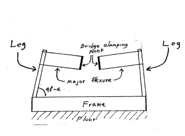
figure 2.1 : A top view of a carrier plate suspended on four major f1exures. The plate can swing back and forth in the·v direction. A bridge like structure is suspended on four major flexures at (1), which in turn are suspended on four legs at their other edge at (2). The
legs extend downwards and attach to a frame supported by the floor.
Each flexure has two vertical grooves milled in it as demonstrated in figure 2.5. These grooves serve as pivots when the flexure is bent sideways. The location of these grooves is denoted in figure 2.1 by small triangles.
The bridge is not rigid, but rather consists of two tuning forks clamped back to back, thus creating a carrier plate at the center of the structure. The arms of the tuning forks serve as minor flexures which can bend outwards or inwards.
If we try moving the bridge in figure 2.1 in the Y direction, the four major flexures will bend and their inner edges, that is the edges to which the bridge is attached, will move along an arc as seen in figure 2.2
... ...
...
+---...wit~
L
eJ
8
When the bridge moves in the Y direction, the distance between the odgos of oach major floxuro pair incroasos, duo to tho arcs in which they travel. To accomodate this increased distance, the arms of the tuning forks must bend outwards, thereby generating an inward retaining force. This force adds to the retaining force of the major flexures, with the net result being a spring like action which tends to center the bridge.
The geometry of the Flexigraph when the bridge is displaced from its resting position is illustrated in figure 2.3.
Le_J
}'\inor-
ye~1Ji!IV'j ~rce
M
G\j orrelrA.1
n
IJl\j
:fon:.
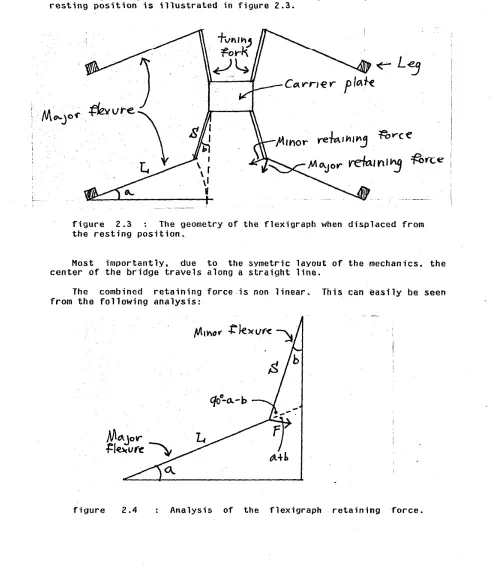
e :figure 2.3 The geometry of the flexigraph when displaced from the resting position.
Most importantly. due to the svmetric layout of the mechanics. the center of the bridge travels along a straight line.
[image:10.612.58.556.163.731.2]The combined retaining force is non linear. This can easily be seen from the following analysis:
9
The tuning fork exerts a force perpendicular to the minor flcx11res. The component of this force which adds to the retaining force is F*sin(a+b). In other words, the further the system is from its resting point, a+b becomes larger and a greater percentege of the force in the minor flexure is converted into a retaining force. Moreover, the minor flexure force itself is proportional to the square of the displacement of the bridge because the fork is deflected by the amount by which the circular swing of the major flexure differs from a straight line.
Putting all this together, the main retaining force on the moving bridge is proportional to the cube of the bridge displacement.
10
2.2 Flexure Analysis
Imagine a flexible hinge as shown in figure 2.5. This is a drawing of a major flexure made of aluminum sheet. To get long fatigue life from aluminum, the stress within the flexure should not exceed 7000 PSI. Youngs modulus for aluminum is 10,000,000 PSI. Thus the maximum tolerable strain
is 7000/10**8 = 0.001
Consequently, if we restrict the deformation of the flexure down to one part in 1000, we can expect a reasonable fatigue life. A deformation of 1 ~ 1000 also establishes the minimum permissible L/T ratio for a given deflection angle
e.
When the flexure is curved, its outer cord is longer than 1ts 1nner cord by r~e and the stra1n 1s s=
(T~e)/2L . Tne factor or two comes in because the outer cord lengthens and the inner cord shortens. Thus for a flexure of approximatly 50 cm and a film of 10 cm, the bend will be 5/50 = 10% ore
=
0.1 radian which is about 6 degrees. We must therfore have L/T=
0/(2*S)=
0.1/(2*10**-3)=
50:1.f1gure 2.5 ana1ys1s of a bending flexure. Note the groove in the flexure which serves as a pivot.
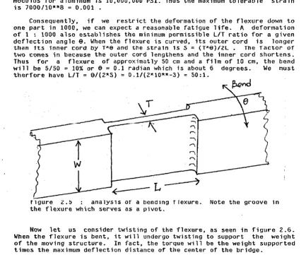
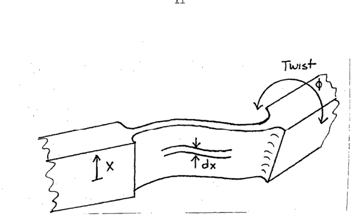
Now let us consider twisting of the flexure, as seen in figure 2.6. When the flexure is bent, it will undergo twisting to support the weight of the moving structure. In fact, the torque will be the weight supported times the maximum deflection distance of the center of the bridge.
The torque provided by an incremental flexure dX, is proportional to X**2 because parts of the flexure farther from its center are deflected
farther and thus not only provide more force but also have a greater
moment arm. The total torque developed is the integral of the incremental torques ,
r
=
r
t1i11i
K.fxi.
JJc
J ...
~1z
( 1) [image:12.614.88.522.147.509.2]11
figure 2.6 Analysis of a twisting flexure. the twisting is due
[image:13.612.114.466.83.300.2]12
2.3 Z Axis Alignment
The torsional force in the flexure may cause dipping of the bridge as
it travels. thus causing l axis misalignments. There is a neat solution to this problem. If the flexures are clamped to the frame at an· angle to the floor, as illustrated in figure 2.7, then the plane of motion of the flexu.res is also at an angle to the floor. This means that as the bridge is deflected from its rest position, the flexures tend to "climb up", thus
compensating fo1- torsiona.1 dippin9 of the bridge.
[image:14.612.126.488.197.464.2]13 2.4 Momentum Conservation
When the bridge is set into motion, momentum conservation applies. This means that whenever the bridge moves in one direction, the frame will tond to move in the opposite direction in order to to maintain zero momentum for the system as a whole. In order to isolate the frame from this unwanted motion, a secondary contraption is added to the system. It
is clamped to the flexures as illustrated in figure Z.8 :
Sc!4cnd~r; confro.ffto~
~~~~~J
figure 2.8 : The modified version of the flexigraph with an added contraption to balance the momentum.
The major change to the original bridge is that the flexure is no longer clampped to the leg of the frame at its end, but rather somewhere in the middle of the flexure. Each flexure has now become a double flexure. When the bridge moves in one direction, the secondary contraption moves in the opposite direction to balance the momentum. This is because the linear motor is attached to the bridge at one end and to the secondary contraption at the other end.
If the ratio of lengths of the two parts of the flexure, shown as b/a in figure 2.8, is set to be equal to the ratio of the bridge mass to the secondary contraption mass, then the clamping points of the legs remain stationary while the other parts are moving, and the frame is virtually isolated from the motion. We can contr-ol the length ratio by moving the clamping point of the leg, or we can vary the mass ratio by adding weight to either of the two parts.
This design change also provides an elegant solution as to where the linear motors are positiond. As can ,be seen in figure 2.8, the permanent magnet of the linar motor is attached to the secondary contraption, while the coil is attached to the center of the bridge.
14 2.5 Flexigraph Setup
By
taking two units as described previously, and mounting them one above the other and perpendicular to each other, we obtain a system withtwo perpendicular axes of motion_ The two units are mounted on the same
frame, but if the momentum balancing alignment is performed carefully, the frame should be isolated from vibrations deriving f rom the motion of either axis.
15
2.6 Summary
The proposed mechanical design provides for:
1) An oscillatory motion along a straight 1ine. The motion is very
smooth and free of bearing noise and backlash.
2} A retaining force which increases rapidly when the bridge approches its end of travel.
3} Decoupling of the frame from vibrations generated by bridge motion.
16
CHAPTER III : THE MEASUREMENT SYSTEM
3.1 Definitions
oe-Y '"
f
er:f'en:i111efer
:~
Y
/~sef'
t:Ji..xts·:
1~Y ~'"or
Y
Mlf"V"~r 0-..'XIS.y
'
[image:18.612.60.565.43.625.2]Lx
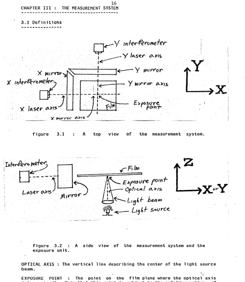
figure 3.1
A
top view of the measurement system.figure 3.2 exposure unit.
z
A side view of the measurement system and the
OPTICAL AXIS : The vertical line describing the center of the light source beam.
1/
CENTER OF FILM : The exposure point when a11 flexures are at their rest position.
FILM PLANE :
Plane of film surface.MOTION AXES
ana Y briage. The geometric lines describing the motion of the X bridge MOTION PLANE The plane which passes through center of film and is parallel to bcith the motion axes. In other words, the motion plane describes the motion of center of film.
MIRROR AXES : The geometric lines normal to the mirror surfaces.
MIRROR PLANE The plane which passes through center of film and is parallel to both the mirror axes.
LASER AXES : The geometric lines describing the segments of 1a5er bedm
from the interferometer to the mirrors.
LASER PLANE : The plane which passes through center of film and is
18
3.2 Ideal Alignment
Under conditions of ideal alignment, the following statements hold true :
1) The film plane, motion plane, mirror plane and laser plane, all exist and coincide.
2) The mirror axes are perpendicular to each other.
3) The laser axes are respectively perpendicular to the mirror surfaces.
4) The laser axes intersect at the exposure point.
Misalignments may be internal to the measurement system, as when some components are permanently displaced from their ideal position, or may be due to external forces rising from non linearity in the motion of the bridges. Not all misalignments will introduce errors. For example, if
the four planes do not coincide but are still parallel, no error will result.
19 3.3 Motion Misalignments
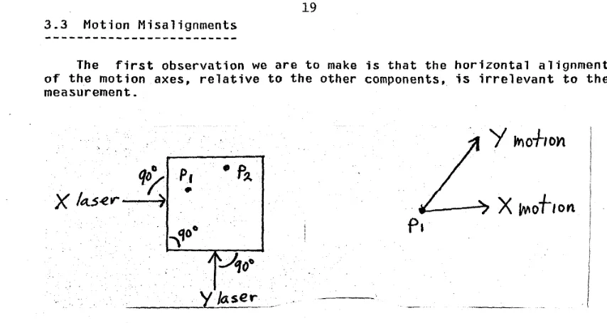
The first observation we are to make is that the horizontal alignment of the motion axes, relative to the other components, is irrelevant to the measurement.
P1
•
•
p~y
/a.ser
) Y
11iOf1on
.Lx~ofron
[image:21.612.75.502.78.305.2]P•
figure 3.3 : Analysis of motion misalignments.
We illustrate this point by applying some arbitrary motion vectors. X motion, Y motion and noting that the exposure point has moved from Pl to P2. The laser Interferometer System can be regarded as an analog computer, which performs a vectorial sum of the motion vectors and transforms this vectorial sum to the mirror coordinate system. Since only the vectorial sum is relevant, the Laser Interferometer System will measure correctly regardless of the alignment of the motion axes.
The same argument may be extended to deal with the case of bridge
motion which doos not follow a straight ling, As long as thgro is no
relative rotation between the mirrors and the laser axes, our analog computer model holds.
However, two types of errors may result from non linear bridge motion. First, if the motion deviation is along the Z axis, this will cause the distance from the light source to the film to change, thus affecting depth of .focus.
20 3.4 Film Misalignments
We shall start with the case of the film not being parallel to the laser plane as shown in figure 3.4 :
Lo.~er Q..X/s
>
figure 3.4 Side view of a system with the film plane not ptu-allel t.o th1:1 mea::.ur-ement pldlltt.
This has two effects : If the film plane is not parallel to the motion plane, then the depth of focus will be affected. This misalignment will not be treated in the current analysis. The second effect is a cosine error resulting from the fact that the measured distance and true distance do not coincide, as illustrated by figure 3.5 :
La.se
rf
/drie,I
I
21
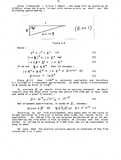
Since X-measured X-true ~ COS(a) • the image will be scaled up by
1/COS(a) along the X-axis. To deal with cosine errors, we shall use the
following approximation :
figure 3.6 Hence
x
2=
1
2 .,.e'.2..
"""">
(l+5)
4=
I+
E..
1t>
I
+
2.j
+
~t...-=
I
-t
c.:~-I f we set ~ -::::::.
Jz..
€. 1... then ( 3) becomes( e
<<
I)
(1)
(2)
(3)
I
+
e:
2+
~
c...
=
I
+
e
7.+
£
rY"O r=>
(
4) (5)Since E «1 then . 1/4E"i is certainly negligible and therefore
X ; 1+1/2€i is a reasonable approximation. In other words, a displacement of E causes an error of 1 /2
ez. .
To evaluate
£
we should ·first set an accuracy standard. We shall require that the total error across the entire film (100 mm) is less than one tenth of a pixel (1 micron) :<!. _,
I _,
~ : 10 W'1 ID Iii\
=
(6)Our alignment specification, in terms of
!:,. ,
becomes :Error<
S
->
Jz.
E~S'
=/
e<
S"°' 10-3<n
Returning to our film misalignment, this means that if the ratio of height deviation to rilm size is better than l/ZOO, the cosine error 1s negligible. On 100 mm film, we can tolerate deviations of up to 1/2 mm. Considering the film plate is flat to within 28 microns and the plate holder is milled to an accuracy of 0.005 inch, the 1/2 mm requirement is easy to meet.
[image:23.612.55.555.70.727.2]22
Rotation around Z axis will merely displace the image on the film. We
not~ hnwevRr that X,Y or 7 rntRtion~ hehRVP riifferently when rlue to
dynamic non linearities. For one thing, they involve mirror rotations as well, since the film and mirrors are rigidly connected. In any case,
these errors are treated later on.
23 3.5 Laser Misalignments
There are two classes of laser misalignment : the first class contains severe misalignments resulting in the deflection of the returned laser beam to such a degree, that it misses (or nearly misses) the detector. If
detection is broken, The Laser Interferometer System stops the measurement automatically and reports the problem.
fhe second class involves all misalignments which do not interfere with continuous detection.
We
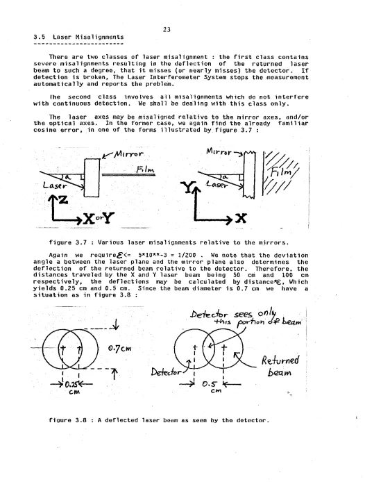
shall be dealing with this class only.The laser axes may be misaligned relative to the mirror axes, and/or the optical axes. In the former case, we again find the already familiar cosine error, in one of the forms illustrated by figure 3.7
·'J'Z. · ..
[image:25.612.59.585.40.734.2]..
·Ltx
0
~Y
figure 3.7 : Various laser misalignments relative to the mjrrors. Again we require~<= 5*10**-3 = 1/200 . We note that the deviation angle a between the laser plane and the mirror plane also determines the deflection of the returned beam relative to the detector. Therefore. the distances traveled by the X and Y laser beam being 50 cm and 100 cm respectively, the deflections may be calculated by distance'\£,, Which yields 0.25 cm and 0.5 cm. Since the beam diameter is 0.7
cm
we have a situation as in figure 3.8 :J:>e-fe.c./r:,r
:sees.
o~
16/ .
·)
+his.
f'>.rno111
c!:P
.b.ettm \
!
I --:-it\
. f
I
-.::f.o.~
CM
24
Concentrating on the right part of figure 3.8, we notice it is on the verge of detection being broken, since the detector must recieve at least 20% of the original beam. We assert then that by virtue of having a continuous detection, the cosine error resulting from laser-mirror misalignment is negligible.
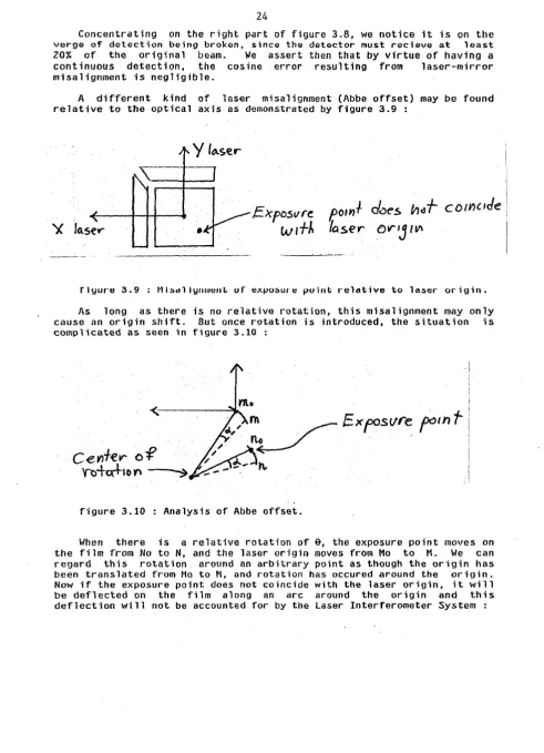
A different kind of laser misalignment (Abbe offset) may be found relative to the optical axis as demonstrated by figure 3.9 :
Y
l~ser
•
Expos11re
w1+A
eom+
d::Jes
l!Jdf
com<.1de
laser
O~'j
IV\flyure 3.9 : Ml~dl1ynment of e~posure point relative to laser origin.
As long as there is no relative rotation, this misalignment may only cause an origin shift. But once rotation is introduced, the situation is complicated as seen in figure 3.10 :
Cenf-ev-
of
Yb+c.r+-tof\
~
figure 3.10 : Analysis of Abbe offset.
[image:26.614.59.550.62.740.2]25
f01Y1
t
figure 3.11 : Analysis of Abbe offset.
If the distance between the laser origin and the exposure point is 0, then the deflection equals 0*9 . Let us examine
e.
Rotation of thebridges during motion may result from a sudden "jump" or from mechanical
inaccuracies. Jumps will tend to spend most their energy on X-Y translations which are unrestrained. Their contribution to rotation will be small due to the rigidity of the bridge-frame connection. Mechanical inaccuracies, especially those due to flexures of unequal length, will rotate the bridge as seen in figure 3.12 :
i
.De~
I
e.
c+um.. ().
"J
k
0f->
br-1d9e
[image:27.612.60.542.45.680.2] [image:27.612.108.516.50.252.2]26
When the flexures are bent to angles &1 and 62 , the center of the bridge is deflected from G to F , due to Xl being uneQual to X2 :
x,:::.
R
1
(I -
cos e1)
x
2=-
Ri
Cf
-Co~ ~l)
(S)£=
('X,-Xl..)/2
::::'
(R,
(!-CDS,$,) -Rt.(l-{0$6-J)/2<0)
Now 91
=
dl/Rl=
(1/2 film size)/Rl=
5 cm/50 cm= 1/10 radian. for such angles' we might as well take 01 = 92 .=e,
and (9) becomes :E.-=
(R,-Ri)(/-CoS$)/;;...
(10)The angle o{ is determined by : cl.= 2*E/L where L is the bridge length,
l 100 cm therefore :
d.::
(R,-R
1 )(1-.q,s)/foD
=
(R,-Ri)·S./0-s
(11)Even if we take R1-R2 to be as big as 1 cm,
cX
will be as small as5ft10**-5 radians ! Returning to our misaligned exposure point, we get
·Error-:::
D~ol
=>
D
=
10-~/S·lo·S'=".2
cw.
c12)It seems we need not be too concerned about unequal flexures. However, rotation of the bridge can also be caused by unequal spring
constants in the arms of the tuning forks, as demonstrated by the following figure :
; I
¥i
'
I
-++-
.'
[image:28.612.76.569.78.597.2]I '
27
Now the deflection angle 0( is given by
~
= (
<l>2 -
cp
I )I
.2.
(13)In the worst case. Kl
>>
K2 and hence 01>>
02. Applynig this to (13) we get°'
=
tj,_/1..
=
¢::
d/r..,
=
R (t-cos6)/L,
-=>
(14)c;;.
=
SOc
m(I - . 'MS)/
SOc
~-::
O • O OS ru.d 1 a., (15)assignig this value of worst case d_ into (12) we get .:
28
3.6 Mirror Misalignments
Rotations of
the
mirrors aroundX,Y
orZ
axeswill
cause cosine errors dependent on the angle of rotation. As we have seen in theprevious
section, this angle is extremely smn11. Unsurprisingly, translations in
X,Y and Z introduce no errors. Nevertheless, it is the mirrors which introduce the most severe error in the system. This happens when the mirrors are not perpendicular to each other, as in figure 3.13 :
. Y
/<>..s-er
- i
figure 3.13 Deformed geometry caused by non perpendicular mirrors. This will cause the geometry on the film to be deformed such that rectangles will appear as parallelograms. The problem is, we are faced with a sine error, since maximum deviation equals (film size)*SIN(a). Because for small angles SIN(a)
=
a. the error is no longer negliaible- a deviation oft causes an error· offand not 1/2cuz as was the case for a cosine error. In other words, in order to keep our standardsS
>
Errcir
->
S
>
6
=o<=>
cl<
10-sr"'d'"'n.
(13)29
3.7 Variable Cosine Errors
Cosine errors scale the image up or down, depending on the specifics of the misalignment. When cosine errors are constant, due to permanent misalignment, the scaling is constant, all proportions are preserved and
unless we measure the dimensions of the image, we will notice no
deformation.
However, when a cosine error is a result of a dynamic misalignment, such as rotation during motion, the angle of deviation will most likely be a· function of X and Y. as a result, distinct regions of the image will be scaled differently, and non linear deformations will be found.
Suppose the bridge dips as it travels. Looking at it from the side we could see :
F1IW'
figure 3.14 Dipping of film as a result of non linear bridge motion.
This is an exaggerated diagram. The center of film is actually limited to move only between the two small arrows. Such a journey would result in a true grid appearing on film as one of the following :
Otae
o..)(tsscale
vp:
·fl>lo
·~scal-e
ur:
figure 3.15
TwO U\XeS
scale
ciolm!:
r---1=~:t::t--t---t
[image:31.612.47.550.219.642.2]30
A different kind of deformation may be found as a result of a sudden jump, caused by backlash in the system. Suppose a bridge, when seen from above. performs such a jump !
· tco
figure 3.16
Since the mirrors are rigidly connected. a scaling of both axes will occure between Yo and Yl, and a true grid will appear on film as seen in figure 3.17 :
[image:32.612.79.571.73.745.2]y,
31
A similar deformation will be found if the light source suddenly drifts. resulting in an unaccounted for motion of the exposure ooint. as
[image:33.612.52.577.105.714.2]seen in figure 3.18 :
figure 3.18 : An image shearing effect caused by light source drift. The difference between the last two cases is that for a light pen drift the scaling is the same on both sides of the deformation region-only an image shearing effect is found.
The deformations appearing in figures 3.15-3.18 look quite discouraging. The drawings themselvs have in fact been quite exaggerated. In reality, our 10**-5 accuracy standard guarantees a maximum deformation, across the entire film, of less than 1 micron. In other words, the
measurement error of the Laser Interferometer System is on the ur~cr
or
132
3.8 Summary Of Errors
We have seen three types of errors :
COSINE ERROR : Due to permanent or transient misalignments. The permanent cosine error fs limited to 1 micron over the entire film by virtue of having continuous detection. The transient cosine error is much smaller than the permanent one, since the angle of rotation of the bridge is limited by the geomtry and rigidity of the machine. Permanent cosine errors will cause. image scaling, while transient cosine errors will cause image deformation as well.
SINE ERROR : Due to mirrors not being perpendicular to each other. This error will cause geometry deformation. In order for this error to be less than 1 micron over the entire film, the mirrors should be aligned to within 2 seconds of arc.
ABBE OFFSET Oue to the exposure point not coinciding with the laser
33
3.9 Alignment Routine Outlines
Based on the error analysis presented in this chapter, the following steps were taken to align the Flexigraph :
1) Using an optical bench, an autocollimator and two precision cube corner references, the mirrors were aligned to be perpendicular to each other. The alignment apperatus is diagrammed in figure 3.19. The autocollimator and cube corners each have a specified accuracy of 2 seconds of arc. The axes deformation is therefore 6 seconds of arc, or 3*10**-5 radian.
[image:35.612.64.581.69.701.2]Mirrors
figure 3.19 : Mirror alignment apperatus using an autocollimator and two cube corners.
2) Using a distant wall as a target, all laser bed components (laser
head, beam splitter, beam bender) were 6ligned to produce two parallel beams as illustrated by figure 3.20. The accuracy of this alignment is 1 : 10,000 or 2*10**-4 radian. Note ·that the previous cosine error analysis requires an accuracy of 1 : 200 on·1y.
Beam
·
b~VJ<lerJ
L.~~
E>eo.WJ
spl~r
figure 3.20 beams.
34
3) The brirlges were alioned, leveled and balanced by mechanical means
to produce as smooth a motion as posible.
4) The plate holder was mounted on the Y bridge and the light source support on the X bridge. Using a precision flat plate and a dial indicator, the film plane was aligned to be parallel to the motion plane.
5) The 1 ct::.er- l.itnl wets muunteu on the frame. Using autorefl ect 1 on on
the X beam and passing through a height target with the Y beam, the laser bed was aligned, as illustrated by figure 3.21
~ .c__~~-
L
3
·1f-;.~~.
.__:_:_'X-..:!::b:.::::=;.e~~IM -*-A~,'/---)
fr.v.f.o'fi:#/.ec.:fton
t
M\f(Of"Sfigure 3.21 Alignment of laser bed relative to the mirrors.
6) lhe X 1nterterometer was mounted and aligned using the HP target.
[image:36.612.55.563.69.740.2]35
CHAPTER IV : THE EXPOSURE UNIT
4.1 Exposure Unit Requirements
The exposure unit consists of a light pen and a film plate. The light pen is mounted on the bottom carrier plate of the Flexigraph and the film on the top plate. By oscillating the top plate and advancing the bottom plate slowly, the light pen raster scans the film. There are 10,000 scan lines over a film of 10 cm. Thus for an oscillation frequency of 1 Hz, the exposure time for a 10 micron pixel is 10 micro seconds.
The requirements for the light source are therefore : 1) Spot size of 10 microns.
2) Exposure time of less than 10 micro seconds. 3) Modulation speed on the order of 1 micro second.
The requirements for the film are :
1) High rP.solution.
2) Flatness.
3) Cleanliness.
4) Film sensitivity which is compatible with the speed of operation of the Flexigraph.
The film we chose to work with is KODAK high resolutin plate type 1-A. The resolving power of this film is better than 2000 lines per mm. or 20 lines per pixel. The flatness of the plate is specified such that all points on the glass surface beneath the emulsion lie between two parallel planes separated by 28 microns. The plate also has an anti halating backing and is ultrasonically cleaned prior to packaging. The spectral sensitivity curve of the film is shown in figure 4.1.
lo....-~~...-~~ ... ~~--.,r--~---r
(
J - ICOOAr: Hlo~ •••• r ... ;_ rr ... T1..- ::IA
.t.Ol--~~-4-~~--+~~~-i-~-:---t
figure 4.1 : Spectral sensitivity curve for type 1-A plates.
Unfortunately the emulsion Of1 these plates is extremely slow.
However, since these are the only commercialy available plates that
[image:37.614.80.520.294.606.2]36 4.2 The Light Pen
It had been proposed to use an LEO as the light pen of the Flexigraph, the argument being that since a pixel is so small, the amount of light required to expose it must also be small. Therefore, provided the film is
sensitive enough, an LED should do the job.
To verify this point we carried out a few experiments using a green LED since the type 1-A plates are most sensitive to green light, as can be seen from figure 4.1 . Incidently, the film is not sensitive at all to the red light of the Helium-Neon laser.
The first experiment was to test the spot size produced by an LED when focused through a microscope, as in the following set up :
Gtreen
··LED
figure 4.2 : An exposure experiment to determine the minimum spot size which can be achieved by focusing an LED trough a microscope.
This experiment yielded spots of 40 micron on film. Since the set up was very crude, it seems that 10 micron spots are easily obtainable.
[image:38.612.79.530.215.518.2]37
LED
.-.
figure 4.3 : An exposure experiment to determine minimum exposure times for an LED using type 1-A plates.
Driving the LEO with a 60 mA current, the minimum exposure time was established at 5 seconds. Since this result is 5 orders of magnitude too slow, we clearly face a problem.
We now have two possibilities
1) Increasing the sensitivity of the plates. 2) Increasing the intensity of the light pen.
As mentioned previously, the type 1-A plates are the only plates of this class which are commercialy available. It seems therefore that our only resort is to find a stronger light source. Perhaps the best solution
is to use a green laser, since lasers arc compatible with the required
[image:39.614.78.483.118.267.2]38
4.3 Summary
1) The film selected for the Flexigraph is the KODAK high resolution plate type 1-A. These plates are commercialy available and fill all requirements of resolution, flatness and cleanliness. However, the emulsion of the plates is very slow.
CHAPTER V : THE CONTROL SYSTEM 39
5.1 Mathematical Model
The flexigraph is charcterized mechanically by the presence of inertia (mass), stiffness and viscous damping (the major and minor flexures),
shown schematically in figure 5.1 :
Flt)
)
M
cj,_Fc_<:J
-- -- -- --
c:
figure 5.1 : Modeling of the flexigraph as a second order system. By Newtons second law of motion :
Flt).-
Fs
(t) -Fc:J(t)
=
M~
Since Fs
=
-KX and · Fd=
-CV by assignment we getF(t)-=
M~
+Cit+
K}('
Systems described by such an equation are generally Second Order Systems. A more convenient form
or
(Z) 1s :Where factor.
-X
+
2
~
wh
x
+
w~
x
=
Wk
F(J;)
Wn
~ is the natural frequency, and ~(1)
(2)
ref ered to as
(3)
is the damping
We can gain substantial mathematical insight into the behaviour of a system by working with the transfer function of the system. The transfer function is defined as the ratio of the Laplace transform of the output to the Laplace transform of the input, with initial conditions equal to zero. The Laplace transform of (3) is :
where X(s) is the Laplace transform of the output
the Laplace transform of the input F(t). The transfer
definition
We can write the output response of a system as: X(s)
=
G(s) ~ F(s)(4)
X(t) and F(s) is
function is by
(5)
[image:41.612.70.534.61.725.2]40
In other words, the output X(s) is dependant on the input F(s) and on the physical characteristics of the system, lumped into G(s). In an ideal system we would like X(s) to depend only on the input F(s) and keep the machine interference G(s) to a minimum. The fact is that physical systems do interfere with their surroundings and that in the real world G(s) never reduces to the unity functinn_
G(s) is unique. For a given system, there is only one transfer function. The question is, how do we arrive at G(s) ? Given that the input function F(t) is the impulse function
cf".
by definition F{s)=
1 . Assigning into (6) we get :X~)
.s"+
z.5w"
s.
+
W...-i'l..In other words, we can hit the system with an impulse output.response. This response is the transfer function.
( 7) and r:ecord the
The quadratic equation S'2-t.iSw.,.stWl·= o 1s called the characteristic eqution. It has two roots in the complex plane since S, introduced by the Laplace transform, is a complex variable. By definition, these roots are also the poles of the system. The location of the system poles in the complex plane has a strong relationship with the transient time response of the system.
The poles, being complex numbers, have a real part s and an imaginary part jw. Moving a pole of a system along the real axis will change the decay rate of the system response. The more negative s becomes, the faster the decay rate. For s ~ 0 there is no decay, and positive real parts are associated with unstable systems in which the output increases without limit, as seen in figure 5.2. However, for second order systems, the real parts of the roots are always negative, as can be seen in (8) .
w
s<<O
S-=o
S>o
s~>ofigure 5.2 : The decay rate as a function of s, the real part of a
system pole.
[image:42.612.81.547.404.559.2]41
.·.· .-d\
JW
1ncvea~
figure 5.3 : The frequency as of a system pole.
f
_ /
~
-- ia function of jw, the imaginary part
For a second order system such as the Flexigraph, there are two poles of the form:
(S)
The magnitude of the imaginary part Of the poles is
w-:Wn VJ-.JL.
This term is called the damped natural frequency of the system. It is the frequency of the actual oscillations of the system.For a given
Wn,
ifO<! <1
thenWi
0
and the system is under damped andwill oscillate. If~= 1 then l.V= 0 and the system is critically damped
and will not oscillate. if}>1 then the system is over damped and will not oscillate. Typical time responses of second order systems as a function of~
[image:43.612.68.552.47.686.2]are illustrated in figure 5.4 :
42
A typical root locus plot for a second order system as a function of
C:-is prgsented here as
fiour~
5_5 :~
[image:44.621.49.564.85.710.2]43
5.2 Charcterization Of The Flexigraph
How far is the Flexigraph from an ideal second order system ? A good 1nitial indication may be obtained by taking time response snap shots of the system and comparing them to the model. It is easiest to apply an impulse input to the system because when the forcing term F(t} is an impulse, its Laplace transform is F(s)=l and the transfer function G{s):X(s)/F(s) reduces to G(s)=X(s).
The time response of the Flexigraph to an impulse input is shown in plots 1,2 and 3. The dominant effect in plots 1 and 2 is an underdamped second order system withW of the order of 1 Hz. On it is super imposed a
second oscillat1on of about 5 Hz with a much smaller amplitude and a damping factor which is close to zero. A blowup of this oscillation is shown in plot 3.
The 5 Hz oscillation is obviously not part of the desired system. It must be due to effects not accounted for by our model. After some experimentation with the Flexigraph, the source of this oscillation was discovered. Whenever excited with a 5 Hz input the system would beoin to shake vigorously making it visually apparent that the legs of the frame were the cause. It seems the true model for the Flexigraph is our previous second order system, mounted on an inverted pendulum. as seen in f'igure 5.6 :
K
c
~~~--~--'""'v"-~~--~./
J=.
l.e
)C,9
v-111.ph
L
r
()\f .(V"+u1f€nclvf
"~
1figure 5.6 Modeling the flexigraph as a second order system mounted on an inverted pendulum.
The 5 Hz oscillation appe~ring in the plots is the oscillation of the pendulum.
[image:45.612.156.462.336.510.2]44
5.3 Structure Changes
The structure of the legs was changed in order to cancel, or at least dampen the legs' vibration. Dampers were added between each pair of opposing legs, via an added support structure as drawn below :
©
figure 5.7 The support structure added to the flexigraph to eliminate the leg vibration.
Rubber dampers were inserted at all point of connection between the supports and the legs, denoted by (1) in figure 5.7
The time response snaps were repeated, and are presented in plots 4,5 and 6.
Plot 4 shows the time response of the modified Flexigraph to two different inputs- an impulse input and a step input. It is clear from the plot that the situation has improved dramatically but the problem does persist to some degree, as the blowups io plots 5 and 6 clearly show.
45
5.4 Error Signal
It has been previously shown that the output of a system X(s) is dependant on G(s) and on F(s), the Laplace transform of the input F(t). What will F(t) look likA in the working environment of the FlexigrRph ?
It was decided to operate the Flexigraph as a raster scan generator. This means that one axis will be made to swing back and forth by applying an oscillatory input signal into its linear motor. During each oscillation the film will sweep once across the exposure unit, thus potentially exposing one grid line on the film. The second axis of ~he Flexigraph is made to move very ~lowly in one direction, thus advancing the exposure unit from one grid line to the next.
The frequency of the oscillating axis is limited by the maximum velocity allowed by the laser interferometer system which is 6 in/sec. Since this comes out close to the natural frequncy of the Flexigraph, i t was decided to oscillate the system at a frequency of 1 Hz.
What kind of error signa1 will be produced by oscillating one of the Flexigraph axes ? The error is due to the motion axis and the measurement axis not being aligned as shown in fig 5.8:
figure 5.8
[image:47.614.79.555.140.690.2]46
t-::.o
figure 5.9 When the measurement and motion axes perpendicular a stationary interferometer will notice a distance to a sweeping mirror.
are not changing
[image:48.615.58.548.58.393.2]47
5.5 Frequency Response
Since we are dealing with an oscillatory error, it is important for us to examine the frequency response of the Flexigraph. By applying a sinusoidal input with a varying freauency to the linear motor. the magnitude and phase shift of the output are recorded to produce a polar representation of the frequency response, given in plot 8. This plot is the frequency response of the flexigraph around the resting position, with all flexures in)tially at zero deflection.
[image:49.612.69.530.57.758.2]Typical plots for a second order system as a function of the damping factor·.5 are illustrated in figure 5.10 :
figure 5.10 : Typical time response plots for second order systems.
An examinat1on or ploL 8 reveals a natural frequency at 0.85 Hz. Its presence is signaled by the bulge of the outline, representing a maximum point on the magnitude scale. The difference in frequency from a natural frequency of 1 Hz to 0.85 Hz is due to plots 1-6 being of the mechanical system only. while the frequncy response in plot 8 being of the mechanical system and linear motor as well.
In fact, the effect of the linear motors is clearly evident in the damping they contribute to the system. Jf we simply short circuit the motors and try to deflect the bridge by manually pushing it, a considerable resistance is created by the coils. This damping can be seen in plot 8 by the fact that the magnitude of the response at the natural frequency point is only 2.0.
Somewhere between a frequency of 1.4 Hz and 2.0 Hz occurs the breakoff point of 3 Db, recognized in plot 8 by a magnitude of less than 0.707. We ·also notice that for frequencies above 3.0 Hz the phase shift is practically 180 degrees and the magnitude is nill.
48
5.6 Closed Loop Experiments
The most simple and obvious way to apply feedback control to a system is by using a proportional controller as shown in block diagram in figure 5 .11 :
Error
t=.~J
rt~><i~ro.J>~
6-~)
...
___
__,..,,
Aw.rM1~,.
--~~~
K
...--~~~~--figure 5.11 : A block diagram of a proportional controller.
OvTJVT
X~J
The reference input is constant, since we want a straight line, and may be taken for convenience as zero. We are simply feeding the linear motor with an amplified version of the e~ror sinusoid.
The results of applying such a controller to the Flexigraph are shown in plots 9,10 and 11.
Plot 9 shows an uncontrolled error signal (open loop) with an amplitude of 40 micron. Superimposed on it is plotted the same signal when the proportional controller is applied. We can see that the error has been improved to slightly better than 50%.
In plot 11 we see the same controller with a higher gain. The open loop error signal in this case is 60 micron and it is reduced to approx 18 micron, an improvement of 70~.
[image:50.612.92.509.136.362.2]49
Rc.s)>--~
I
6-<?)
XCsJ
figure 5.12 A block diagram of a proportional-derivative controller.
The reference signal is again kept at zero and the linear motor is fed with
an
amplified version of the positional error and the velocity error. In this case we are penalizing the system for developing any velocity, since the reference is zero.The results obtained with this controller are shown in plot 11. For an open loop error of 60 micron, the controller has generated a straight line to within 5 microns. A closer look will reveal two more interesting facts.
The first is that the Flexigraph has some instability, since the closed loop error is better than 2 micron for the first four seconds of operation and increases to about 5 microns thereafter. We may also note a slow climb in the graph for the first few seconds. This is due to initial conditions which are overcome slowly due to a large gain used for the velocity Arror.
1he second fact to note is that most of the remaining error is a sinusoid of approximatly 10 Hz. It is obviously an occurance of leg vibration. The fact that the frequency of the leg vibration is changing all the time, from 5 Hz to 8 Hz and now to 10 Hz is not surprising, since applying a controller changes the system. and is very likly to shift any of the natural frequencies. This effect is well demonstrated when comparing plots 2, 4 and 10. These plots are all impulse responses of the
same system, but the difference in system parameters produces different
natural frequencies.
Wevei-theless the results tu-e good. Even without. e11ha11ci11g sl.dl.iilit.y,
a 5 micron error on film means a 0.5 micron error on silicon, since the reticles are exposed at a magnification of tOX. Improving the stability of the F1exigraph seems to promise reducing of the error to 0.2 micron on
silicon.
The results discussed so far were obtained for a limited film sweep of
approximat ly 20 mm. How wi 11 the Flexigraph behave if we try to expose
50
In plot 12 we see an open loop error of 200 micron. Superimposed on
i t is plated the response of the proportional controller. The error has
been reduced by 50% to approximatly 100 micron.
Plots 13 and 14 show the proportional-derivative controller with
different gains for positional error. The 200 micron error has been reduced to 10 micron on film, or 1 micron on silicon.
51
5.7 Response Improvement
At this point it is obvious that to improve the results of the Flexigraph control to better than 5 micron (0.5 micron on silicon), we
shou'd either try to eliminate the leg vibration, or to improve the frequency response of the system. It is obviously difficult to control vibrations of 8-12 Mz with a machine that can not respond beyond 3 Hz.
A simple way to improve the frequency response of a system such as the Flexigraph is by operating the amplifiers in the closed loop in the current control mode rather than the voltage cont~ol mode. This is a known trick of the trade to increase the bandwidth of the response. Unfortunately it is also known to increase instability.
52
5.8 Summary
1) The feasibility of the conceptual and mechanical design have been asserted. The motion produced by the Flexigraph is clean and straight.
2) Modeling the Flexigraph as a second order system is substantiated by experimental evidence.
3) The feasibility of controlling the Flexigraph by a proportional derivative controller has been proven to produce silicon errors on the order of 0.2 micron.
APPENDIX 53
Description of Plots
Excluding plot 8, all plots are time responses of the Flexigraph. The vertical axis is the position X(t) specified in mm. The horizontal axis
is time specified in seconds. Plots 1,2,3 are an impulse modification of the legs. These sampling drawn to diff0rent scales.
response of the Flexigraph before the plots were produced from a single
Plots 4,5,6 are an impulse response and step response of the Flexigraph after the modification of the legs. Plots 5 and 6 were produced from the same samplings shown.in plot 4.
Plot 7 is a superposition of two independant samplings. They show Y(t) and X(t) when the inputs to the motors are Fy(t)=k*Sin(27twt) and Fx(t)=O, where
w=1
Hz. Y(t) is "the big sinusoid with an amplitude of 19 mm and X(t) is the. small sinusoid with an amplitude of 60 microns.Plot 8 is a polar plot of the frequency response of the Flcxigra1 For a varying input frequncy w. the magnitude and phase shift of t
output are recorded. The magnitude is represented by the length of 1
line and the angle of the line represents the phase shift.
Plot 9 is a comparison of the open loop system to the P-controller. It is a superposition of two independant samplings. The big sinusoid with an amplitude of 40 microns is X(t) when Fy(t)=kl~Sin(27twt) and Fx(t)=O (open loop) and the small sinusoid with an amplitude of 20 microns is X(t) when· Fy(t)=k1*Sin(2n..wt) and Fx(t)=-k2*X(t) (P-controller) where for both cases kl is the same and w=l Hz.
Plot 10 i3 the impul3e response of the P-controller.
Plot 11 is a comparison of the open loop system, the P-controller and the PO-controller. It is a superposition of three independant samplings. The big sinusoid with an amplitude of 60 microns is X(t) when Fy(t)= kl*Sin(27twt) and Fx(t)=O (open loop). The medium sinusoid is X(t) when Fy(t)= k1*Sin(27t.wt) and Fx(t)= -k2~X(t) (P-controller). The small sinusoid with an amplitude of 5 microns is X(t) when Fy(t)= kl*Sin(2n.wt) and Fx(t)= -~2~X(t) -k3~dx/dt (PD-controller). In all cases kl and k2 are the same and w=l Hz.
(J)
(J)·
I
L
0
Q__
(J)
(])
l
(I)
(J)
r l
J
()_
E
·rl
~ ... .
..
.. ···(
..
.-:·.·.·.··
...
. . -.. ..
.
.
..
..
.. .
..
. . .
.
....
....
54
0
..;...
0
H\
··•···
0 ··· ... ,
...,,: ...
....
' )
...
[
·rl
0
m
.-1 r l
)
4-"""
(])(J)
r l
J
Q_
m
[
0
r l
55
i::::::·::·::f ·.:·. ·
..·r · · ·.,. · · ·
···r · · ·
····j·
~ C>o
r-
'° \.{)
-;:r tf) \'l -o
>
-.
0
0
.
u
Q1
(/)
- c-1
(
0
·r-i[ _µ
·r-i 00 0
·ffi·r-i
4-r l ·r-i
r l r l
J ()__
4-
0
' " (j)
_µ
(]) 0
(0
+1
r l (/)
)
0...
>....lJ
ffi(])
[ 0
0
_µr l (/)
0
..
-.. ··· -...
56
0
.Q
:
0 0
-ID
ID ..:£} 4ir l 0) ':::>
r-l
. J
~.j.)
o_
o_
E
[I ·rl
(J)
I
J
r-l j)o_
(!).µ
(J) (J)
·rl
I
x [
U L
m
x
....
...
(:·:
... . .
.
I (\j57
~+.
V1~
~
I lS)
~l
ID
l
.
.
.. .. Q.
....
.
..
•
lSl
(S) QQ ts)
I l l
(Y}
m
(Y}·rl
x .
a
x
.j.)
Jm
Q_.;
[ I
·ri .j.) Q_
(!) (!) (J) (I)
J
Q_
E
I
~
I
:
I
r
I[
I
l
I
...
. .
.
I ' ' ' ' ' ' ' ' ' I''',·.'
·~~r-•' ''''''I''''~,,.-..-~ ~
m
m
m
m
m
m
Q
N
.;
Q
~ r-iN
I I I I
'
Q Q Q Q
Q
I