Enhancing comprehensive inversions using the
Swarm
constellation
Terence J. Sabaka1and Nils Olsen2
1Raytheon at Planetary Geodynamics Branch, NASA/Goddard Space Flight Center, Greenbelt, MD 20771, USA 2Danish National Space Center, Juliane Maries Vej 30, DK - 2100 Copenhagen Ø, Denmark
(Received November 15, 2004; Revised September 2, 2005; Accepted September 28, 2005; Online published April 14, 2006)
This paper reports on the findings of a simulation study designed to test various satellite configurations sug-gested for the upcomingSwarmmagnetic mapping mission. The test is to see whether the mission objectives of recovering small-scale core secular variation (SV) and lithospheric magnetic signals, as well as information about mantle conductivity structure, can be met. The recovery method used in this paper is known as com-prehensive inversion (CI) and involves the parameterization of all major fields followed by a co-estimation of these parameters in a least-squares sense in order to achieve proper signal separation. The advantage of co-estimation over serial co-estimation of parameters is demonstrated by example. Synthetic data were calculated for a pool of sixSwarmsatellites from a model based heavily on the CM4 comprehensive model, but which has more small-scale lithospheric structure, a more complicated magnetospheric field, and an induced field reflecting a 3-D conductivity model. These data also included realistic magnetic noise from spacecraft and payload. Though the parameterization for the CI is based upon that of CM4, modifications have been made to accommodate these new magnetospheric and induced fields, in particular with orthogonality constraints defined so as to avoid covariance between slowly varying induced fields and SV. The use of these constraints is made feasible through an efficient numerical implementation. Constellations of 4, 3, 2, and 1 satellites were considered; that with 3 was able to meet the mission objectives, consistently resolving the SV to about spherical harmonic (SH) degreen=15 and the lithosphere to a limitedn < 90 due to external field leakage, while those with 2 and 1 were not; 4 was an improvement over 3, but was much less than the improvement from 2 to 3. The resolution of the magnetospheric and induced SH time-series from the 3 satellite configuration was sufficient enough to allow the detection of 3-D mantle conductivity structure in a companion study.
Key words: Earth’s magnetic field, comprehensive modelling, electromagnetic induction, ionosphere, litho-sphere, magnetosphere.
1.
Introduction
In April 2004 the European Space Agency’s (ESA) Liv-ing Planet Programme selectedSwarm—The Earth’s Mag-netic Field and Environment Explorersfor full implemen-tation under its Earth Explorer mission suite. This mission, tentatively scheduled for launch in 2009 with a four year du-ration, consists of a magnetic mapping constellation of three satellites in low-Earth, near-polar orbits that will provide simultaneous, high-precision vector measurements at mul-tiple spatial locations (see Friis-Christensenet al., 2006). The specifications of the proposed constellation are for one pair of satellites flying side-by-side in near-polar, circular orbits with an initial altitude and inclination of 450 km and 86.8◦, respectively, separated in the east-west direction by 1◦–1.5◦. The third, higher satellite is proposed to be in a circular orbit with 87.3◦ inclination at an initial altitude of 530 km. The differential precession rate between the higher and lower satellite orbital planes is about 2 hr/yr. The resultant sampling of the magnetic field at multiple local times will help to disentangle signals from various magnetic sources and facilitate the resolution of the spatio-temporal
Copyright cThe Society of Geomagnetism and Earth, Planetary and Space Sci-ences (SGEPSS); The Seismological Society of Japan; The Volcanological Society of Japan; The Geodetic Society of Japan; The Japanese Society for Planetary Sci-ences; TERRAPUB.
aliasing prevalent in single-satellite missions. This will al-lowSwarmto meet its science objectives in core dynamics and geodynamo processes, lithospheric magnetization, 3-D mantle conductivity, ocean circulation, and magnetic forc-ing of the upper atmosphere.
During Phase A of the mission, a full end-to-end sim-ulation was performed to test the feasibility of recovering the intended science objectives and to reveal possible de-sign limitations. The simulation consists of two phases: a forward or prediction module and an inverse module. In the forward module, the details of which are given in the companion paper of Olsen et al. (2006), magnetic fields associated with the major near-Earth current systems are synthesized from realistic models at the times and posi-tions of the satellites. The sources considered include the core, crust, magnetosphere, ionosphere, and fields induced in the Earth’s outer conducting layers by time-varying ex-ternal fields. The models that represent the fields from these sources in the most consistent manner are known as Com-prehensive Models (CMs) (Sabakaet al., 2002, 2004) and are derived from satellite and observatory data during gen-erally quiet magnetic conditions. Hence, the CMs, particu-larly CM4 (Sabakaet al., 2004), form the basis of the pre-diction model used in the forward step, with certain modi-fications made for application to theSwarmmission. These
include such things as smaller-scale lithospheric and secular variation (SV) signals, a more complicated magnetospheric field, and an induced field based upon an underlying 3-D conductivity model. In addition, realistic instrument noise has been included in the synthesized output.
The inverse module attempts to solve the inverse prob-lem, that is, attempts to recover the various target fields from the synthesized, noisy data. The target fields in this study include the lithospheric field at all spatial wave-lengths, but particularly the small-scale content, the secu-lar variation of the core field, and temporal variations of the broad-scale external and associated induced fields on a scale of hours to weeks. The method ofcomprehensive inversion (CI)is discussed here, but other approaches con-tained in this module are covered in companion papers such as Kuvshinovet al.(2006); Mauset al.(2006).
In the CI approach, fields associated with the major near-Earth current systems are parameterized and then co-estimated in a weighted least-squares sense; basically the scheme employed in the derivation of the current CMs. As will be seen in Sections 2 and 4.1, this co-estimation is criti-cal to the proper partitioning of signal among sources whose temporal and spatial scales overlap. Conversely, a serial es-timation approach, i.e., one in which fields are parameter-ized and removed in a sequential fashion, can significantly degrade the quality of recovery of the fields. Because the co-estimation procedure modifies each model basis func-tion by actually identifying and removing the effects of all others, it plays a direct role in error analysis, in which case it could be termed “co-accounting”. That is, the CI approach has the capability ofaccountingfor unmodelled signal with-out actuallyestimatingthis signal, assuming its functional relationship with the measurements is known. If this re-lationship involves an infinite number of parameters, then the co-accounting takes place in the data covariance matrix; but for a finite number, it can take place in the parameter space, where it can lead to computationally feasible algo-rithms since dense data covariance matrices due to non-zero error correlation lengths can be avoided. In this study, data from all local times are analyzed and this means that iono-spheric sources must be dealt with; in this case, described by a finite number of parameters. The co-estimation in CI then naturally includes these effects in the error analysis of the fields of interest. Though these ionospheric parameters need not be explicitely solved for, they are in this study in order to check the full range of recoverability in CI.
As for the remainder of this paper, the rationale for ap-plying least-squares co-estimation, i.e., CI, toSwarmwill be argued in Section 2. The methodology of applying CI to the simulatedSwarmdata will be covered in Section 3. This includes modifications to the basic CM4 parameterization used here, which are necessary for describing, in particular, the high-frequency (periods on the order of hours to weeks) magnetospheric and induced portions. The time variations of these fields are discretized into bins during which the fields are considered constant and separability from SV re-quires that linear equality constraints be incorporated into the least-squares algorithm, which creates some computa-tional issues that will also be discussed. In addition, a brief synopsis of the synthetic data and the selection criteria used
in this study will be given. Section 4 discusses the major results of this study, which are the field recovery perfor-mances of constellations of various sizes, where it will be shown that the three-satellite constellation described earlier is sufficient to meet the core SV and 3-D induction goals established forSwarm. Of the constellations considered, this one is found to be only marginally worse than its four-satellite counterpart, but significantly better than the two-satellite version. A simple example will also be given which illustrates the superiority of co-estimation over serial esti-mation in theSwarmcontext. Finally, a brief description is given of how the magnetospheric and high-frequency in-duced spherical harmonic time-series were proin-duced from theSwarmsimulator data that were later used by Kuvshi-novet al.(2006) in detecting simulated 3-D structure in the mantle.
2.
An argument for using least-squares
co-estimation with
Swarm
The near-Earth magnetic field is a complex superposition of time-varying fields from many different sources whose spatial and temporal scales overlap, especially from the per-spective of limited data samplings. Typically a mixture of serial estimation and co-estimation are used to recover fields from certain constituent sources. For example, in or-der to isolate the lithospheric signal many approaches will first subtract a main field estimate and perhaps estimates of the magnetospheric, ionospheric and induction signals from the data before proceeding (see Arkani-Hamed and Strangway, 1985a,b; Arkani-Hamed and Strangway, 1986; Arkani-Hamed et al., 1994; Cohen and Achache, 1990; Counilet al., 1991; Hamoudiet al., 1998; Ravatet al., 1995; Mauset al., 2002). If, however, some spatial structure of the lithospheric field is obfuscated by these other signals with respect to data observability, then predicted signal power will be erroneously reduced from the resulting lithospheric model due to the serial nature of the process. Although theSwarmconstellation configuration will provide unprece-dented data coverage at such high precision, which amelio-rates some of the problems, it does not address other prob-lems such as poor surface coverage. Furthermore, much is expected ofSwarmsuch that the expected accuracy lev-els could still be eroded by not correctly treating the signal overlap problem. The co-estimation approach followed in CI takes into account the correlative information between source fields in order to properly partition the signal.
The differences in least-squares co-estimation versus se-rial estimation can be shown by first considering the solu-tion of the least-squares problem
min xA,xB
d−A B xA
xB
2, (1) where| · |is the Euclidean norm,dis the data vector, and AandBare the design matrices associated with two groups of parametersxA andxB, respectively, which are to be
co-estimated. The solution to this problem is the solution of the stationary condition, i.e., the normal equations
ATA ATB
BTA BTB
xA
xB
=
ATd
BTd
AssumingATA−1exists, Eq. (2) may be reduced to
ech-elon form
ATA ATB
0 BTB−BTAATA−1ATB
xA
xB
= (3)
ATd
BTd−BTAATA−1ATd
,
where the decoupled equation inxB may be rewritten as
BT I−AATA−1AT
BxB = (4)
BT I−AATA−1AT
d.
Observe, however, thatI−AATA−1ATis the projection
matrix onto the nullspace of the column span of the matrix A, and will be denoted asNA. By permuting the parameter
space, one can make a completely symmetric argument for the solution ofxAwithNBas the nullspace projector for the
columns ofB. Since these projection matrices are idempo-tent, the solution to the original least-squares co-estimation problem may be recast as two decoupled problems which lie in each others nullspaces
⎧ ⎨ ⎩
min xA
|NB(d−AxA)|2
min xB
|NA(d−BxB)|2 .
(5)
Note that replacing NBd andNAd bydwill not alter the
solutions, which means that the salient point is the modifi-cation to the basis functions, that is, the columns of Aand B.
A serial estimation ofxA followed byxB would lead to
the following minimization problem forxB
min xB |N
Ad−BxB|2=min
xB |N
A(d−BxB)− (6)
RABxB|2, =min
xB
|NA(d−BxB)|2+ (7) |RABxB|2
,
whereRA=I−NAis the projection matrix onto the range
of the column span of Aand premultiplication ofdbyNA
yields the residuals ofdwith respect to parametersxA. Note
that the first term in the cost functional in Eq. (7) is identical to that forxB in the co-estimation problem, but the second
term is new; this term, in fact, is a smoothing norm with unit multiplier and will damp, to some extent, the solution in the range of the column span ofA. However, sincedB =BxB
is the predicted data signal fromxB, then one can see that
this additional term seeks to minimize its strength over the range of the column span ofA. In fact, the following length relationships between the data signal vectors predicted by co-estimation,dB, and serial estimation,d˜B, will be derived
in Appendix 1
NAd˜B≤d˜B≤ |NAdB| ≤ |dB|, (8)
where the parameter state vectors from serial estimation, ˜
xB, and co-estimation,xB, are given by
˜
xB =
BTNAB+BTRAB
−1
BTNAd, (9)
xB =
BTNAB
−1
BTNAd. (10)
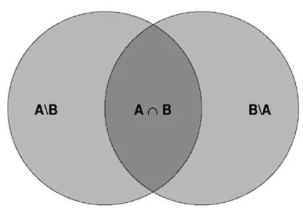
Fig. 1. Venn diagram showing a set-theoretic view of the span of two sets of basis functions (AandB, left and right circles, respectively) in a data space (D) associated with two sets of generic model parameters to be co-estimated in a least-squares sense. Notationally,A∩Bis read “A
intersectionB”,A\Bis read “Aminus the intersection ofAandB”, andB\Ais read “Bminus the intersection ofBandA”.
Indeed, there will be an artificial reduction in power in a predicted target field if contaminating fields are removed in a separate first step. Notice, however, that this says nothing about the relative lengths of the co-estimated and serial estimated parameter state vectors; intuitively, it seems that the latter should somehow have power artificially removed, but evidently it is estimated such that Eq. (8) holds. In fact, an upper-bound on the ratio of the lengths ofx˜B toxB is
found in Appendix 1 to be
x˜B
|xB| ≤
κBTN
AB
, (11)
whereκBTN
AB
is the condition number ofBTN AB, i.e.,
the ratio of the largest to smallest eigenvalues of BTN
AB
(see Demmel, 1997). Since the condition number is always ≥ 1, this does not force a reduction in power in x˜B with
respect to xB. These properites will be illustrated in an
example using theSwarmconstellation in Section 4.1, and in this case it will be seen that actually|xB|<x˜B.
The rationale for using least-squares co-estimation rather than serial estimation may be further illustrated through set-theoretic arguments by considering a data spaceDin which
dand the columns of AandB reside. Let the span of the columns of Aand B be represented by circles; the circles then delineate that part of Dthat may be described by the columns of either Aor B. By construction, there are four distinct regions: that which may be described by bothAand B, that is, the intersection of AandBdenoted A∩B; that which may be described byA, but notB, denotedA\B; that which may be described by B, but not A, denoted B\ A; and that which is described by neither A nor B. This is represented visually in the Venn diagram of Fig. 1.
beforexB in a serial approach, thenxA is fit by the entire
span of A, i.e., the entire circle representing A, followed byxB being fit by the entire span of B. However, A∩ B
in some sense represents “disputed territory” within which the estimator cannot discriminate between the two overlap-ping sets. BecauseA∩Bis not barred from consideration,
xA, being the first parameter set, will remove power from
this region whilexB, finding no power here, will effectively
damp this portion of its data space. Note that a reversal in order will necessarily change the solutions.
By contrast, co-estimation will eliminate A ∩ B from consideration and rather estimatexAfromA\BandxBfrom
B\A, that is, consider only “undisputed territory”, which is logically appealing. The setsA\BandB\Atranslate into NBA andNAB, respectively, while A∩ B translates into
the span of the columns ofRBAandRAB. It is interesting
to note that ifAandBrepresent mutually orthogonal basis functions under a sufficient data distribution, thenA∩B=
and serial and co-estimation will be equivalent.
3.
Methodology
The justification for a CI paradigm was established in the previous section. The details of its application toSwarm will now be covered, including cases where data have been selected from one to four satellites comprising what is known asSwarmconstellation #2 (Olsenet al., 2006). In addition, parameter modifications to the basic CM4 tem-plate and the estimation procedure will be discussed along with computational issues, which were quite formidable.
3.1 Data
The Swarm constellation #2 is actually a pool of six satellite ephemerides of which up to four have been drawn in this study, details of which are provided in Olsenet al. (2006). In the first case, only a single low satellite is used, SwarmA, with initial altitude and inclination of 450 km and 86.8◦, respectively; the second case uses both low-flying satellites, Swarm A and B, differing only in their right-ascension of the ascending node (RAAN), resulting in a longitudinal separation of 1.5◦; the third case adds a single high-flying satellite, Swarm C, to the mix whose initial altitude and inclination are 550 km and 87.3◦, respectively; and finally, the fourth case adds still another high-flyer, SwarmD, with identical initial altitude and inclination as SwarmC, but with a RAAN of 348◦, which separates it by 12◦in longitude fromSwarmC, whose RAAN is 0◦.
Vector magnetic data were synthesized along the ephemerides every 1 min from 1997 to 2002 from a pro-totype of the CM4 model (Sabakaet al., 2004), but with four important modifications: 1) high-degree lithospheric models (up ton =120) and secular variation models (up to n = 20) were added; 2) the magnetospheric field was de-termined hourly from a world-wide distribution of ground-based observatories; 3) a 3-D model of electrical conductiv-ity of the crust and mantle was used to compute the induced signal from the magnetosphere (the induced signal from the ionosphere is still synthesized from a 1-D conductivity model); and 4) realistic magnetic noise from spacecraft and payload was added (Olsenet al., 2006). This synthetic noise is based upon CHAMP spacecraft experience andSwarm specifications. It is a random noise that is correlated in
time, but uncorrelated among the vector components. The standard deviation of the noise is (0.07,0.1,0.07)nT for
(Br,Bθ,Bφ), where(r, θ, φ), are the usual spherical
coordi-nates, in agreement withSwarmperformance requirements. Furthermore, the toroidal field from CM4 was not included in the synthesis because it was found to be somewhat un-realistic, especially at the low satellite altitudes; neither an extrapolation of the Ørsted field in radius nor the Magsat field in local time is stable due to insufficient coverage in the variation of these parameters.
The 1997 to 2002 time span was chosen to mimic that portion of the solar cycle through which the mission is scheduled to fly with the intent of producing magnetic con-ditions similar to those anticipated to be encountered. Two time sampling strategies were used: the first selects 1 min values at quiet-times only during the 1997–2002 mission envelope, wheret is considered quiet when Kp(t) < 1+,
Kp(t−3 hr)≤20,|Dst| ≤20 nT, and|Dst/t| ≤3 nT/hr
(t = 1 hr); the second selects all 1 min values during the 1999–2002 time span, regardless of the magnetic dis-turbance level. The motivation for the first scheme is to test the recoverability of the core SV signal over the entire mission in the case of a realistically restricted data distri-bution; the second scheme facilitates the assessment, in the frequency domain, of the transfer function associated with the 3-D conductivity model, which must be computed at equal increments from the resulting model time-series es-timates of the magnetospheric and high-frequency (periods substantially shorter than those described by SV) induced fields. After 1999 there is either sufficient separation be-tween the high-low satellite orbital planes or they are at least counter-rotating; two conditions which aid in resolv-ing fine-scale structure. In both schemes, the vector data were generated in the local NEC, i.e., (North, East, Center) coordinate system, implying that vector attitude error has not been considered at this stage.
Ground-based observatory data were omitted from the present study mostly to gauge the effectiveness of the con-stellation alone in meeting mission requirements and to simplify this initial investigation. It is expected that sep-arability between the static, broad-scale internal field and the static ionospheric baseline field (Sabakaet al., 2002), used to negate this field on the nightside due to diminished conductivity levels, will be degraded somewhat, but this is not expected to unduly affect target field recovery.
3.2 Parameterization
Since the essence of the CI is the estimation of param-eters associated with an underlying CM, the parameteriza-tion used here follows closely that of CM4, combined of course with modifications which address those found in the forward module listed in the previous section. A brief sum-mary of the model parameterization is now given, but de-tailed descriptions of the portions consistent with CM4 may be found in Sabakaet al.(2002, 2004). The core and litho-spheric magnetic fields are expressed as negative gradients of internal potential functions of the form
Vcl(t,r)=
a
120
n=1
n
m=0
a r
n+1 γm
n (t)Y m n (θ, φ)
with
Ynm(θ, φ)= P m
n (cosθ)expi mφ, (13)
wherea is the mean radius of the Earth (6,371.2 km),ris the position vector, (r,θ,φ) are the usual geographic spher-ical polar coordinates, and Ym
n and Pnm are the Schmidt
quasi-normalized surface spherical harmonic and associ-ated Legendre function of degree n and orderm, respec-tively (Langel, 1987). The {·}operation takes the real part of the expression only. Hence, theγnmare unique complex
expansion coefficients, also known as Gauss coefficients. They are related to the usual real Gauss coefficientsgm
n and
hm
n according toγ m
n =g
m
n −i h
m
n. A degree truncation level
of 120 is used, which is commensurate with the signal con-tent from this source in the data.
As in CM4, cubic B-splines describe the time varia-tions inγ˙m
n (t), and hence, the underlying core SV. In this
study, the epoch is taken at the synthetic mission mid-point, 1999.5, which is also the position of the single interior knot. This configuration is the same for all Gauss coefficients of n ≤20; aboven =20 all coefficients are considered con-stant. This gives a total of 16,840 real parameters describ-ing the core and lithospheric fields.
The ionospheric field is assumed to be due to currents flowing in a sheet at h = 110 km altitude, and so is represented as the negative gradient of potential functions above and below the sheet, across which the radial field is continuous. Since the conductivity pattern governing the current flow is highly organized about the ambient mag-netic field, special harmonic basis functions are employed which possess this symmetry via their dependence upon the Quasi-dipole (QD) coordinate system (Richmond, 1995). Since the currents are ultimately driven by thermal winds due to variable atmospheric heating, these QD functions are mostly sun-synchronous, but include some faster and slower modes to account for main field interactions. Further solar dependence is built in as seasonal fluctuation and a rigid expansion-contraction response to solar radio flux. Al-though the dominant morphology of the quiet, regular (Sq) portion of the ionospheric field is due to the broad-scale, coupled Sq vortices in the northern and southern hemi-spheres, there is a significant signal associated with the nar-row, sinuous equatorial electrojet (EEJ), which is present on the dayside along the dip equator. Therefore, the required QD latitudinal resolution is much higher than in longitudi-nal (or magnetic local time in the sun-synchronous frame).
The induced contributions are assumed due to ana priori four layer, 1-D, radially varying conductivity model derived from Sq and Dst data at selected European observatories
(Olsen, 1998). Responses with seasonal or longer periods are derived by assuming that the mantle is an insulator in the regiona−δ≤r≤aand superconducting inr<a−δ, whereδ=1000 km and corresponds to periods longer than about a week.
This information is quantified in the following parameter-izations inl
kspfor the ionospheric potentials in the regions
a≤r ≤a+h(included for completeness even though sur-face data were not used in this study) andr >a+h, where
the “” indicates the latter region,
Vion(t,tmut,r)=
where the asterisk denotes complex conjugation, (r,θd,φd)
are dipole spherical polar coordinates, t is universal time (UT) in years, tmut is magnetic universal time (MUT) in
hours, whose reference meridian is the prime of the dipole coordinate system, andsandωsare the seasonal
wavenum-ber and fundamental frequency of 1 cycle/yr, respectively, whilepandωpare the diurnal wavenumber and
fundamen-tal frequency of 1 cycle/24 hrs, respectively. Summations overs reflect annual and semi-annual seasonal variability while those over p reflect the first four dominant subhar-monics (periods as short as 6 hrs). Summations overland kare designed to maintain a constant resolution level in QD latitude of about 4◦ for each p value. Thedlm
kn are
coeffi-cients of spherical transforms used in representing the har-monic QD function of degreekand orderl as linear com-binations of the usual spherical harmonics of degreenand ordermin dipole coordinates; thenandmsummations re-flect the required truncations levels. Theglmkn are similar to
dknlm, but they also contain information about the radial
con-tinuity of the ionospheric field across the sheet current. The fknsplm contain information about the QD symmetry of the
internal induced fields, and accordingly, information about the transfer function mappings from ionosphere to induced imposed by the 1-D conductivity model; hence, the depen-dence uponsandp. Theglm
kn and f
lm
knspmatrices allow for a
complete representation of ionospheric primary fields above and below the sheet currents and secondary induced fields in Earth’s outer conducting layers in terms of one set of ionospheric primary potential parameters, of which there are 5,520.
3.2.1 Magnetospheric and high-frequency induced fields
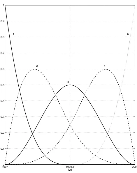
19970 1999.5 2002
Fig. 2. Schematic of the cubic B-spline distribution over the mission envelope used to represent the secular variation of each main field Gauss coefficient. There is a single interior knot at 1999.5 and 4 exterior knots at each endpoint 1997 and 2002. The functions are numbered sequentially from earliest to latest.
unprecedented coverage in local time at a given UT afforded by theSwarmconstellation. It also has the advantage of eliminating the dependence upon theDstindex in tracking
ring current variability, which is known to have shortcom-ings such as baseline shifting, etc. (Olsenet al., 2005), and reducing the dependence ona priori conductivity models. This latter point opens the possibilities of actually deducing information on conductivity structure fromSwarm.
With current sources located outside of the sampling re-gion, these two fields may be represented in the jth bin again as the negative gradient of potentials of the form
Vmag,j(r)=
whereNmaxis the degree truncation level for both field
ex-pansions, andMmxmandMmxiare the order truncation
lev-els for the magnetospheric and induced expansions, respec-tively. The truncation levels of these expansions are influ-enced, as will be seen in Section 4.2, by the bin duration and the configuration of the constellation.
LetT be the bin duration andTa andTb be the
begin-ning and ending times of the mission envelope where the
number of bins is given by=(Tb−Ta)/T and the jth
bin,Bj, is defined asBj ≡[Ta+(j−1)T, Ta+jT)
or B ≡ [Ta+(−1)T,Ta+T]. Comparing
Eqs. (12) and (19), one sees that in function space on T =[Ta,Tb]
constant function onBj. Indexing overkis necessary since
γm
n and ι
k
n,j are with respect to two different coordinate
systems, geographic and dipole, respectively, and spherical harmonics of degreenform an irreducible representation of the rotation group (Cohen-Tannoudjiet al., 1977). Thus, at someT, separation of theιm
n,j fromγ m
n will become
problematic since the former set becomes an increasingly more accurate discretization of the latter with decreasing
T. To remedy the situation, constraints are sought which will enforce some form of orthogonalization between the
ιm
n,j andγnm over the data sampling times, and thus,
tem-porally decorrelate the two fields pointwise in space. Mu-tual adjustment of both sets of parameters in the estima-tion could lead to a highly non-linear optimizaestima-tion prob-lem, and so the high-frequency induced field is made sub-ordinate to the main field. That is, the main field tempo-ral structure is permitted to freely adjust while the induced field is relegated to fit the remaining high-frequency per-turbations superimposed on the former. These perturbation periods would be shorter than the resolving period of the main field basis functions, which are integrals of cubic B-splines, i.e., quartic polynomials within the knot intervals. This is physically reasonable given that there are four poly-nomial roots over 30 months intervals leading to regions of uniform sign on the order of 6 mo in duration inγm
n (t),
which is taken as the resolving period, and this is shorter than variations expected to be seen from core processes due to mantle screening. Thus, theιmn,j are expected to capture
most of the induced field due to the highly variable mag-netospheric field. An obvious caveat is the false attribution of long-period induced signals to the core SV, which are likely manifestations, for instance, of the solar cycle. How-ever, the hope is that real information about the conductivity structure will be gleaned for shorter periods.
Formally, the orthogonality conditions are introduced by defining an inner product, <, >D, on the space of data
sampling times such that for two arbitrary functions f and gdefined onT
to a vector dot product discretized at the data sampling times. In order to enforce orthogonality in time with any main field pointwise in space, the inner product of each set
ιm
n,j, j =1, . . . ,
bi(t) must vanish. In this study, the SV is represented
by cubic B-splines with one interior knot at 1999.5 and 4 exterior knots at each endpoint 1997 and 2002. Each cubic spline occupies 4 adjacent knot intervals giving a total of 5 functions in this case. Figure 2 illustrates the cubic B-spline distribution and numbers the 5 functions sequentially from earliest to latest. For the main field this means 6 basis functions, including a static baseline, at most for any given Gauss coefficient. If the number of real, high-frequency induced coefficients in a bin isLbi = Mmxi(Mmxi+2)+ (Nmax − Mmxi)(2Mmxi +1), then the number of linear,
homogeneous constraints that must be imposed is K = 6Lbi. The form of the constraint corresponding to theith
main field basis function and the induced coefficient of degreenand ordermis
<bi, ιmn >D≡
j=1 ιm
n,j Nj
k=Nj−1+1
bi(tk). (23)
The constraints may be assembled into a matrix equation of the form
Giι=0, (24)
where ι is the vector of all high-frequency induced field expansion coefficients of length Li = Lbi andGi is the
K×Liconstraint matrix. In the equally-incremented
selec-tion scheme, ifNmax=3,Mmxm=1 andMmxi=3 for 1 hr
bins over the three year sampling interval, then=26,304, Lbi =15,Li=394,560,Lbm=9,Lm=236,736
(analo-gous toLbiandLi, respectively, but for the magnetosphere),
and K = 90; thus, a total of Lmi = 631,296 real
coeffi-cients describe the magnetospheric and high-frequency in-duced fields.
3.3 Linear least-squares with linear equality con-straints
The CI employs weighted least-squares to estimate the model parameter state,x, and in this study, incorporates lin-ear equality constraints,Gi, to enforce pointwise temporal
decorrelation between the high-frequency induced field and the core SV field. Because only vector measurements are used, the problem is linear in the model parameters. There-fore, the linear least-squares problem with linear equality constraints (LSLE) may be written as
LSLE
min
x |d−Ax|
2
subject to Gx=0 , (25)
where, d is again the data vector, A is the design matrix associated with x, and G is a sparse matrix whose non-trivial portion corresponds to Gi. Data are weighted
ac-cording to sinθsuch that the resulting distribution is more uniform, which is especially important for polar orbiting satellites. This weighting is understood to have been ap-plied tod and Ain Eq. (25) as a premultiplication by the appropriate√sinθ and will not be discussed further. The solution to LSLE is found directly from the Lagrange multi-plier theorem (Bertsekas, 1995; Golub and Van Loan, 1989; Toutenburg, 1982)
x=
E−1−E−1GTG E−1GT−1G E−1
y, (26)
where
E =ATA, (27)
y=ATd. (28)
It can be seen that the solution in Eq. (26) indeed satisfies the constraint portion of Eq. (25), as required.
Previous CMs derived from POGO, Magsat, Ørsted, and CHAMP satellite data and from observatory data (Sabaka et al., 2002, 2004) have required additional regularization, particularly in the SV and ionospheric portions of the mod-els. This is in part due to inadequacies in data quality and distribution either geographically or in local time. This regularization is usually introduced as additional quadratic smoothing terms (terms whose minima correspond tox = 0) in the least-squares cost function. However, these terms are omitted here in order to investigate whether the quality and distribution ofSwarmdata is satisfactory to resolve all parameters, with the exception of those mentioned earlier. It is expected, however, that reality will be more complicated than this simulation and these regularizations will very well be necessary in selecting the best models.
3.3.1 Computational issues Unless there is a com-pelling need, it is generally not recommended that the sys-tem matrix be explicitely inverted when solving a linear set of equations. Rather, it is more efficient to solve the sys-tem through iterative methods or through matrix factoriza-tion methods such as an “LU” decomposifactoriza-tion. However, Eq. (26) is cast in the form of an explicit matrix inversion since (Sorenson, 1980)
lim λ→∞
E+λGTG−1 =E−1−E−1GT (29)
G E−1GT−1G E−1,
which suggests that a more efficient factorization method may exist.
Consider a partitioning ofxsuch thatxB are the
parame-ters affecting data only in a particularbin, i.e., the magneto-spheric and high-frequency induced parameters, andxC are
the parameters whose effects arecommonto all data, i.e., the core, lithospheric, ionospheric and associated induced parameters. LetGbe that portion ofGcorresponding toxB
such thatG =(G 0). Problem LSLE may alternatively be restated in terms of Lagrange multiplier theory (Bertsekas, 1995; Golub and Van Loan, 1989; Toutenburg, 1982) as
LSLE
min xB,xC
d−AB AC xB
xC
2+ (30)
lim
λ→∞λ|GxB| 2
,
where AB and AC are appropriate partitions of Aandλis
the Lagrange multiplier for the constraint equations. The solution of LSLE is given by the stationary condition
lim λ→∞
EB B+λGTG EBC
ET
BC ECC
xB
xC
=
yB
yC
, (31)
where EB B = ATBAB, EBC = ATBAC, ECC = ATCAC,
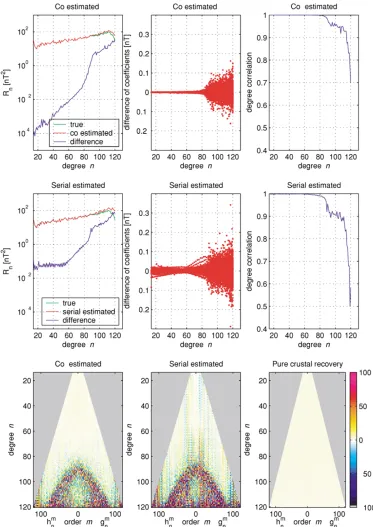
Fig. 3. Comparison of true and recovered crustal field coefficients at Earth’s surface from SW-ABCD data containing both crustal, fromn=14−120, and magnetospheric contributions using both co-estimation and serial estimation schemes. For the top two tiers, the left are theRnspectra for the true (green), recovered (red) and for the difference between true and recovered (blue) crustal models. In the middle are the differences in coefficients as a function of degreen. On the right are the degree correlations,ρn, between the recovered and true models. The bottom tier shows the sensitivity matrices,S(n,m), of the crustal fields recovered by co- (left) and serial (middle) estimation and when the SW-ABCD data contained only a crustal contribution (right).
limλ→∞EB B+λGTG
−1
allows for a relatively straight forward block-Cholesky factorization to be performed se-quentially by bin. This is because theLmi×LmimatrixEB B
has a sparse block-diagonal structure due to the temporally local nature of thexB parameters. There is one symmetric
Lb×Lbblock for each bin, whereLb =Lbi+Lbm. Since
Gmay be easily partitioned across bins, theGE−B B1GT
ma-trix can be easily accumulated sequentially by bin. This is a
great savings over the formation ofG E−1GT sinceE−1 is necessarily dense.
The algorithm then requires one pass through the data for the block-Cholesky factorization phase and a possible sec-ond pass (depending on whether bin-oriented matrices are stored during the first pass) for the back-substitution phase. If Lcli is the length ofxC, which in this study is 22,360,
por-tion of a matrix of order L plus one right-hand-side vec-tor are L(L +3)/2 = 252,574,049 words, where L = Lcli+Lb+K =22,474.
Actual computation was done onhalem, the HP/Compaq AlphaServer Super-Cluster located at the NASA Center for Computational Sciences at Goddard Space Flight Cen-ter. This is a large-scale, distributed-memory, parallel computer. Linear algebraic operations were performed on 64 processors using the ScaLAPACK software as well as theParallel Basic Linear Algebra Subprograms, (PBLAS) and the Basic Linear Algebra Communication Subrou-tines (BLACS). Additional information may be found at http://www.netlib.org/scalapack.
4.
Results and Discussion
In order to assess the quality of recovery of the target fields, three different metrics will be used:
Difference in spectra If gm
n andhmn are the real Gauss
coefficients of the internal field expansion, then the mean-squared field magnitude at Earth’s surface from degreen, Rn, known as the Lowes-Mauersberger spectrum (Langel,
1987), is given by
Rn=(n+1)
wheregn is the vector of spherical harmonic coefficients
of degreen. Hence, Rn is rotationally invariant, and these
spectra, as well as those of the model differences, i.e.,gn,
gauge the agreement in magnitude of the true and recovered
gn.
Degree correlation To gauge the agreement in direction between two vectors, gn,1 andgn,2, of spherical harmonic
coefficients of degreen, the degree correlation,ρn, is
com-puted as
45◦, i.e., the vectors are more correlated than uncorrelated.
Sensitivity matrix To assess the agreement of two mod-els for a particular coefficient, a sensitivity matrix,S(n,m), is constructed in which coefficient differences are normal-ized by the mean spectral amplitude for degreen. If km n
is the recovered Gauss coefficient such thatknm = g m
n is the
correspond-ing true coefficient, then
S(n,m)=100 k
4.1 Recovery using co- versus serial estimation
In Section 2 it was argued that a recovery approach based upon co-estimation of the parameters should be superior to one using serial estimation. In this section, an example is provided which illustrates this in the context ofSwarm where only the magnetospheric and staticn = 14−120 degree lithospheric contributions are taken from the data of the fourSwarmsatellites A, B, C and D, denoted constel-lation SW-ABCD, selected during quiet-time using the cri-teria described earlier. Instrument noise is not considered here. This yields 789,763 vector observations per satel-lite for a total measurement count of dim(d)=9,477,156. These are analyzed over 1 hr bins with magnetospheric ex-pansions defined by Nmax = 3 and Mmxm = 1. This
cor-responds to the hourly analysis of world-wide observatories used to synthesize this data mentioned earlier. In addition, a singleSwarmsatellite traverses roughly 2/3 of an orbit per hour, which should be sufficient for resolving these trunca-tion levels. This results inLbm = Lb =9 coefficients per
1 hr bin. The number of bins having a sufficient amount of data for this parameterization is ≈ 14,000. Thus, the total number of magnetospheric coefficients is about 126,000. If a degreen = 1−120 internal static expan-sion is used to model the lithosphere, then a grand total of dim(x)≈140,640 parameters will be estimated. These pa-rameters are both co-estimated and serial estimated; the lat-ter estimating and removing the magnetospheric contribu-tions from the data first and then estimating the lithospheric field separately. The data weighting is as described in Sec-tion 3.3.
The resulting quality of recovery of the crustal coeffi-cients from these two approaches is illustrated in Fig. 3. The Rn spectra, coefficient differences and degree correlations
all show the degraded nature of the serial recovery with re-spect to co-estimation. This is especially true for the low to mid-degree range where the dispersion of the serial estimate from the true model is over two orders of magnitude higher in Rn than for the co-estimate. It is suspected that this
is the likely range of the parameter space intersection be-tween magnetospheric and lithospheric basis functions. In fact, a test case was attempted in which an additional static n = 1−13 degree lithospheric contribution was retained in the data, but while this was successful for co-estimation, it failed completely for serial estimation, thus embolden-ing the low-degree intersection argument. The most direct comparision is seen in the sensitivity matrices which show spurious excursions in the serial estimate along columns of equal orderm which do not appear in the co-estimate for n<65.
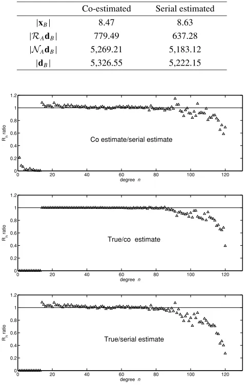
Table 1. Euclidean lengths of crustal parameter state vectors,xB, and various projections of predicted crustal signal vectors,dB, derived from SW-ABCD data containing both crustal, fromn=14−120, and mag-netospheric contributions using both co-estimation and serial estimation schemes. Here,AandBdenote the magnetosphere and crust, respec-tively. Units are in nT.
Co-estimated Serial estimated
|xB| 8.47 8.63
|RAdB| 779.49 637.28
|NAdB| 5,269.21 5,183.12
|dB| 5,326.55 5,222.15
0 20 40 60 80 100 120
0 0.2 0.4 0.6 0.8 1 1.2
degree n Rn
ratio
Co estimate/serial estimate
0 20 40 60 80 100 120
0 0.2 0.4 0.6 0.8 1 1.2
degree n Rn
ratio
True/co estimate
0 20 40 60 80 100 120
0 0.2 0.4 0.6 0.8 1 1.2
degree n Rn
ratio
True/serial estimate
Fig. 4. Ratios of crustalRnvalues at Earth’s surface per degree from the true, co-estimated, and serial estimated models. Top shows co-estimated to serial estimated, middle shows true to co-estimated, and bottom shows true to serial estimated ratios.
parameter state vectors, as derived from co-estimation and serial estimation. Indeed, all of the predicted signal lengths are in accordance with Eq. (8). In addition, the projections onto the range of the magnetospheric column span also show decreased power in the serial estimation case; some-thing intuitively satisfying, but not necessarily required. What is very interesting, however, is that the length of the serial estimate of the crustal parameter vector exceeds that of the co-estimate. Recall from Eq. (11) of Section 2 that the upper-bound on the ratio of the former to the latter is always ≥ 1. Evidently, additional structure is needed in
xB in this case to accommodate the second term in the cost
function of Eq. (7).
In order to investigate this further, plots were made of the ratios of crustalRn values at Earth’s surface per degree
from the true, co-estimated, and serial estimated. While one might consider this a comparison of predicted signals,
the cancellation of then +1 terms in Eq. (33) leaves a simple ratio of parameter variances per degree. The top, middle, and bottom plots in Fig. 4 show the co-estimated to serial estimated, true to co-estimated, and true to serial estimated ratios. Focusing on the n = 14−75 regime reveals an erroneous decrease in parameter strength for the serial estimate, which is not seen in the co-estimate. For n>80, both estimates have excessive power, but even more so for the serial estimate; apparently the high degree terms account for the longer length of the serial estimate. For n < 14, the true model has zero power, but the top plot shows that the serial estimate has significantly more power than the co-estimate.
While this case study shows the superior recovery capa-bility of co-estimation over serial estimation, it does also reveal a problem with the current general analysis which is manifested as a prominent “hemispherical” excursion pat-tern for n > 85 in the sensitivity matrices of both ap-proaches. To investigate this, another test was done in which only the staticn = 14−120 degree lithospheric contribution in the SW-ABCD data was retained. This was analyzed directly using a spherical harmonic expansion of like truncation level in order to see if the pattern was due to some type of sampling inadequacy. The resulting ma-trix at the lower-right of Fig. 3 shows near perfect recov-ery and indicates that no such sampling problem exists. Since the pattern exists even after correction of the crustal basis functions for parameterized magnetospheric effects, as attested to in the co-estimation plot, this suggests that the time-varying magnetospheric field is not being entirely explained by the parameterization used here. If the mag-netosphere were static throughout the mission and mod-elled as such, then one would expect this field to be near-orthogonal, due to possible sampling issues, to the static lithosphere. However, this is a case in which a portion of the unmodelled, time-varying external field appears as a static internal field in the null space of the magnetospheric model; a space shared by both the co-estimation and se-rial estimation. The actual shape, and degree/order range of the excursion pattern is likely related to the orbital in-clination angles of the SW-ABCD satellites. In fact, differ-ence plots between the vector components of the true crustal field and those predicted from co-estimation and serial es-timation (not included here) reveal structure along the or-bits. This type of contamination is common when dealing with data concentrated along tracks and is usually addressed by well-known methods such as levelling (see Green, 1983; Luyendyk, 1997; Minty, 1991), although see the companion paper of Mauset al.(2006) for an alternative approach in crustal field extraction fromSwarm. It is beyond the scope of this paper to pursue the problem any further here and it will be left for future research. However, this will neces-sarily limit the maximum degree of resolution of the crustal field in this study to aboutn=90.
4.2 Recovery from quiet-time data
ex-5 10 15 101
101 103
degree n R n
[(nT/yr)
2 ]
SV at 1997.5
true SW A SW AB SW ABC SW ABCD
0 5 10 15
10 0 10 20 30 40
SV at 1997.5
difference of coefficients [nT/yr]
degree n
5 10 15
0 0.2 0.4 0.6 0.8 1
SV at 1997.5
degree n
degree correlation
5 10 15
101 101 103
degree n R n
[(nT/yr)
2 ]
SV at 1998.5
0 5 10 15
20 15 10 5 0
SV at 1998.5
difference of coefficients [nT/yr]
degree n
5 10 15
0 0.2 0.4 0.6 0.8 1
SV at 1998.5
degree n
degree correlation
5 10 15
101 101 103
degree n R n
[(nT/yr)
2 ]
SV at 1999.5
0 5 10 15
15 10 5 0 5 10 15 20
SV at 1999.5
difference of coefficients [nT/yr]
degree n
5 10 15
0 0.2 0.4 0.6 0.8 1
SV at 1999.5
degree n
degree correlation
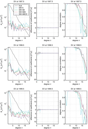
Fig. 5. Comparison of original and recovered secular variation (SV) at 1997.5, 1998.5 and 1999.5 at Earth’s surface for each of the four combinations of satellites, SW-A, SW-AB, SW-ABC, and SW-ABCD. On the left are theRnspectra for the original (black) and for the difference between original and recovered SW-A (light blue), SW-AB (green), SW-ABC (red), and SW-ABCD (dark blue) models. In the middle are the differences in coefficients as a function of degreen(same color scheme). On the right are the degree correlations,ρn, between the recovered and original models (same color scheme).
pansions defined by Nmax = 3 andMmxm = 1. However,
the associated high-frequency induced signal is a function of 3-D conductivity structure and requires a more compli-cated spatial representation. In this case a Nmax = 3 and
Mmxi=3 expansion is used. It will be seen that in order to
resolve these features, one should have satellites in at least two well-separated orbit planes. This results in Lbi = 15
andLbm=9 for a total ofLb =24 coefficients per 1 hr bin.
Recall that the number of bins having a sufficient amount of
data for this parameterization is≈14,000. Thus, the to-tal number of magnetospheric and high-frequency induced coefficients is about 336,000; the grand total of parameters to be estimated is then dim(x)≈358,360. The number of linear orthogonality constraints isK =90.
5 10 15 101
101 103
degree n R n
[(nT/yr)
2 ]
SV at 2000.5
true SW A SW AB SW ABC SW ABCD
0 5 10 15
5 0 5 10 15 20
SV at 2000.5
difference of coefficients [nT/yr]
degree n
5 10 15
0 0.2 0.4 0.6 0.8 1
SV at 2000.5
degree n
degree correlation
5 10 15
101 101 103
degree n R n
[(nT/yr)
2 ]
SV at 2001.5
0 5 10 15
60 40 20 0 20 40
SV at 2001.5
difference of coefficients [nT/yr]
degree n
5 10 15
0 0.2 0.4 0.6 0.8 1
SV at 2001.5
degree n
degree correlation
20 40 60 80
101 101 103
degree n R n
[nT
2 ]
C/L at 1999
20 40 60 80
2 1 0 1 2
C/L at 1999
difference of coefficients [nT]
degree n
20 40 60 80
0 0.2 0.4 0.6 0.8 1
C/L at 1999
degree n
degree correlation
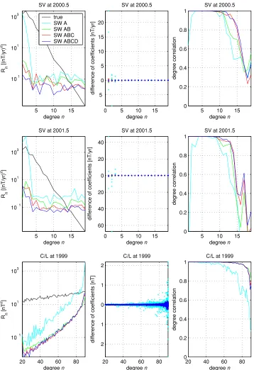
Fig. 6. Same as Fig. 5, but for secular variation (SV) at 2000.5 and 2001.5 and for the core and lithosphere (C/L) at 1999.0 at Earth’s surface (bottom panels).
varies over the life of the mission, being a bit better towards the middle of the mission. Degrees 1–14 are recovered con-sistently above the 0.7 correlation threshold, but degrees up to 16 are recovered at this level during certain times. These values are also confirmed by the cross-over point of the Rn spectra of the original and difference; the degree above
which errors begin to dominate the signal. It is expected that recovery of degrees 1–3 will be enhanced if observa-tory data are used. The sensitivity matrices show a grad-ual degradation across all orders with increasing degree. It should be noted that power associated with any long-term
trends existing in the magnetospheric induced contributions would necessarily be incorporated into that of the SV by de-sign and could be the cause of the observed deteriorations at high degree.
dh
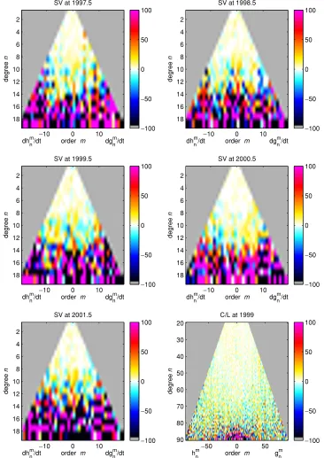
Fig. 7. Sensitivity matrices,S(n,m), for the SW-ABCD secular variation (SV) and core and lithospheric (C/L) models corresponding to the epochs in Fig. 5.
The effects of orbital configuration on the recoverability of the SV and the time-series of magnetospheric and high-frequency induced contributions are illustrated in Figs. 8-11. The first figure shows the main fieldgm
n andhmn
coeffi-cient estimates from SW-ABCD (green) and the original co-efficients (dark blue) over the mission envelope for degrees n=1−3, and the second, third and fourth figures show the same for the SVg˙m
n andh˙mn, the magnetosphericqnmandsnm,
and the high-frequency inducedanmandb m
n coefficients,
re-spectively. Recall that the magnetospheric coefficients are only determined over ordersm =0−1. These real
coeffi-cients are related to the complex such thatγm
n =gnm−i hmn,
μm
n = qnm−i snm andιmn = anm−i bmn. Note that the
ge-ometries are slightly different here since the main field and SV coefficients relate to geographic coordinates while the magnetospheric and induced coefficients relate to dipole co-ordinates. The original magnetospheric and induced coef-ficients have been shifted by various amounts in order to facilitate visual comparisons.
29650
1997 1998 1999 2000 2001 2002 290
1997 1998 1999 2000 2001 2002 700
1997 1998 1999 2000 2001 2002
−500
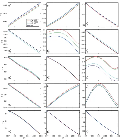
Fig. 8. Plots of the main field coefficientsgm
n =
forn=1−3 over the mission envelope derived from quiet-time data from SW-ABC (red), SW-ABCD (green) and SW-AB (light blue) compared to the true coefficients (dark blue).
for the main field coefficients. However, there are some noteworthy coefficients whose offset mismatches are large with respect to total SV over the mission, e.g, g1
2 andg30.
These offsets could be due to ionospheric baseline leakage due to the absence of surface data, especially since these are low orders. There are also some cases in which simpler con-stellations perform better than SW-ABCD, and these will be discussed later.
Looking at the magnetospheric and high-frequency in-duced coefficients, one notices large oscillations in some of
0 5 10 15 20
dg10/dt
[nT/yr]
SW ABC SW ABCD SW AB true
5 10 15
dg11/dt
−30
−28
−26
−24
−22
−20
dh11/dt
−20
−18
−16
−14
−12
−10
dg20/dt
[nT/yr]
−5 0 5
dg21/dt
−30
−25
−20
−15
−10
dh21/dt
−6
−5
−4
−3
−2
dg22/dt
[nT/yr]
−15
−10
−5
dh22/dt
−2
−1 0 1 2
dg30/dt
−6
−5
−4
−3
−2
dg 3 1
/dt
[nT/yr]
0 2 4 6 8 10
dh 3 1
/dt
−2
−1 0 1 2
dg 3 2
/dt
1997 1998 1999 2000 2001 2002
−5
−4
−3
−2
−1 0
dh32/dt
[nT/yr]
[yr]
1997 1998 1999 2000 2001 2002
−15
−10
−5
dg33/dt
[yr]
1997 1998 1999 2000 2001 2002
−20
−15
−10
−5 0
dh33/dt
[yr]
Fig. 9. Plots of the secular variation coefficientsg˙m
n =
˙ γm
n
andh˙m
n =
˙ γm
n
forn=1−3 over the mission envelope derived from quiet-time data from SW-ABC (red), SW-ABCD (green) and SW-AB (light blue) compared to the true coefficients (dark blue).
high-frequency induced coefficients, to be discussed later, suggests otherwise.
Despite this, excellent recovery is seen in all of the mag-netospheric and most of the high-frequency induced coeffi-cients, particularly during the latter half of the mission and for lower orderm. Table 2 lists the correlations between the true and recovered time-series for the entire mission (1997– 2002) and the latter half of the mission (1999–2002) for each constellations considered in this study. In this context,
1997 1998 1999 2000 2001 2002
1997 1998 1999 2000 2001 2002 −30
1997 1998 1999 2000 2001 2002 −40
1997 1998 1999 2000 2001 2002 −20
1997 1998 1999 2000 2001 2002 −25
1997 1998 1999 2000 2001 2002 −15
1997 1998 1999 2000 2001 2002 −15
1997 1998 1999 2000 2001 2002 −15
1997 1998 1999 2000 2001 2002 −15
Fig. 10. Plots of the magnetospheric coefficientsqmn =
quiet-time data from SW-ABC (red), SW-ABCD (green) and SW-AB (light blue) compared to the true coefficients (dark blue). Vertical dotted lines mark separations of 3, 6, and 9 hr in local time between theSwarmA and C orbital planes; satellites are either co-rotating or counter-rotating for separations less than or greater than 6 hr, respectively. The SW-AB and true coefficients have been shifted in order to facilitate a visual comparison; the shifts forq0
1,q11,. . .,s31are 40, 20, 20, 10, 15, 10, 7, 7 and 7 nT, respectively, for the SW-AB and−40,−20,−25,−10,−15,−10,−7,−7 and −7 nT, respectively, for the true coefficients.
increasingm and do generally increase with larger orbital plane separations seen after 1999. One should realize that while these correlations can be quite modest, they reflect all periods present in the series; it is expected that these val-ues will fluctuate amongst individual periods. In addition,
if the bin duration is increased to allow better spatial cover-age, then these higher-order harmonics are recovered much better, at least below the Nyquist frequency (see Kuvshinov et al., 2006).
−40
1997 1998 1999 2000 2001 2002 −10
1997 1998 1999 2000 2001 2002 −20
1997 1998 1999 2000 2001 2002 −30
Fig. 11. Plots of the high-frequency induced coefficientsamn =
forn= 1−3 over the mission envelope derived from quiet-time data from SW-ABC (red), SW-ABCD (green) and SW-AB (light blue) compared to the true coefficients (dark blue). Vertical dotted lines mark separations of 3, 6, and 9 hr in local time between theSwarmA and C orbital planes; satellites are either co-rotating or counter-rotating for separations less than or greater than 6 hr, respectively. The SW-AB and true coefficients have been shifted in order to facilitate a visual comparison; the shifts fora0
1,a11,. . .,b33are 20, 30, 40, 5, 10, 10, 10, 15, and 15 nT, respectively, for the SW-AB and−20,−30,−40,−5,−10,−10,−3,−3, −10,−10,−15,−5,−5,−10 and−20 nT, respectively, for the true coefficients.
time-series of the recovered high-frequency induced coef-ficients can be seen in Fig. 11 where they all oscillate about the zero level (the true and SW-AB cases have been artifi-cially offset for visual clarity), which is a consequence of being orthogonal to the SV base level; contrast this with the magnetospheric coefficients in Fig. 10 which are not so
Table 2. Correlations between true and recovered magnetospheric (qm
n andsnm) and high-frequency induced (amn andbmn) coefficient time-series derived from constellations SW-ABCD, SW-ABC and SW-AB calculated over the time spans 1997–2002 and 1999–2002.
SW-ABCD
1997–2002 1999–2002
n m am
n q
m
n b
m
n s
m
n a
m
n q
m
n b
m
n s
m n
1 0 0.52089 0.99960 0.50124 0.99981
1 1 0.26071 0.94174 0.28911 0.88463 0.71630 0.99577 0.84385 0.99204
2 0 0.90590 0.99714 0.89910 0.99769
2 1 0.87873 0.99570 0.87833 0.99332 0.83874 0.99750 0.85650 0.99698
2 2 0.45440 — 0.45744 — 0.34466 — 0.40358 —
3 0 0.49713 0.99922 0.59019 0.99948
3 1 0.37767 0.99676 0.35697 0.99215 0.77858 0.99854 0.85185 0.99801
3 2 0.21078 — 0.28762 — 0.43964 — 0.60716 —
3 3 0.04595 — 0.01398 — 0.08002 — 0.11341 —
SW-ABC
1997–2002 1999–2002
n m am
n qmn bnm snm anm qnm bmn snm
1 0 0.48771 0.99908 0.50038 0.99960
1 1 0.22210 0.85373 0.22330 0.72983 0.63666 0.99117 0.68310 0.98354
2 0 0.80750 0.98524 0.83928 0.98852
2 1 0.77784 0.98071 0.75146 0.97199 0.80431 0.99200 0.80241 0.99082
2 2 0.12894 — 0.21288 — 0.09530 — 0.15767 —
3 0 0.41302 0.99764 0.57268 0.99840
3 1 0.22396 0.99250 0.20702 0.98558 0.71814 0.99637 0.77091 0.99539
3 2 0.14945 — 0.17354 — 0.32902 — 0.47520 —
3 3 -0.02989 — 0.00843 — 0.04276 — 0.06703 —
SW-AB
1997–2002 1999–2002
n m am
n q
m
n b
m
n s
m
n a
m
n q
m
n b
m
n s
m n
1 0 0.52190 0.99860 0.48494 0.99841
1 1 0.44273 0.94150 0.40028 0.88620 0.40911 0.94102 0.38576 0.88825
2 0 0.65788 0.96234 0.61189 0.96616
2 1 0.52340 0.92861 0.50112 0.89402 0.42775 0.91093 0.41887 0.88248
2 2 — — — — — — — —
3 0 0.61336 0.98957 0.54623 0.99110
3 1 0.32168 0.90647 0.35988 0.85536 0.30101 0.86682 0.36068 0.83207
3 2 — — — — — — — —
3 3 — — — — — — — —
4.2.2 SwarmA, B and C This case, denoted as SW-ABC, is identical to the previous except that data from Swarmsatellite D, one of the high-flyers, has been removed; thus, dim(d) = 7,107,867. The salient difference is that there is now one less orbital plane during maximum sep-aration, which is expected to somewhat degrade recovery performance. Again, Figs. 5 and 6 indicate that high-degree SV recovery behaves generally the best towards the mid-dle of the mission, where it is commensurate with SW-ABCD, and is only marginally worse than SW-ABCD near the edges. The sensitivity matrices, shown in Fig. 12, are also very close to those of SW-ABCD. Evidently, the
re-moval of SwarmD would not greatly impact the SV re-covery phase of the mission, at least as suggested by these metrics. A closer inspection of individual coefficients for degreesn =1−3 in Figs. 8 and 9 reveals an overall simi-lar behavior in SV with SW-ABCD (green) with perhaps a slight degradation for SW-ABC (red), particularly near the mission edges. Offsets in the main field coefficients are also mostly similar.
SW-dh
Fig. 12. Same as Fig. 7, but for the SW-ABC case.
ABCD, which suggest that for lithospheric studies there is no compelling advantage of SW-ABCD over SW-ABC.
A more noticeable difference in performance between SW-ABCD and SW-ABC is seen in the recovery of the magnetospheric and high-frequency induced time-series, although they are both quite comparable. Figure 10 shows that the SW-ABC (red) recovery of magnetospheric coef-ficients is nearly commensurate with SW-ABCD (green); onlyq11 ands11 exhibit much more oscillation in the
SW-ABC case, and this is only early in the mission. Table 2 supports this numerically and shows very little difference after 1999. Figure 11 shows similar plots for the high-frequency induced coefficients where SW-ABCD (green) and SW-ABC (red) performance is still rather close; of par-ticular exception is thea2
2 andb22pair, which is much more