Principled Selection of Hyperparameters in the Latent Dirichlet
Allocation Model
Clint P. George [email protected]
Informatics Institute University of Florida Gainesville, FL32611, USA
Hani Doss [email protected]
Department of Statistics University of Florida Gainesville, FL32611, USA
Editor:David Blei
Abstract
Latent Dirichlet Allocation (LDA) is a well known topic model that is often used to make inference regarding the properties of collections of text documents. LDA is a hierarchical Bayesian model, and involves a prior distribution on a set of latent topic variables. The prior is indexed by certain hyperparameters, and even though these have a large impact on inference, they are usually chosen either in an ad-hoc manner, or by applying an algorithm whose theoretical basis has not been firmly established. We present a method, based on a combination of Markov chain Monte Carlo and importance sampling, for estimating the maximum likelihood estimate of the hyperparameters. The method may be viewed as a computational scheme for implementation of an empirical Bayes analysis. It comes with theoretical guarantees, and a key feature of our approach is that we provide theoretically-valid error margins for our estimates. Experiments on both synthetic and real data show good performance of our methodology.
Keywords: Empirical Bayes inference, latent Dirichlet allocation, Markov chain Monte Carlo, model selection, topic modelling.
1. Introduction
Latent Dirichlet Allocation (LDA, Blei et al. 2003) is a model that is used to describe high-dimen-sional sparse count data represented by feature counts. Although the model can be applied to many different kinds of data, for example collections of annotated images and social networks, for the sake of concreteness, here we focus on data consisting of a collection of documents. Suppose we have a corpus of documents, say a collection of news articles, and these span several different topics, such as sports, medicine, politics, etc. We imagine that for each word in each document, there is a latent (i.e. unobserved) variable indicating a topic from which that word is drawn. There are several goals, but two principal ones are to recover an interpretable set of topics, and to make inference on the latent topic variables for each document.
To describe the LDA model, we first set up some terminology and notation. There is a vocab-ularyV ofV words; typically, this is taken to be the union of all the words in all the documents of the corpus, after removing stop (i.e. uninformative) words. (Throughout, we use “word” to refer to either an actual word, or to a phrase, such as “heart attack”; LDA has implementations that deal
c
with each of these.) There areDdocuments in the corpus, and ford= 1, . . . , D, documentdhas ndwords,wd1, . . . , wdnd. The order of the words is considered uninformative, and so is neglected. Each word is represented as an index vector of dimension V with a 1 at thesth element, where sdenotes the term selected from the vocabulary. Thus, document dis represented by the matrix
wd= (wd1, . . . , wdnd)and the corpus is represented by the listw = (w1, . . . ,wD). The number
of topics,K, is finite and known. By definition, a topic is a distribution overV, i.e. a point in the simplexSV ={a∈RV :a1, . . . , aV ≥ 0,PVj=1aj = 1}. Ford= 1, . . . , D, for each wordwdi, zdi is an index vector of dimensionK which represents the latent variable that denotes the topic from whichwdi is drawn. The distribution ofzd1, . . . , zdnd will depend on a document-specific
variableθdwhich indicates a distribution on the topics for documentd.
We will useDirL(a1, . . . , aL)to denote the finite-dimensional Dirichlet distribution on the sim-plexSL. Also, we will useMultL(b1, . . . , bL)to denote the multinomial distribution with number of trials equal to1and probability vector (b1, . . . , bL). We will form a K×V matrixβ, whose tth row is thetth topic (howβ is formed will be described shortly). Thus, βwill consist of vec-torsβ1, . . . , βK, all lying inSV. The LDA model is indexed by hyperparametersη ∈ (0,∞)and
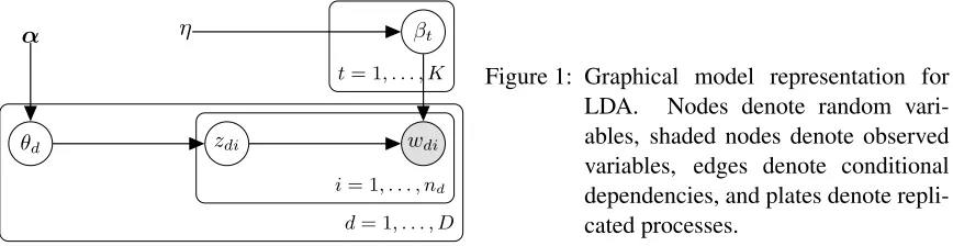
α ∈ (0,∞)K. It is represented graphically in Figure 1, and described formally by the following hierarchical model:
1. βt iid
∼DirV(η, . . . , η), t= 1, . . . , K.
2. θd iid
∼DirK(α), d= 1, . . . , D, and theθd’s are independent of theβt’s.
3. Given θ1, . . . , θD, zdi iid
∼ MultK(θd), i = 1, . . . , nd, d = 1, . . . , D, and the D matrices (z11, . . . , z1n1), . . . ,(zD1, . . . , zDnD)are independent.
4. Givenβand thezdi’s, thewdi’s are independently drawn from the row ofβindicated byzdi, i= 1, . . . , nd, d= 1, . . . , D.
From the description of the model, we see that there is a latent topic variable for every word that appears in the corpus. Thus it is possible that a document spans several topics. Also, because β
is chosen once, at the top of the hierarchy, it is shared among theDdocuments. Thus the model encourages different documents to share the same topics, and moreover, all the documents in the corpus share a single set of topics defined byβ.
wdi
zdi
θd
α η βt
i= 1, . . . , nd
d= 1, . . . , D
t= 1, . . . , K Figure 1: Graphical model representation for
LDA. Nodes denote random vari-ables, shaded nodes denote observed variables, edges denote conditional dependencies, and plates denote repli-cated processes.
Let θ = (θ1, . . . , θD), zd = (zd1, . . . , zdnd) for d = 1, . . . , D, z = (z1, . . . ,zD), and let
ψ = (β,θ,z). The model is indexed by the hyperparameter vectorh= (η,α)∈(0,∞)K+1. For any givenh, lines1–3induce a prior distribution onψ, which we will denote byνh. Line4gives the likelihood. The wordsware observed, and we are interested inνh,w, the posterior distribution
be a symmetric Dirichlet, although arbitrary Dirichlets are sometimes used. Our model allows for arbitrary Dirichlets, for the sake of generality, but in all our examples we use symmetric Dirichlets because a high-dimensional hyperparameter can cause serious problems. We return to this point at the end of Section 2.1.
The hyperparameter vectorh is not random, and must be selected in advance. It has a strong effect on the distribution of the parameters of the model. For example, whenηis large, the topics tend to be probability vectors which spread their mass evenly among many words in the vocabulary, whereas whenη is small, the topics tend to put most of their mass on only a few words. Also, in the special case whereα = (α, . . . , α), so thatDirK(α)is a symmetric Dirichlet indexed by the single parameterα, whenαis large, each document tends to involve many different topics; on the other hand, in the limiting case whereα→0, each document involves a single topic, and this topic is randomly chosen from the set of all topics.
The preceding paragraph is about the effect ofhon the prior distribution of the parameters. We may think about the role ofhon statistical inference by considering posterior distributions. Letgbe a function of the parameterψ. For example,g(ψ)might be the indicator of the eventkθi−θjk ≤, whereiandjare the indices of two particular documents,is some user-specified small number, andk · kdenotes ordinary Euclidean distance in RK. In this case, the value ofg(ψ) gives a way
of determining whether the topics for documentsiandj are nearly the same (g(ψ) = 1), or not (g(ψ) = 0). Of interest then is the posterior probabilityνh,w(kθi −θjk ≤ ), which is given by
the integralR g(ψ)dνh,w(ψ). In another example, the functiongmight be taken to measure the
distance between two topics of interest. In Section 2.4 we demonstrate empirically that the posterior expectation given by the integralR g(ψ)dνh,w(ψ)can vary considerably withh.
To summarize: the hyperparameterhcan have a strong effect not only on the prior distribution of the parameters in the model, but also on their posterior distribution; therefore it is important to choose it carefully. Yet in spite of the very widespread use of LDA, there is no method for choosing the hyperparameter that has a firm theoretical basis. In the literature, h is sometimes selected in some ad-hoc or arbitrary manner. A principled way of selecting it is via maximum likelihood: we letmw(h) denote the marginal likelihood of the data as a function of h, and use
ˆ
h = arg maxhmw(h) which is, by definition, the empirical Bayes choice of h. We will write
m(h) instead of mw(h) unless we need to emphasize the dependence on w. Unfortunately, the
functionm(h)is analytically intractable:m(h)is the likelihood of the data with all latent variables integrated or summed out, and from the hierarchical nature of the model, we see that m(h) is a very large sum, because we are summing over all possible values ofz. Blei et al. (2003) propose estimatingarg maxhm(h)via a combination of the EM algorithm and “variational inference” (VI-EM). Very briefly, w is viewed as “observed data,” andψ is viewed as “missing data.” Because the “complete data likelihood”ph(ψ,w)is available, the EM algorithm is a natural candidate for estimatingarg maxhm(h), sincem(h) is the “incomplete data likelihood.” But the E-step in the algorithm is infeasible because it requires calculating an expectation with respect to the intractable distributionνh,w. Blei et al. (2003) substitute an approximation to this expectation. Unfortunately,
advantages and disadvantages of these two approximations to the EM algorithm are discussed in Section 5.1.
Wallach et al. (2009) give an overview of a class of methods for estimating a combination of some parameter components and some hyperparameter components and, in principle, these pro-cedures could be adapted to the problem of estimating h. The methods they present differ from EM-based approaches in two fundamental respects: (1) they work with an objective function which is not the marginal likelihood functionm(h), but rather a measure of the “predictive performance of the LDA model indexed byh,” and (2) evaluation of their objective function at hyperparameter valuehrequires running a Markov chain, and this has to be done “for each value ofh” before doing the maximization of the objective function, which can impose a heavy computational burden. This paper is discussed further in Section 5.
Another approach for dealing with the problem of having to make a choice of the hyperparame-ter vector is the fully Bayes approach, in which we simply put a prior on the hyperparamehyperparame-ter vector, that is, add one layer to the hierarchical model. For example, we can either put a flat prior on each component of the hyperparameter, or put a gamma prior instead. While this approach can be useful, there are reasons why one may want to avoid it. On the one hand, if we put a flat prior then one problem is that we are effectively skewing the results towards large values of the hyperparameter components. A more serious problem is that the posterior may be improper. In this case, insidi-ously, if we use Gibbs sampling to estimate the posterior, it is possible that all conditionals needed to implement the sampler are proper; but Hobert and Casella (1996) have shown that the Gibbs sampler output may not give a clue that there is a problem. On the other hand, if we use a gamma prior, then at least in the case of a symmetric Dirichlet on theθd’s, we have not made things any easier: we have to specify four gamma hyperparameters. Another reason to avoid the fully Bayes approach is that, in broad terms, the general interest in empirical Bayes methods arises in part from a desire to select a specific value of the hyperparameter vector because this gives a model that is more parsimonious and interpretable. This point is discussed more fully (in a general context) in George and Foster (2000) and Robert (2001, Chapter 7).
In the present paper we show that while it is not possible to computem(h)itself, it is neverthe-less possible, with a single MCMC run, to estimate the entire functionm(h)up to a multiplicative constant. Before proceeding, we note that ifcis a constant, then the information regardinghgiven by the two functionsm(h)andcm(h)is the same: the same value ofhmaximizes both functions, and the second derivative matrices of the logarithm of these two functions are identical. In particu-lar, the Hessians of the logarithm of these two functions at the maximum (i.e. the observed Fisher information) are the same and, therefore, the standard point estimates and confidence regions based onm(h)andcm(h)are identical. Letgbe a function ofψand letI(h) =R g(ψ)dνh,w(ψ)denote
the posterior expectation ofg(ψ). We also show that it is possible to estimate the entire function I(h)with a single MCMC run.
As we will see in Section 2, our approach for estimating m(h) up to a single multiplicative constant andI(h)has two requirements: (i) we need a formula for the ratioνh1(ψ)/νh2(ψ)for any two hyperparameter valuesh1 andh2, and (ii) for any hyperparameter valueh, we need an ergodic Markov chain whose invariant distribution is the posteriorνh,w. This paper is organized as follows.
In Section 3 we consider synthetic data sets generated from a simple model in which h is low dimensional and known, and we show that our method correctly estimates the true value ofh. In Section 4 we describe two Markov chains which satisfy requirement (ii) above. In Section 5 we compare, both theoretically and empirically, the various methods of estimating the maximizer of the marginal likelihood function, in terms of accuracy. Then we compare the various choices of the hyperparameter that are used in the literature—those that are ad-hoc and those that estimate the maximizer of the marginal likelihood function—through a standard criterion that is used to evaluate topic models, and we show that our method performs favorably. In Section 6 we make some concluding remarks, and the Appendix contains some of the technical material that is needed in the paper.
2. Estimation of the Marginal Likelihood up to a Multiplicative Constant and Estimation of Posterior Expectations
This section consists of four parts. In Section 2.1 we show how the marginal likelihood function can be estimated (up to a constant) with a single MCMC run. Section 2.2 concerns estimation of the posterior expectation of a functiong of the parameterψ, given by the integral Rg(ψ)dνh,w(ψ),
and which depends onh. We show how the entire family of posterior expectations{I(h), h ∈ H} can be estimated with a single MCMC run. In Section 2.3 we explain that the simple estimates given in Sections 2.1 and 2.2 can have large variances, and we present estimates which are far more reliable. In Section 2.4 we illustrate our methodology on a corpus created from Wikipedia.
LetH = (0,∞)K+1 be the hyperparameter space. For anyh ∈ H,ν
h andνh,ware prior and
posterior distributions, respectively, of the vectorψ = (β,θ,z), for which some components are continuous and some are discrete. We will use`w(ψ)to denote the likelihood function (which is
given by line4of the LDA model).
2.1 Estimation of the Marginal Likelihood up to a Multiplicative Constant
Note that m(h) is the normalizing constant in the statement “the posterior is proportional to the likelihood times the prior,” i.e.
νh,w(ψ) =
`w(ψ)νh(ψ) m(h) .
Now suppose that we have a method for constructing a Markov chain onψ whose invariant distri-bution isνh,w and which is ergodic. Two Markov chains which satisfy these criteria are discussed
in later in this section. Leth∗ ∈ Hbe fixed but arbitrary, and letψ1,ψ2, . . .be an ergodic Markov chain with invariant distributionνh∗,w. For anyh∈ H, asn→ ∞we have
1 n
n
X
i=1
νh(ψi) νh∗(ψi)
a.s. −−→
Z
νh(ψ) νh∗(ψ)
dνh∗,w(ψ)
= m(h) m(h∗)
Z
`w(ψ)νh(ψ)/m(h)
`w(ψ)νh∗(ψ)/m(h∗)
dνh∗,w(ψ)
= m(h) m(h∗)
Z
νh,w(ψ)
νh∗,w(ψ)
dνh∗,w(ψ)
= m(h) m(h∗)
.
The almost sure convergence statement in (2.1) follows from ergodicity of the chain. (There is a slight abuse of notation in (2.1) in that we have usedνh∗,wto denote a probability measure when we writedνh∗,w, whereas in the integrand,νh,νh∗, andνh∗,wrefer to probability densities.) The signifi-cance of (2.1) is that this result shows that we can estimate the entire family{m(h)/m(h∗), h∈ H}
with a single Markov chain run. Sincem(h∗) is a constant, the remarks made in Section 1 apply,
and we can estimatearg maxhm(h). The usefulness of (2.1) stems from the fact that the average on the left side involvesonly the priors, so we effectively bypass having to deal with the posterior distributions.
The development in (2.1) is not new (although we do not know who first noticed it), and the esti-mate on the left side of (2.1) is not the one we will ultiesti-mately use (cf. Section 2.3); we present (2.1) primarily for motivation. Note that (2.1) is generic, i.e. it is not specific to the LDA model: it is potentially valid for any Bayesian model for which we have a data vectorw, a corresponding like-lihood function`w(ψ), and parameter vectorψ having priorνh, with hyperparameterh ∈ H. We now discuss carefully the scope of its applicability. In order to be able to use (2.1) to obtain valid estimators of the familym(h)/m(h∗), h∈ H, we need the following.
C1 A closed-form expression for the ratio of densitiesνh(ψ)/νh∗(ψ)for some fixedh∗ ∈ H.
C2 A method for generating an ergodic Markov chain with invariant distributionνh∗,w.
We need C1 in order to write down the estimators, and we need C2 for the estimators to be valid.
For notational convenience, let Bn(h) = (1/n)Pn
i=1[νh(ψi)/νh∗(ψi)], and define B(h) = m(h)/m(h∗). In order to use (2.1) to obtain a valid estimator, together with a confidence interval
(confidence set, ifdim(h)>1) forarg maxhm(h), we need in addition the following.
C3 A result that says that the convergence in the first line of (2.1) is uniform inh.
C4 A result that says that ifGn(h)is the centered and scaled version of the estimate on the left side of (2.1) given byGn(h) =n1/2(Bn(h)−B(h)), thenGn(·)converges in distribution to a Gaussian process indexed byh.
We now explain these last two conditions. Generally speaking, for real-valued functionsfn and f defined on H, the pointwise convergence conditionfn(h) → f(h) for each h ∈ Hdoes not imply that arg maxhfn(h) → arg maxhf(h). Indeed, counterexamples are easy to construct, and in Section A.2 of the Appendix we provide a simple one. In order to be able to conclude that arg maxhfn(h) → arg maxhf(h), which is a global condition, we need the convergence of fn to f to be uniform (this is discussed rigorously in Section A.2 of the Appendix). Hence we need C3. Regarding confidence intervals (or sets) for arg maxhf(h), we note thatBn(h) is simply an average, and so under suitable regularity conditions, it satisfies a central limit theorem (CLT). However, we are not interested in a central limit theorem forBn(h), but rather in a CLT for arg maxhBn(h). In this regard, C4 is a “uniform inh CLT” that is necessary to obtain a CLT of the formn1/2(arg maxhBn(h)−arg maxhB(h))
d
We now discuss Conditions C1–C4. Condition C1 is satisfied by the LDA model, and in Sec-tion A.1 of the Appendix we show that the ratio of densitiesνh/νh∗ is given by
νh(ψ) νh∗(ψ)
=
" D
Y
d=1
Γ PK
j=1αj
QK
j=1Γ(αj)
QK
j=1Γ(α∗j) Γ PK
j=1α∗j
K
Y
j=1 θαj−α
∗
j
dj
!#" K
Y
j=1
Γ(V η) Γ(η)V
Γ(η∗)V Γ(V η∗)
V
Y
t=1 βjtη−η∗
#
,
(2.2) whereh∗ = (η∗,α∗).
There are many extensions and variants of the LDA model described in Section 1—too many to even list them all here—and versions of (2.2) can be obtained for these models. This has to be done separately for each case. The features of the LDA model that make it possible to obtain a ratio of densities formula are that it is a hierarchical model, and at every stage the distributions are explicitly finite dimensional. For other models, a ratio of densities formula is obtainable routinely as long as these features exist: when they do, we have a closed-form expression for the prior distribution νh(ψ), and hence a closed-form expression for the ratioνh(ψ)/νh∗(ψ).
Unfortunately, a ratio of densities formula is not always available. A prominent example is the “Hierarchical Dirichlet Processes” model introduced in Teh et al. (2006), which effectively allows infinitely many topics but with finitely many realized in any given document. Very briefly, in this model, for wordiin documentd, there is an unobserved topic ψdi. The latent topic vector
ψd= (ψd1, . . . , ψdnd)has a complicated joint distribution with strength of dependence governed by
a hyperparameterh1(the precision parameter of the Dirichlet process in the middle of the hierarchy), and the D vectors ψ1, . . . ,ψD also have a complicated dependence structure, with strength of dependence governed by a hyperparameter h2 (the precision parameter of the Dirichlet process at the top of the hierarchy). The parameter vector for the model isψ = (ψ1, . . . ,ψD) and the hyperparameter ish= (h1, h2). Unfortunately, the joint (prior) distribution ofψis not available in closed form, and our efforts to obtain a formula forνh(ψ)/νh∗(ψ)have been fruitless.
Regarding Condition C2, we note that Griffiths and Steyvers have developed a “collapsed Gibbs sampler” (CGS) which runs over the vector z. The invariant distribution of the CGS is the con-ditional distribution of z given w. The CGS cannot be used directly, because to apply (2.1) we need a Markov chain on the triple (β,θ,z), whose invariant distribution is νh∗,w. In Section 4 we obtain the conditional distribution of(β,θ)givenzandw, and we show how to sample from this distribution. Therefore, given a Markov chainz(1), . . . ,z(n) generated via the CGS, we can form triples(z(1),β(1),θ(1)), . . . ,(z(n),β(n),θ(n)), and it is easy to see that this sequence forms a Markov chain with invariant distributionνh∗,w. We will refer to this Markov chain as the Aug-mented Collapsed Gibbs Sampler, and use the acronym ACGS. In Section 4 we show that the ACGS is not only geometrically ergodic, but actually is uniformly ergodic. We also show how to sample from the conditional distribution ofzgiven(β,θ)andw. This enables us to construct a two-cycle Gibbs sampler which runs on the pair(z,(β,θ)). We will refer to this chain as the Grouped Gibbs Sampler, and use the acronym GGS. Either the ACGS or the GGS may be used, and we see that Condition C2 is satisfied for the LDA model.
are given in the Appendix. (We have relegated the regularity conditions and a discussion of their significance to the Appendix in order to avoid making the present section too technical.) Letpbe the dimension ofh. Sop= 2if we take the distribution of theθd’s to be a symmetric Dirichlet, and p=K+ 1if we allow this distribution to be an arbitrary Dirichlet.
Theorem 1 Letψ1, ψ2, . . . be generated according to the Augmented Collapsed Gibbs Sampling algorithm described above, letBn(h) be the estimate on the left side of (2.1), and assume that Conditions A1–A6 in Section A.2 of the Appendix hold. Then:
1. arg maxhBn(h)
a.s.
−−→arg maxhm(h).
2. n1/2 arg maxhBn(h)−arg maxhm(h)→ Nd p(0,Σ)for some positive definite matrixΣ.
3. LetΣbnbe the estimate ofΣobtained by the method of batching described in Section A.2 of the
Appendix. Then Σbn a.s.
−−→ Σ, and in particular Σbnis invertible for largen. Consequently, the
ellipseEgiven by
E =h: (arg maxuBn(u)−h)>Σbn−1(arg maxuBn(u)−h)≤χ2p,.95/n
is an asymptotic95%confidence set forarg maxhm(h). Here,χ2p,.95denotes the.95quantile of the chi-square distribution withpdegrees of freedom.
Remark 2 The mathematical development in the proof requires a stipulation (Condition A5) which says that the distinguished point h∗ is not quite arbitrary: if we specify H = [η(L), η(U)]×
[α(L)1 , α(U)1 ]× · · · ×[α(L)K , α(U)K ], thenh∗ must satisfy
η∗ <2η(L) and αj∗ <2α(L)j , j= 1, . . . , K. (2.3)
(Condition(2.3)is replaced by the obvious simpler analogue in the case of symmetric Dirichlets.) Thus, Condition A5 provides guidelines regarding the user-selected value ofh∗.
Remark 3 Part 3 suggests that one should not use arbitrary Dirichlets whenKis large. The ellipse is centered atarg maxuBn(u)and the lengths of its principal axes are governed by the termχ2p,.95. Whenp=K+ 1andKis large,χ2K+1,.95is on the order ofK+ 1, and the confidence set for the empirical Bayes estimate ofhis then huge. In other words, when we use an arbitrary Dirichlet, our estimates are very inaccurate.
Actually, the problem that arises whendim(h) = K is not limited to our Monte Carlo scheme for estimatingarg maxhm(h). There is a fundamental problem, which has to do with the fact that there is not enough information in the corpus to estimate a high-dimensionalh. Suppose we view theDdocuments as being drawn from some idealized population generated according to the LDA model indexed byh0. Leaving aside computational issues, suppose we are able to calculatehˆ = arg maxhm(h), the maximum likelihood estimate ofh0, to infinite accuracy. Standard asymptotics giveD1/2(ˆh−h0)→ Nd p(0,Ω−1)asD→ ∞, whereΩis the Fisher information matrix. Therefore,
2.2 Estimation of the Family of Posterior Expectations
Letg be a function ofψ, and let I(h) = R
g(ψ)dνh,w(ψ) be the posterior expectation ofg(ψ)
when the prior isνh. Suppose that we are interested in estimatingI(h)for allh∈ H. Proceeding as we did for estimation of the family of ratios {m(h)/m(h∗), h ∈ H}, let h∗ ∈ H be fixed
but arbitrary, and letψ1,ψ2, . . .be an ergodic Markov chain with invariant distributionνh∗,w. To
estimateRg(ψ)dνh,w(ψ), the obvious approach is to write
Z
g(ψ)dνh,w(ψ) = Z
g(ψ) νh,w(ψ) νh∗,w(ψ)
dνh∗,w(ψ) (2.4)
and then use the importance sampling estimate(1/n)Pn
i=1g(ψi)[νh,w(ψi)/νh∗,w(ψi)]. This will not work because we do not know the normalizing constants forνh,wandνh∗,w. This difficulty is handled by rewritingR g(ψ)dνh,w(ψ), via (2.4), as
Z
g(ψ) `w(ψ)νh(ψ)/m(h) `w(ψ)νh∗(ψ)/m(h∗)
dνh∗,w(ψ) = m(h∗)
m(h)
Z
g(ψ)νh(ψ) νh∗(ψ)
dνh∗,w(ψ)
= m(h∗)
m(h)
R
g(ψ) νh(ψ)
νh∗(ψ)dνh∗,w(ψ) m(h∗)
m(h)
R νh(ψ)
νh∗(ψ)dνh∗,w(ψ)
(2.5a)
=
R
g(ψ) νh(ψ)
νh∗(ψ)dνh∗,w(ψ)
R νh(ψ)
νh∗(ψ)dνh∗,w(ψ)
, (2.5b)
where in (2.5a) we have used the fact that the integral in the denominator is just1, in order to cancel the unknown constantm(h∗)/m(h)in (2.5b). The idea to expressR g(ψ)dνh,w(ψ)in this way was
proposed in a different context by Hastings (1970). Expression (2.5b) is the ratio of two integrals with respect toνh∗,w, each of which may be estimated from the sequenceψ1,ψ2, . . . ,ψn. We may estimate the numerator and the denominator by
1 n
n
X
i=1
g(ψi)[νh(ψi)/νh∗(ψi)] and
1 n
n
X
i=1
[νh(ψi)/νh∗(ψi)]
respectively. Thus, if we let
w(h)i = Pnνh(ψi)/νh∗(ψi)
e=1[νh(ψe)/νh∗(ψe)] ,
then these are weights, and we see that the desired integral may be estimated by the weighted average
ˆ I(h) =
n
X
i=1
g(ψi)wi(h). (2.6)
2.3 Serial Tempering
Unfortunately, (2.6) suffers a serious defect: unlesshis close toh∗,νhcan be nearly singular with respect toνh∗ over the region where theψi’s are likely to be, resulting in a very unstable estimate. A similar remark applies to the estimate on the left side of (2.1). In other words, there is effectively a “radius” aroundh∗within which one can safely move. To state the problem more explicitly: there
does not exist a singleh∗ for which the ratios νh(ψ)/νh∗(ψ)have small variance simultaneously for allh ∈ H. One way of dealing with this problem is to selectJ fixed pointsh1, . . . , hJ ∈ H that “cover”H in the sense that for every h ∈ H, νh is “close to” at least one of νh1, . . . , νhJ.
We then replaceνh∗ in the denominator by(1/J)
PJ
j=1bjνhj, for some suitable choice of positive
constantsb1, . . . , bJ. Operating intuitively, we say that for anyh∈ H, because there exists at least onejfor whichνhis close toνhj, the variance ofνh(ψ)/[(1/J)
PJ
j=1bjνhj(ψ)]is small; hence the
variance ofνh(ψ)/[(1/J)Pj=1J bjνhj(ψ)]is small simultaneously for allh ∈ H. Whereas for the
estimates (2.1) and (2.6) we need a Markov chain with invariant distribution isνh∗,w, in the present
situation we need a Markov chain whose invariant distribution is the mixture(1/J)PJ
j=1νhj,w.
This approach may be implemented by a methodology called serial tempering (Marinari and Parisi (1992); Geyer and Thompson (1995)), originally developed for the purpose of improving mixing rates of certain Markov chains that are used to simulate physical systems in statistical mechanics. However, it can be used for a very different purpose, namely to increase the range of values over which importance sampling estimates have small variance. We now summarize this methodology, in the present context, and show how it can be used to produce estimates that are stable over a wide range ofh values. Our explanations are detailed, because the material is not trivial and because we wish to deal with estimates of both marginal likelihood and posterior expectations. The reader who is not interested in the detailed explanations can skip the rest of this subsection with no loss regarding understanding the rest of the material in this paper, and simply regard serial tempering as a black box that produces estimates of the marginal likelihood (up to a constant) and of posterior expectations (cf. (2.1) and (2.6)) that are stable over a wideh-region.
To simplify the discussion, suppose that in line2of the LDA model we takeα = (α, . . . , α), i.e.DirK(α)is a symmetric Dirichlet, so thatHis effectively two-dimensional, and suppose that we takeHto be a bounded set of the formH= [ηL, ηU]×[αL, αU]. Our goal is to generate a Markov chain with invariant distribution(1/J)PJ
j=1νhj,w. The updates will sample different components
of this mixture, with jumps from one component to another. We now describe this carefully. Let Ψdenote the state space forψ. Recall thatψ has some continuous components and some discrete components. To proceed rigorously, we will takeνh andνh,wto all be densities with respect to a
measureµon Ψ. DefineL = {1, . . . , J}, and forj ∈ L, suppose thatΦj is a Markov transition function onΨwith invariant distribution equal to the posteriorνhj,w. On occasion we will writeνj
instead ofνhj. This notation is somewhat inconsistent, but we use it in order to avoid having double
and triple subscripts. We haveνh,w=`wνh/m(h)andνhj,w=`wνj/m(hj), j= 1, . . . , J.
Serial tempering involves considering the state spaceL ×Ψ, and forming the family of distri-butions{Pζ, ζ ∈RJ}onL ×Ψwith densities
pζ(j,ψ)∝`w(ψ)νj(ψ)/ζj. (2.7)
dis-tribution equal to (2.7). If we takeζj =am(hj)forj = 1, . . . , J, whereais an arbitrary constant, then theψ-marginal ofpζ is exactly(1/J)PJj=1νhj,w, so we can generate a Markov chain with
the desired invariant distribution. Unfortunately, the valuesm(h1), . . . , m(hJ) are unknown (our objective is precisely to estimate them). It will turn out that for any value ofζ, a Markov chain with invariant distribution (2.7) enables us to estimate the vector(m(h1), . . . , m(hj))up to a constant, and the closerζ is to a constant multiple of(m(h1), . . . , m(hj)), the better is our estimate. This gives rise to a natural iterative procedure for estimating (m(h1), . . . , m(hj)). We now give the details.
LetΓ(j,·)be a Markov transition function onL. In our context, we would typically takeΓ(j,·) to be the uniform distribution onNj, whereNj is a set consisting of the indices of thehl’s which are close tohj. Serial tempering is a Markov chain onL ×Ψwhich can be viewed as a two-block Metropolis-Hastings (i.e. Metropolis-within-Gibbs) algorithm, and is run as follows. Suppose that the current state of the chain is(Li−1,ψi−1).
• A new valuej ∼Γ(Li−1,·)is proposed. We setLi =jwith the Metropolis probability
ρ= min
1,Γ(j, Li−1) Γ(Li−1, j)
νj(ψi−1)/ζj νLi−1(ψi−1)/ζLi−1
, (2.8)
and with the remaining probability we setLi =Li−1.
• Generateψi ∼ΦLi(ψi−1,·).
By standard arguments, the density (2.7) is an invariant density for the serial tempering chain. A key observation is that theψ-marginal density ofpζis
fζ(ψ) = (1/cζ) J
X
j=1
`w(ψ)νj(ψ)/ζj, where cζ = J
X
j=1
m(hj)/ζj. (2.9)
Suppose that(L1,ψ1),(L2,ψ2), . . .is a serial tempering chain. To estimatem(h), consider
c
Mζ(h) = 1 n
n
X
i=1
νh(ψi) (1/J)PJ
j=1νj(ψi)/ζj
. (2.10)
Note that this estimate depends only on theψ-part of the chain. Assuming that we have established that the chain is ergodic, we have
c
Mζ(h)−a.s.−→
Z
νh(ψ)
(1/J)PJ
j=1νj(ψ)/ζj
PJ
j=1`w(ψ)νj(ψ)/ζj cζ
dµ(ψ)
=
Z `
w(ψ)νh(ψ) cζ/J dµ(ψ)
= m(h) cζ/J
.
(2.11)
This means that for any ζ, the family Mζc(h), h ∈ H can be used to estimate the family
To estimate the family of integralsR g(ψ)dνh,w(ψ), h∈ H , we proceed as follows. Let
b
Uζ(h) = 1 n
n
X
i=1
g(ψi)νh(ψi) (1/J)PJ
j=1νj(ψi)/ζj
. (2.12)
By ergodicity we have
b
Uζ(h) a.s. −−→
Z g(ψ)ν
h(ψ) (1/J)PJ
j=1νj(ψ)/ζj
PJ
j=1`w(ψ)νj(ψ)/ζj cζ dµ(ψ)
=
Z `
w(ψ)g(ψ)νh(ψ) cζ/J
dµ(ψ)
= m(h) cζ/J
Z
g(ψ)dνh,w(ψ).
(2.13)
Combining the convergence statements (2.13) and (2.11), we see that
ˆ
Iζst(h) := Ubζ(h)
c
Mζ(h) a.s. −−→
Z
g(ψ)dνh,w(ψ). (2.14)
Suppose that for some constanta, we have
(ζ1, . . . , ζJ) =a(m(h1), . . . , m(hJ)). (2.15)
Thencζ = J/a, and as noted earlier, fζ(ψ) = (1/J)PJ
j=1νhj,w(ψ), i.e. the ψ-marginal of pζ
(see (2.9)) gives equal weight to each of the component distributions in the mixture. (Express-ing this slightly differently, if (2.15) is true, then the invariant density (2.7) becomespζ(j,ψ) = (1/J)νhj,w(ψ), so theL-marginal distribution ofpζ gives mass(1/J)to each point inL.)
There-fore, for large n, the proportions of time spent in the J components of the mixture are about the same, a feature which is essential if serial tempering is to work well. In practice, we can-not arrange for (2.15) to be true, because m(h1), . . . , m(hJ) are unknown. However, the vector (m(h1), . . . , m(hJ))may be estimated (up to a multiplicative constant) iteratively as follows. If the current value isζ(t), then set
ζ1(t+1), . . . , ζJ(t+1)= Mcζ(t)(h1), . . . ,Mcζ(t)(hJ)
. (2.16)
From the convergence result (2.11), we getMcζ(t)(hj) a.s.
−−→ m(hj)/aζ(t), whereaζ(t) is a constant, i.e. (2.15) is nearly satisfied by ζ1(t+1), . . . , ζJ(t+1). To determine the number of iterations needed, at each iteration we record the proportions of time spent in theJ different components of the mix-ture, i.e. the vector (1/n)Pn
i=1I(Li = 1), . . . ,(1/n)Pni=1I(Li=J)
, and we stop the iteration when this vector is nearly uniform. In all our examples, three or four iterations were sufficient. Pseudocode is given in Algorithm 1.
Algorithm 1:Serial tempering. See the discussion in Sec. 2.3 and Appendices A.1 and 4. Data: Observed wordsw
Result: A Markov chain onL ×Ψ
1 specifyh1, . . . , hJ ∈ H; 2 initializeζ1(1), . . . , ζJ(1);
3 initializeψ0 = (β(0),θ(0),z(0)),L0;
4 compute count statisticsndk andmdkv, ford= 1, . . . , D, k= 1, . . . , K, v = 1, . . . , V;
5 fortuning iterationt= 1, . . .do
6 forMCMC iterationi= 1, . . .do
// The Metropolis-Hastings update
// Set Li via the probability ρ given by (2.8)
7 propose indexj∼Γ(Li−1,·);
8 sampleU ∼Uniform(0,1); 9 ifU < ρthen
10 setLi =j;
11 else
12 setLi =Li−1;
// Generate ψi = (β(i),θ(i),z(i))∼ΦLi(ψi−1,·)
13 fordocumentd= 1, . . . , Ddo 14 forwordwdr,r = 1, . . . , nddo
15 sample topic indexz(i)dr via the CGS (Griffiths and Steyvers, 2004); 16 update count statisticsndkandmdkvaccording tozdr(i)andwdr;
17 fortopick= 1, . . . , K do 18 sample topicβk(i)via (4.5); 19 fordocumentd= 1, . . . , Ddo
20 sample the distribution on topicsθ(i)d via (4.5);
// Update tuning parameters ζ1, . . . , ζJ
21 compute the estimatesMcζ(t)(h1), . . . ,Mcζ(t)(hJ)via (2.10) usingψiandζ
(t) 1 , . . . , ζ
(t) J ;
22 set ζ1(t+1), . . . , ζJ(t+1)= Mcζ(t)(h1), . . . ,Mcζ(t)(hJ)
;
c
Mζ(h) defined in (2.10), and to estimate the family of posterior expectations we use Iˆζst(h) =
b
Uζ(h)
c
Mζ(h)(see (2.12) and (2.10)).
We point out that it is possible to estimate the family of marginal likelihoods (up to a constant) by
f
Mζ(h) = 1 n
n
X
i=1
νh(ψi) νLi(ψi)/ζLi
Note that Mfζ(h) uses the sequence of pairs (L1,ψ1),(L2,ψ2), . . ., and not just the sequence
ψ1,ψ2, . . .. To see why (2.17) is a valid estimator, observe that by ergodicity we have
f
Mζ(h) a.s. −−→
Z Z
νh(ψ) νL(ψ)/ζL
·
1 cζ
`w(ψ)νL(ψ)/ζL
dµ(ψ)dσ(L)
=
Z Z
m(h) cζ
νh,w(ψ)dµ(ψ)dσ(L)
=Jm(h) cζ .
(2.18)
(Note that the limit in (2.18) is the same as the limit in (2.11).) Similarly, we may estimate the integralRg(ψ)dνh,w(ψ)by the ratio
˜ Iζst(h) =
n
X
i=1
g(ψi)νh(ψi) νLi(ψi)/ζLi
n
X
i=1
νh(ψi) νLi(ψi)/ζLi
.
The estimateI˜ζst(h) is also based on the pairs (L1,ψ1),(L2,ψ2), . . ., and it is easy to show that ˜
Iζst(h)−a.s.−→R
g(ψ)dνh,w(ψ).
The estimates Mfζ(h)andI˜ζst(h) are the ones that are used by Marinari and Parisi (1992) and
Geyer and Thompson (1995), butMcζ(h)andIˆζst(h)appear to significantly outperformMfζ(h)and
˜ Ist
ζ(h)in terms of accuracy. We demonstrate this in Section 2.4.
Remark 4 Theorem 1 continues to be true when we use the serial tempering chain, as opposed to the simple ACGS. The needed changes are that in the statement of the theoremBnis replaced with
c
Mζ, and Condition A5 is replaced by the following. If h(1), . . . , h(J) are the grid points used in
running the serial tempering chain, then the stipulation onh∗given by(2.3)is satisfied byh(j)for at least one indexj. See the proof of Theorem 1 in the Appendix.
Globally-Valid Confidence Bands for{I(h), h∈ H}Based on Serial Tempering Here we explain how to form confidence bands for the family{I(h), h ∈ H}based on{Iˆζst(h), h ∈ H}. Our arguments are informal, and we focus primarily on the algorithm for constructing the bands. The proof that the method works is given in Section A.3 of the Appendix. We will writeIˆinstead ofIˆζstto lighten the notation. Suppose thatsuph∈Hn1/2|Iˆ(h)−I(h)|has a limiting distribution as
n→ ∞(in the Appendix we explain why such a result is true), and suppose that we know the.95 quantile of this distribution, i.e. we know the valuec.95such that
P
sup h∈H
n1/2|Iˆ(h)−I(h)| ≤c.95
=.95. (2.19)
In this case we may rewrite (2.19) as
P
ˆ
I(h)−c.95/n1/2 ≤I(h)≤Iˆ(h) +c.95/n1/2for allh∈ H=.95,
I(h) ≤U(h)
=.95for eachh ∈ H, and we cannot make any statement regarding simultaneous coverage.)
The difficulty is in obtainingc.95, and we now show how this quantity can be estimated through the method of batching, which is described as follows. The sequenceψ1, . . . ,ψnis broken up into J consecutive pieces of equal lengths called batches. Forj= 1, . . . , J, letIˆj(h)be the estimate of I(h)produced by batchj. Now theIˆj(h)’s are each formed from a sample of sizen/J. Informally, if n is large and n/J is also large, then for j = 1, . . . , J, suph∈H(n/J)1/2|Ijˆ(h)−I(h)|and
suph∈Hn1/2|Iˆ(h)−I(h)|have approximately the same distribution. Therefore, to estimate c.95, we letSj = suph∈H(n/J)1/2|Iˆj(h)−I(h)|, and as our estimate ofc.95we use the95thpercentile of the sequenceS1, . . . , SJ. Unfortunately, the Sj’s are not available, because they involveI(h), which is unknown. So instead we use Sj = suph∈H(n/J)1/2|Iˆj(h)−Iˆ(h)|, in which we have substitutedIˆ(h)forI(h). To conclude, letS[1] ≤ S[2] ≤ · · · ≤ S[J]denote the ordered values of the sequenceS1, . . . ,SJ. We estimatec.95viaS[.95J], and our95%globally-valid confidence band for{I(h), h∈ H}isˆ
I(h)± S[.95J]/n1/2, h∈ H . In the Appendix we show that the probability that the entire function{I(h), h ∈ H}lies inside the band converges to.95asn→ ∞. There are conditions onJ: we need thatJ → ∞andn/J → ∞; a good choice isJ =n1/2. The Markov chain lengthnshould be chosen such that the band is acceptably narrow.
Iterative Scheme for Choosing the Grid The performance of serial tempering depends crucially on the choice of grid pointsh1, . . . , hJ, and it is essential thatarg maxhm(h)be close to at least one of the grid points, for the reason discussed at the beginning of this section. This creates a circular problem: the ideal grid is one that is centered or nearly centered at arg maxhm(h), but arg maxhm(h)is unknown. The problem is compounded by the fact that the grid has to be “tight,” i.e. the pointsh1, . . . , hJ need to be close together. This is because when the corpus is large, ifhj andhj0 are not close, then forj 6=j0,νh
j andνhj0 are nearly singular (each is a product of a large
number of terms—see (2.2)). In the serial tempering chain, this near singularity causes the proposal j ∼ Γ(Li−1,·)(see (2.8)) to have high probability of being rejected, and the chain does not mix
well. To deal with this problem, we use an iterative scheme which proceeds as follows. We initialize the experiment with a fixedh(0) (for exampleh(0) = (1,1)) and a subgrid that “covers”h(0)(for example a subgrid with convex hull equal to[1/2,2]×[1/2,2]). We then subsample a small set of documents from the corpus and run the serial tempering chain to find the estimate of the maximizer of the marginal likelihood for the subsampled corpus, using the current grid setting. We iterate: at iterationt, we seth(t)to be the estimate of the maximizer obtained from the previous iteration, and select a subgrid that coversh(t). As the iteration numbertincreases, the grid is made more narrow, and the number of subsampled documents is increased. This scheme works because in the early iterations the number of documents is small, so the near-singularity problem does not arise, and we can use a wide grid. In our experience, decreasing the dimensions of theα- andη-grids by10% and increasing the number of subsampled documents by10%at each iteration works well. It is very interesting to note that convergence may occur before the subsample size is equal to the number of documents in the corpus, in which case there is no need to ever deal with the entire corpus, and in fact this is typically what happens, unless the corpus is small. (By “convergence” we mean that h(t)is nearly the same as the values from the previous iterations.) Of course, for small corpora the near-singularity problem does not arise, and the iterative scheme can be skipped entirely.
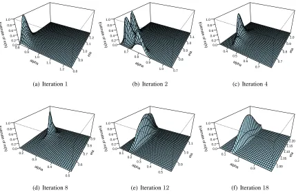
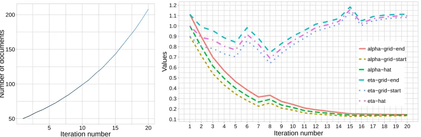
Markov chains of lengthn= 50,000and grids of sizeJ = 100. As will be clear shortly, our results would have been identical ifDhad beenanynumber bigger than105. Figure 2 shows the marginal likelihood surfaces as the iterations progress. At iteration 1, theα-value of the maximizer is outside the convex hull of the grid, and at the second iteration, the grid is centered at that point. Figure 3 gives precise information on the number of subsampled documents (left panel), and the lower and upper endpoints of theα- andη-values used in the grids, as the iterations progress (right panel). The right panel also givesα- andη-values of the estimate of the argmax as the iterations progress. As can be seen from Figure 3, the scheme has effectively converged after about18iterations, and at convergence the number of subsampled documents is only200.
alpha 0.8 0.9 1.0 1.1 1.2 eta 0.8 0.9 1.0 1.1 1.2 Estimate of m(h)
0.0 0.2 0.4 0.6 0.8 1.0
(a) Iteration1
alpha 0.7 0.8 0.9 1.0 eta 0.7 0.8 0.9 1.0 1.1 Estimate of m(h)
0.0 0.2 0.4 0.6 0.8 1.0
(b) Iteration2
alpha 0.4 0.5 0.6 0.7 eta 0.7 0.8 0.9 1.0 Estimate of m(h)
0.0 0.2 0.4 0.6 0.8 1.0
(c) Iteration4
alpha 0.2 0.3 0.4 0.5 eta 0.6 0.7 0.8 0.9 Estimate of m(h)
0.0 0.2 0.4 0.6 0.8 1.0
(d) Iteration8
alpha 0.1 0.2 0.3 0.4 0.5 eta 0.9 1.0 1.1 Estimate of m(h)
0.0 0.2 0.4 0.6 0.8 1.0
(e) Iteration12
alpha 0.1 0.2 0.3 eta 1.00 1.05 1.10 1.15 1.20 Estimate of m(h)
0.0 0.2 0.4 0.6 0.8 1.0
(f) Iteration18
Figure 2: Values ofMc(h)for iterations1,2,4,8,12,18using a synthetic corpus generated
accord-ing to the LDA model withK = 20,nd= 100for eachd,V = 100, andhtrue= (.8, .2).
Serial tempering is a method for enhancing the simple estimator (2.1) which works well when dim(h) is low. The method does not scale well whendim(h)increases. In Section 6 we discuss this issue and present an idea on a different way to enhance (2.1) whenhis high dimensional.
2.4 Illustration on a Wikipedia Corpus
50 100 150 200
5 10 15 20
Iteration number
Number of documents
(a) Number of documents
0.1 0.2 0.3 0.4 0.5 0.6 0.7 0.8 0.9 1.0 1.1 1.2
1 2 3 4 5 6 7 8 9 10 11 12 13 14 15 16 17 18 19 20
Iteration number
V
alues
alpha−grid−end
alpha−grid−start
alpha−hat
eta−grid−end
eta−grid−start
eta−hat
(b) Grid configurations andα- andη-values of estimate of the argmax
Figure 3: Iterations in the serial tempering scheme used on the synthetic corpus in Figure 2: left panel gives the number of documents subsampled at each iteration; right panel gives the specifications for the grid at each iteration.
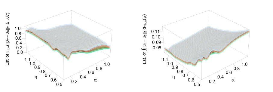
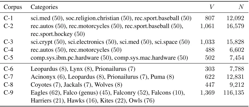
is typically tagged to one or more categories, one of which is the “primary category.” The corpus consists of8documents from the categoryLeopardus,8from the categoryLynx, and7from Prion-ailurus. There are303words in the vocabulary, and the total number of words in the corpus is7788. We tookK = 3, so implicitly we envisage a topic being induced by each of the three categories. The corpus is quite small, but it is challenging to analyze because the topics are very close to each other, so in the posterior distribution there is a great deal of uncertainty regarding the latent topic indicator variables, and this is why we chose this data set. (In our analysis of this corpus, we treat the articles as unlabeled, i.e. we act as if for each article we don’t know the category from which the article is taken.) As mentioned in Section 1, two quantities of interest are the posterior proba-bility that the topic indicator variables for documentsiandj are close, i.e.νh,w(kθi−θjk ≤ ), and the posterior expectation of the distance between topicsiandj, which is given by the integral
R
kβi−βjkdνh,w(ψ). Figure 4 gives plots of estimates of these posterior probabilities and
expec-tations, ashvaries, together with 95%globally-valid confidence sets. The plots clearly show that these posterior probabilities and expectations vary considerably withh.
Each plot was constructed from a serial tempering chain, using the methodology described in Section 2.3. Details regarding the chain and the plots are as follows. We took the sequence h1, . . . , hJ to consist of an 11 ×20 grid of 220 evenly-spaced values over the region (η, α) ∈ [.6,1.1]×[.15,1.1]. For each hyperparameter valuehj (j = 1, . . . ,220), we tookΦj to be the Markov transition function of the Augmented Collapsed Gibbs Sampler alluded to earlier and de-scribed in detail in Section 4 (in all our experiments we used the Augmented Collapsed Gibbs Sampler, but the Grouped Gibbs Sampler gives results which are very similar). We took the Markov transition functionK(j,·)onL ={1, . . . ,220}to be the uniform distribution onNj whereNj is the subset ofLconsisting of the indices of thehl’s that are neighbors of the pointhj. (An interior point has eight neighbors, an edge point has five, and a corner point has three.)1
0.2 0.4 0.60.8
1.0
0.5 0.6 0.7 0.8 0.9 1.0 1.1 0.0 0.2 0.4 0.6 0.8 1.0
a h
Est. of
nh,w
(||
q7
-q8 ||2
£
.07)
0.2 0.4
0.60.8
1.0
0.5 0.6 0.7 0.8 0.9 1.0 1.1 0.08 0.09 0.10 0.11
a h
Est. of
ó õ||b
1
-b2
||2
d
nh,w
(
y
)
Figure 4: Variability of posterior probabilities and expectations for the Cats corpus from Wikipedia. Left panel: estimate of the posterior probability that documents7and8have essentially the same topics, in the sense thatkθ7−θ8k ≤.07, ashvaries. Right panel: estimate of the posterior expectation of the (Euclidean, i.e.L2) distance between topics1and2ash varies.
In Section 2.3, we stated thatMcζ(h)andIˆζst(h)appear to significantly outperformMfζ(h)and
˜ Ist
ζ(h) in terms of accuracy. We now provide some evidence for this, and we will deal with the estimates ofI(h)(a comparison ofMζc(h)andMζf(h)is given in George (2015)). We considered the
Wikipedia Cats corpus described above, and we tookI(h) =νh,w(kθ7−θ8k ≤.07). We calculated ˆ
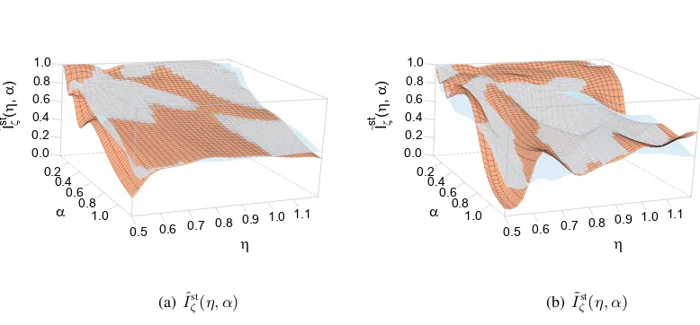
Iζst(h)twice, using two different seeds, and also calculatedI˜ζst(h)twice, using two different seeds, in every case using the sameh-range that was used in Figure 4. The four surfaces were constructed via four independent serial tempering experiments, each involving two iterations (each of length 50,000after a short burn-in period) to form the tuning parameterζ, which was given initial value ζ(0) = ζ1(0), . . . , ζ220(0)= (1, . . . ,1), and one final iteration (of length100,000) to form the estimate ofI(h). Figure 5(a) shows the two estimatesIˆst
ζ(h), and Figure 5(b) shows the two estimatesI˜ζst(h). The figures show that the two independent estimatesIˆζst(h)are close to each other, whereas the two independent estimatesI˜ζst(h)are not.
Although the variability ofIˆst
ζ(h)is significantly smaller than that ofI˜ζst(h), the figures perhaps don’t show this very clearly because a visual comparison of two surfaces is not easy. Therefore, we extracted two one-dimensional slices from each panel in Figure 5, which we used to create Figure 6. The figure shows the values of the two versions ofIˆst
ζ(η, α)and the two versions ofI˜ζst(η, α)when ηis fixed at.70(two left panels); and it shows these plots whenηis fixed at1.00(two right panels). The superiority of Iˆζst overI˜ζst is striking. We mention that, ostensibly, Mcζ(h)andIˆζst(h) require
more computation, but the quantities(1/J)PJ
0.2 0.4
0.6 0.8
1.0
0.5 0.6 0.7 0.8 0.9 1.0 1.1 0.0
0.2 0.4 0.6 0.8 1.0
a
h
Iz
st (h
,
a
)
(a)Iˆζst(η, α)
0.2 0.4
0.6 0.8
1.0
0.5 0.6 0.7 0.8 0.9 1.0 1.1 0.0
0.2 0.4 0.6 0.8 1.0
a
h
Iz
st (h
,
a
)
(b)I˜ζst(η, α)
Figure 5: Comparison of the variability ofIˆζstandI˜ζst. Left panel shows two independent estimates ofI(η, α) =νh,w(kθ7−θ8k ≤.07)usingIˆζst(η, α). Right panel usesI˜ζstinstead ofIˆζst.
3. Empirical Assessment of the Estimator of the Argmax
Consider the LDA model with a given hyperparameter value, which we will denote byhtrue, and suppose we carry out steps 1–4 of the model, where in the final step we generate the corpus w. The maximum likelihood estimate ofh isˆh = arg maxhm(h)and, as we mentioned earlier, for any constant a, known or unknown, arg maxhm(h) = arg maxham(h). As noted earlier, the family
c
Mζ(h), h ∈ H , where Mcζ(h) is given by (2.10), may be used to estimate the family
{m(h), h∈ H}up to a multiplicative constant. So we may usearg maxhMζc(h)to estimateh.ˆ
Recall thatBn(h)is the estimate ofm(h)/m(h∗) given by the left side of equation (2.1). In
theory, arg maxhBn(h) can also be used. However, as we pointed out earlier, Bn(h) is stable only forhclose toh∗—a similar remark applies toIˆ(h)—and unless the region of hyperparameter
values of interest is small, we would not useBn(h)andIˆ(h), and we would use estimates based on serial tempering instead. We have included the derivations of Bn(h) andIˆ(h) primarily for motivation, as these makes it easier to understand the development of the serial tempering estimates. In Section 2.4 we presented an experiment which strongly suggested that Iˆζst(h) is significantly better thanI˜ζst(h)in terms of variance. George (2015) gives experimental evidence that, analogously,
c
Mζ(h)is significantly better thanMfζ(h). Therefore, for the rest of this paper, we use onlyMcζ(h)
andIˆζst(h).
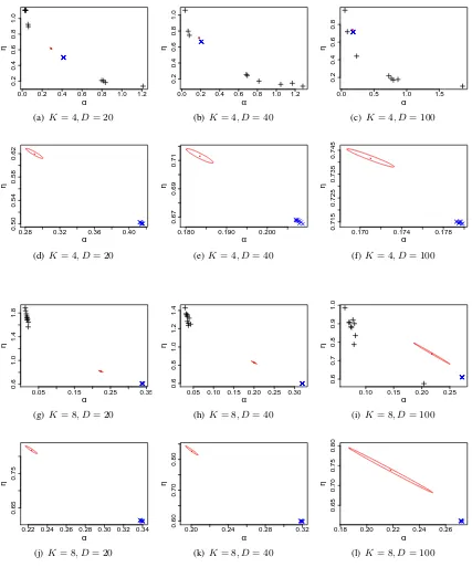
Here we present the results of some experiments which demonstrate good performance ofˆˆh:= arg maxhMcζ(h) as an estimate ofhtrue. We tookα = (α, . . . , α), i.e.DirK(α) is a symmetric
0.2 0.4 0.6 0.8 1.0 1.2
0.0
0.2
0.4
0.6
0.8
1.0
α
I(
h
)
(a)Iˆζst(.70, α)
0.2 0.4 0.6 0.8 1.0 1.2
0.0
0.2
0.4
0.6
0.8
1.0
α
I(
h
)
(b)Iˆζst(1.0, α)
0.2 0.4 0.6 0.8 1.0 1.2
0.0
0.2
0.4
0.6
0.8
1.0
α
I(
h
)
(c)I˜st
ζ(.70, α)
0.2 0.4 0.6 0.8 1.0 1.2
0.0
0.2
0.4
0.6
0.8
1.0
α
I(
h
)
(d)I˜st
ζ(1.0, α)
Figure 6: Two one-dimensional views of the plots in Figure 5. Each of the top two panels shows two independent estimates ofI(η, α), using Iˆζst(η, α). For the left panel,η = 0.70, and for the right panel, η = 1.00. The bottom two panels useI˜ζst instead ofIˆζst. The plots show that the variability ofIˆζstis much smaller than that ofI˜ζst.
evenly-spaced50×50 grid of2500values usingMcζ(h)calculated from a serial tempering chain
implemented as follows. The size of the subgrid was taken to be11×11 = 121, and we used ten iterations of the iterative scheme described in Section 2.3 to form the final subgrid. The subgrid for each of the four corpora is shown in the first section of the supplementary document George and Doss. For each hyperparameter value hj (j = 1, . . . ,121), we took Φj to be the Markov transition function of the Augmented Collapsed Gibbs sampler. We took the Markov transition functionK(j,·)onL={1, . . . ,121}to be the uniform distribution onNj whereNj is the subset ofLconsisting of the indices of thehl’s that are neighbors of the pointhj. We obtained the value ζfinal via three iterations of the scheme given by (2.16), in which we ran the serial tempering chain in each tuning iteration for100,000iterations after a short burn-in period, and we initializedζ(0)=
ζ1(0), . . . , ζ121(0)
= (1, . . . ,1). Using ζfinal, we ran the final serial tempering chain for the same number of iterations as in the tuning stage.
Figure 7 gives plots of the estimates Mζc(h) and also of their Monte Carlo standard errors
produced error margins that are valid locally, as opposed to globally, because it is of interest to see the regions where the variability is high.) In the supplementary document George and Doss we show plots of the occupancy times for the121components of the mixture distribution. For each of the four values ofhtrue, these occupancy times are close to uniform, indicating adequate mixing. We note thatarg maxhMζc(h)can be obtained through a grid search from the plots in Figure 7, which
is what we did in this particular illustration, but in practice these plots don’t need to be generated, andarg maxhMcζ(h)can be found very quickly through standard optimization algorithms such as
those that work through gradient-based approaches (which are very easy to implement here, since dim(h)is only2). These algorithms take very little time because they require calculation ofMcζ(·)
for only a few values ofh. For the case wheredim(h)is large, we mention in particular Bergstra and Bengio (2012), who argue that random search is more efficient than grid search when only a few components ofhmatter. As can be seen from the figure,arg maxhMcζ(h)provides fairly good
estimates ofhtrue. This experiment involves modest sample sizes; when we increase the number of documents, the surfaces become more peaked, andhˆˆis closer tohtrue(experiments not shown).
George (2015) shows that estimates based on Mζf also provide good estimates ofhtrue, and he
compares the Mζf and the Mζc estimates. From his comparison, we can conclude that the extent
of the superiority of the estimates based onMcζ is about the same on the synthetic corpora of the
present section as in the real data illustration of Section 2.4.
4. Construction of Two Markov Chains with Invariant Distributionνh∗,w
In order to develop Markov chains onψ = (β,θ,z)whose invariant distribution is the posterior νh,w, we first express the posterior in a convenient form. We start with the familiar formula
νh,w(ψ)∝`w(ψ)νh(ψ), (4.1)
where the likelihood`w(ψ) =p(h)w|z,θ,β(w|z,θ,β)is given by line4of the LDA model statement.
Ford= 1, . . . , Dandj = 1, . . . , K, letSdj ={i: 1 ≤i≤ndandzdij = 1}, which is the set of indices of all words in documentdwhose latent topic variable isj. With this notation, from line4 of the model statement we have
p(h)w|z,θ,β(w|z,θ,β) = D
Y
d=1 nd Y
i=1
Y
j:zdij=1
V
Y
t=1 βwdit
jt = D
Y
d=1 K
Y
j=1 V
Y
t=1
Y
i∈Sdj
βwdit
jt
= D
Y
d=1 K
Y
j=1 V
Y
t=1 β
P
i∈Sdjwdit
jt = D
Y
d=1 K
Y
j=1 V
Y
t=1 βmdjt
jt ,
(4.2)
wheremdjt = P
i∈Sdjwdit counts the number of words in document dfor which the latent topic
is j and the index of the word in the vocabulary is t. Recalling the definition of ndj given just before (A.1), and noting thatP
i∈Sdjwdit=
Pnd
i=1zdijwdit, we see that
mdjt= nd X
i=1
zdijwdit and V
X
t=1
alpha 0.1 0.2 0.3 0.4 0.5 eta 0.1 0.2 0.3 0.4 0.5
Estimate of m(h)
0 5 10 15 20 25 30
(a)Mcζ(h):htrue= (.25, .25),ˆˆh= (.24, .24)
alpha 0.1 0.2 0.3 0.4 0.5 eta 0.1 0.2 0.3 0.4 0.5
MCSE of the Estimate of m(h)
0.0 0.5 1.0 1.5
(b) MCSE ofMcζ(h):htrue= (.25, .25)
alpha 2 3 4 5 6 eta 0.1 0.2 0.3 0.4 0.5
Estimate of m(h)
0.0 0.5 1.0
(c)Mcζ(h):htrue= (.25,4),ˆˆh= (.19,4.2)
alpha 2 3 4 5 6 eta 0.1 0.2 0.3 0.4 0.5
MCSE of the Estimate of m(h)
0.00 0.05 0.10 0.15
(d) MCSE ofMcζ(h):htrue= (.25,4)
alpha 0.1 0.2 0.3 0.4 0.5 eta 2 3 4 5 6
Estimate of m(h)
0 10 20 30 40
(e)Mcζ(h):htrue= (4, .25),ˆˆh= (4.2, .27)
alpha 0.1 0.2 0.3 0.4 0.5 eta 2 3 4 5 6
MCSE of the Estimate of m(h)
0 2 4 6 8 10 12
(f) MCSE ofMcζ(h):htrue= (4, .25)
alpha 3 4 5 6 7 eta 3 4 5 6 7
Estimate of m(h)
0.0 0.5 1.0
(g)Mcζ(h):htrue= (4,4),ˆˆh= (4.9,4.2)
alpha 3 4 5 6 7 eta 3 4 5 6 7
MCSE of the Estimate of m(h)
0.0 0.1 0.2 0.3
(h) MCSE ofMcζ(h):htrue= (4,4)
Plugging the likelihood (4.2) and the prior (A.1) into (4.1), and absorbing Dirichlet normalizing constants into an overall constant of proportionality, we have
νh,w(ψ)∝
"D Y d=1 K Y j=1 V Y t=1 βmdjt
jt #" D Y d=1 K Y j=1 θndj
dj #" D Y d=1 K Y j=1 θαj−1
dj #"K Y j=1 V Y t=1 βjtη−1
#
. (4.4)
The expression forνh,w(ψ)above also appears in the unpublished report Fuentes et al. (2011).
The Conditional Distributions of(β, θ)Givenzand ofzGiven(β, θ)
All distributions below are conditional distributions givenw, which is fixed, and henceforth this conditioning is suppressed in the notation. Note that in (4.4), the termsmdjtandndj depend onz. By inspection of (4.4), we see that givenz,
θ1, . . . , θD andβ1, . . . , βKare all independent, θd∼DirK nd1+α1, . . . , ndK+αK
,
βj ∼DirV
PD
d=1mdj1+η, . . . ,
PD
d=1mdjV +η
.
(4.5)
From (4.4) we also see that
p(h)z|θ,β(z|θ,β)∝ D Y d=1 K Y j=1 "V Y t=1 βmdjt
jt
#
θndj
dj ! = D Y d=1 nd Y i=1 K Y j=1 "V Y t=1
βzdijwdit
jt θ zdijwdit
dj # (4.6) = D Y d=1 nd Y i=1 K Y j=1 "V Y t=1 βjtθdj
wdit
#zdij
, (4.7)
where (4.6) follows from (4.3). Let pdij = QV
t=1 βjtθdj
wdit
. By inspection of (4.7) we see immediately that given(θ,β),
z11, . . . , z1n1, z21, . . . , z2n2, . . . , zD1, . . . , zDnD are all independent,
zdi∼MultK(pdi1, . . . , pdiK).
(4.8)
The conditional distribution of(β,θ)given by (4.5) can be used, in conjunction with the CGS of Griffiths and Steyvers (2004), to create a Markov chain on ψ whose invariant distribution is νh,w: ifz(1),z(2), . . .is the CGS, then forl= 1,2, . . ., we generate(β(l),θ(l))fromp(h)θ,β|z(· |z(l))
given by (4.5) and form (z(l),β(l),θ(l))—this is what we have called the Augmented CGS. The CGS is uniformly ergodic (Theorem 1 of Chen and Doss (2017)) and an easy argument shows that the resulting ACGS is therefore also uniformly ergodic (and in fact, the rate of convergence of the ACGS is exactly the same as that of the CGS; see Diaconis et al. (2008, Lemma 2.4)).
givenzandw, theθd’s andβt’s are all independent, so can be updated simultaneously by different processors; and from (4.8), we see that given(β,θ)andw, all the components ofzare independent, so can also be updated simultaneously by different processors. This scheme was noted earlier by Newman et al. (2009), who dismissed it on the grounds that the Collapsed Gibbs Sampler has superior mixing properties because, according to Liu et al. (1994), collapsing improves the mixing rate. However, the theorem from Liu et al. (1994) that Newman et al. (2009) are citing does not apply to the present situation. To be specific, Liu et al. (1994) consider a Gibbs sampling situation involving three variablesX, Y, andZ. They show that a Gibbs sampler on the pair(X, Y)(with Z integrated out), which they call a collapsed Gibbs sampler, is superior to a Gibbs sampler on the triple(X, Y, Z). But for the LDA model, the CGS on z = (z11, . . . , z1n1, . . . , zD1, . . . , zDnD)is
not a collapsed version of the Gibbs sampler that runs on the pair z,(β,θ)in any sense, so which of the two Gibbs samplers is superior in terms of mixing rate is an open question. George (2015) compared the mixing rates for various parameters empirically, and found that the mixing rate for the CGS is faster, but not much faster. A paper based on George (2015) that studies this Grouped Gibbs Sampler, including its mixing rate and computational complexity, is under preparation (Doss and George, 2017).
5. Evaluation: Choice of Estimator ofarg maxhm(h)and Resulting Model Fit
The maximizer of the marginal likelihood,ˆh = arg maxhm(h), may be estimated via the MCMC scheme described in the present paper, or by some version of the EM algorithm (VI-EM or Gibbs-EM). Our main goal in this section is two-fold. (1) We show empirically that neither the VI-EM nor the Gibbs-EM method provides estimates of ˆh that are as accurate as ours, and we briefly discuss why theoretically neither VI-EM nor Gibbs-EM, at least in its current implementation, can be expected to work correctly. We also compare VI-EM to Gibbs-EM in terms of accuracy, which to the best of our knowledge has not been done before, and compare VI-EM, Gibbs-EM, and our estimator in terms of speed. This is done in Section 5.1. (2) We consider some of the default choices ofhused in the literature that use ad-hoc (i.e. non-principled) criteria. We look at model fit and show empirically that when we use any of the three estimates ofhˆ(VI-EM, Gibbs-EM, or our serial tempering method), model fit is better than if we use any of the ad-hoc choices. This is done in Section 5.2.
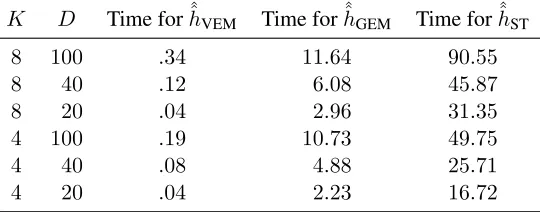
5.1 Comparison of Methods for Estimatingarg maxhm(h)
For uniformity of notation, letˆˆhST,ˆˆhVEM, andˆˆhGEMbe the estimates ofˆhformed from serial tem-pering MCMC, VI-EM, and Gibbs-EM, respectively, and recall thatˆˆhST= ˆˆh= arg maxhMcζ(h). VI-EM The estimatehˆˆVEM proposed by Blei et al. (2003) is obtained as follows. Ifh(k) is the current value ofh, the E-step of the EM algorithm is to calculate Eh(k) log(ph(ψ,w))
with respect toqφ∗. We viewQ(h)as a proxy forEh(k) log(ph(ψ,w))
, and the M-step is then to maximizeQ(h)with respect toh, to produceh(k+1). The maximization is done analytically.
The implementation of the EM algorithm through variational inference methods outlined above describes what Blei et al. (2003) doconceptually, but not exactly. Actually, Blei et al. (2003) apply VI-EM to a model that is different from ours. In that model, βis viewed as a fixed but unknown parameter, to be estimated, and the latent variable isϑ = (θ,z). Thus, the observed and missing data are, respectively,wandϑ, and the marginal likelihood is a function of two variables,handβ. Abstractly speaking, the description of VI-EM given above is exactly the same. We implemented VI-EM to the version of the LDA model considered in this paper, by modifying the Blei et al. (2003) code. While VI-EM can handle very large corpora with many topics, there are no theoretical results regarding convergence of the sequenceh(k)toarg max
hm(h), and VI-EM has the following problems: it may have poor performance if the approximation ofνh(k),wbyqφ∗ is not good; and if the likelihood surface is multimodal, as in Figure 7(e), then it can fail to find the global maximum (as is the case for all EM-type algorithms and also gradient-based approaches).
Gibbs-EM Monte Carlo EM (MC-EM), in which the E-step is replaced by a Monte Carlo estimate, dates back to Wei and Tanner (1990), and was introduced to the machine learning community in Andrieu et al. (2003). As mentioned earlier, since an error is introduced at every iteration, there is no reason to expect that the algorithm will converge at all, let alone to the true maximizer of the likelihood. In fact, Wei and Tanner (1990) recognized this problem and suggested that the Markov chain length be increased at every iteration of the EM algorithm. We will letmkdenote the MC length at thekth iteration. Convergence of MC-EM (of which the Gibbs-EM algorithm of Wallach (2008) is a special case) is a nontrivial issue. It was studied by Fort and Moulines (2003), who showed that a minimal condition is thatmk→ ∞at the rate ofka, for somea >1. However, they do not give guidelines for choosinga. Other conditions imposed in Fort and Moulines (2003) are fairly stringent, and it is not clear whether they are satisfied in the LDA model. In the current imple-mentation of Gibbs-EM (Wallach, 2006), the latent variable is taken to bez(because the standard Markov chain used to estimate posterior distributions in this model is the CGS). At thekth itera-tion, a Markov chainz1, . . . ,zmk with invariant distribution equal to the posterior distribution ofz
givenwis generated, and the functionG(h) = (1/mk)Pmk
i=1log(ph(zi,w))must be maximized. This is done by solving the equation∇G(h) = 0 using fixed-point iteration, and because∇G(h) is computationally intractable, an approximation (Minka, 2003) is used (in effect, a lower bound to G(h)is found, and the lower bound is what is maximized). This approximation introduces a second potential problem for Gibbs-EM. A third potential problem is that, as for VI-EM, the iterations may get stuck near a local maximum when the likelihood surface is multimodal.