Considering Cost Asymmetry in Learning Classifiers

Considering Cost Asymmetry in Learning Classifiers

Francis R. Bach [email protected]

Centre de Morphologie Math´ematique Ecole des Mines de Paris

35, rue Saint Honor´e 77300 Fontainebleau, France

David Heckerman [email protected]

Eric Horvitz [email protected]

Microsoft Research Redmond, WA 98052, USA

Editor: John Shawe-Taylor

Abstract

Receiver Operating Characteristic (ROC) curves are a standard way to display the performance of a set of binary classifiers for all feasible ratios of the costs associated with false positives and false negatives. For linear classifiers, the set of classifiers is typically obtained by training once, holding constant the estimated slope and then varying the intercept to obtain a parameterized set of classifiers whose performances can be plotted in the ROC plane. We consider the alternative of varying the asymmetry of the cost function used for training. We show that the ROC curve obtained by varying both the intercept and the asymmetry, and hence the slope, always outperforms the ROC curve obtained by varying only the intercept. In addition, we present a path-following algorithm for the support vector machine (SVM) that can compute efficiently the entire ROC curve, and that has the same computational complexity as training a single classifier. Finally, we provide a theoretical analysis of the relationship between the asymmetric cost model assumed when training a classifier and the cost model assumed in applying the classifier. In particular, we show that the mismatch between the step function used for testing and its convex upper bounds, usually used for training, leads to a provable and quantifiable difference around extreme asymmetries.

Keywords: support vector machines, receiver operating characteristic (ROC) analysis, linear

clas-sification

1. Introduction

Receiver Operating Characteristic (ROC) analysis has seen increasing attention in the recent statis-tics and machine-learning literature (Pepe, 2000; Provost and Fawcett, 2001; Flach, 2003). The ROC is a representation of choice for displaying the performance of a classifier when the costs as-signed by end users to false positives and false negatives are not known at the time of training. For example, when training a classifier for identifying cases of undesirable unsolicited email, end users may have different preferences about the likelihood of a false negative and false positive. The ROC curve for such a classifier reveals the ratio of false negatives and positives at different probability thresholds for classifying an email message as unsolicited or normal email.

Mercer kernels (Sch ¨olkopf and Smola, 2002). That is, given data x∈Rd, d >1, we consider classifiers of the form f(x) =sign(w>x+b), where w_∈Rd and b_∈Rare referred to as the slope and the intercept. To date, ROC curves have been usually constructed by training once, holding constant the estimated slope and varying the intercept to obtain the curve. In this paper, we show that, while that procedure appears to be the most practical thing to do, it may lead to classifiers with poor performance in some parts of the ROC curve.

The crux of our approach is that we allow the asymmetry of the cost function to vary, that is, we vary the ratio of the cost of a false positive and the cost of a false negative. For each value of the ratio, we obtain a different slope and intercept, each optimized for this ratio. In a naive implementation, varying the asymmetry would require a retraining of the classifier for each point of the ROC curve, which would be computationally expensive. In Section 3.1, we present an algorithm that can compute the solution of a support vector machine (SVM) (see, for example, Sch ¨olkopf and Smola, 2002; Shawe-Taylor and Cristianini, 2004) for all possible costs of false positives and false negatives, with the same computational complexity as obtaining the solution for only one cost function. The algorithm extends to asymmetric costs the algorithm of Hastie et al. (2005) and is based on path-following techniques that take advantage of the piecewise linearity of the path of optimal solutions. In Section 3.2, we show how the path-following algorithm can be used to obtain ROC curves. In particular, by allowing both the asymmetry and the intercept to vary, we can obtain better ROC curves than by methods that simply vary the intercept.

In Section 4, we provide a theoretical analysis of the relationship between the asymmetry of costs assumed in training a classifier and the asymmetry desired in its application. In particular, we show that, even in the population (i.e., infinite sample) case, the use of a training loss function which is a convex upper bound on the true or testing loss function (a step function) creates classifiers with sub-optimal accuracy. We quantify this problem around extreme asymmetries for several classical convex-upper-bound loss functions, including the square loss and the erf loss, an approximation of the logistic loss based on normal cumulative distribution functions (also referred to as the “error function,” and usually abbreviated as erf). The analysis is carried through for Gaussian and mixture of Gaussian class-conditional distributions (see Section 4 for more details). The main result of this analysis is that given an extreme user-defined testing asymmetry, the training asymmetry should almost always be chosen to be less extreme.

As we shall see, the consequences of the potential mismatch between the cost functions as-sumed in testing versus training underscore the value of using the algorithm that we introduce in Section 4.3. Even when costs are known (i.e., when only one point on the ROC curve is needed), the classifier resulting from our approach, which builds the entire ROC curve, is never less accurate and can be more accurate than one trained with the known costs using a convex-upper-bound loss function. Indeed, we show in Section 4.3 that computing the entire ROC curve using our algorithm can lead to substantial gains over simply training once.

2. Problem Overview

Given data x_∈Rdand labels y_{∈ {−}1,1_}, we consider linear classifiers of the form f(x) =sign(w>x+ b), where w is the slope of the classifier and b the intercept. A classifier is determined by the pa-rameters(w,b)_∈Rd+1. In Section 2.1, we introduce notation and definitions; in Section 2.2, we lay out the necessary concepts of ROC analysis, while in Section 2.3, we describe how these classifiers and ROC curves are typically obtained from data.

2.1 Asymmetric Cost and Loss Functions

Positive (resp. negative) examples are those for which y=1 (resp. y=₋1). The two types of misclassification, false positives and false negatives, are assigned two different costs. We let C+

denote the cost of a false negative and C₋ the cost of a false positive. The total expected cost is equal to

R(C+,C−,w,b) =C+P{w>x+b<0, y=1}+C−P{w>x+b>0, y=−1}.

In the context of large margin classifiers (see, for example, Bartlett et al., 2004), the expected cost is usually expressed in terms of the 0–1 loss function; indeed, if we letφ0−1(u) =1u<0 be the 0–1

loss, we can write the expected cost as

R(C+,C−,w,b) =C+E{1y=1φ0−1(w>x+b)}+C−E{1y=−1φ0−1(−w>x−b)},

where E denotes the expectation with respect to the joint distribution of(x,y).

The expected cost defined using the 0–1 loss is the cost that end users are usually interested in during the use of the classifier, while the other cost functions that we define below are used solely for training purposes. The convexity of these cost functions makes learning algorithms convergent without local minima, and leads to attractive asymptotic properties (Bartlett et al., 2004).

A traditional set-up for learning linear classifiers from labeled data is to consider a convex upper boundφon the 0–1 lossφ0−1, and to use the expectedφ-cost:

R_φ(C+,C−,w,b) =C+E{1y=1φ(w>x+b)}+C−E{1y=−1φ(−w>x−b)}.

We refer to the ratio C+/(C₋+C+)as the asymmetry. We shall use training asymmetry to refer to

the asymmetry used for training a classifier using aφ-cost, and the testing asymmetry to refer to the asymmetric cost characterizing the testing situation (reflecting end user preferences) with the actual cost based on the 0–1 loss. In Section 4, we will show that these may be different in the general case.

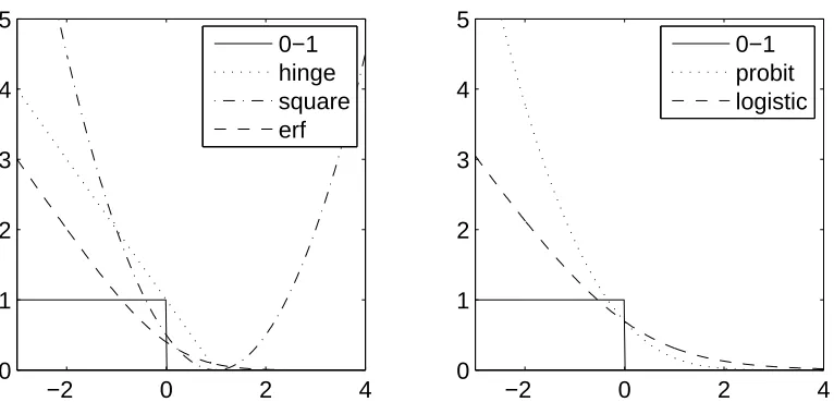
We shall consider several common loss functions. Some of the loss functions (square loss, hinge loss) lead to attractive computational properties, while others (square loss, erf loss) are more amenable to theoretical manipulations (see Figure 1 for the plot of the loss functions, as they are commonly used and defined below1):

• square loss :φsq(u) =1₂(u−1)2; the classifier is equivalent to linear regression on y,

• hinge loss : φhi(u) =max{1−u,0}; the classifier is the support vector machine (Shawe-Taylor and Cristianini, 2004),

−2 0 2 4 0

1 2 3 4 5

−2 0 2 4 0

1 2 3 4 5 0−1

hinge square erf

0−1 probit logistic

Figure 1: Loss functions. Left: plain: 0–1 loss; dotted: hinge loss, dashed: erf loss, dash-dotted: square loss. Right: plain: 0–1 loss, dotted: probit loss, dashed: logistic loss.

• erf loss : φer f(u) = [uψ(u)−u+ψ0(u)], whereψis the cumulative distribution of the stan-dard normal distribution, that is : ψ(v) = _√1

2π Rv

−∞e−t

2_/2

dt, andψ0(v) = _√1 2πe−

v2_/2

. The erf loss can be used to provide a good approximation of the logistic lossφlog(u) =log(1+e−u) as well as its derivative, and is amenable to closed-form computations for Gaussians and mix-ture of Gaussians (see Section 4 for more details). Note that the erf loss is different from the

probit loss₋logψ(u), which leads to probit regression (Hastie et al., 2001).

2.2 ROC Analysis

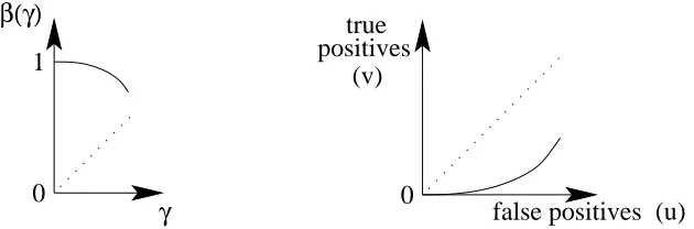
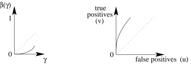
The aim of ROC analysis is to display in a single graph the performance of classifiers for all possible costs of misclassification. In this paper, we consider sets of classifiers fγ(x), parameterized by a variableγ_∈R(γcan either be the intercept or the training asymmetry).

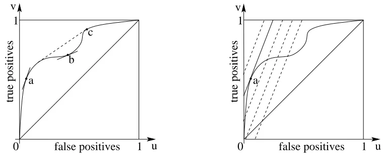
For a classifier f(x), we can define a point(u,v)in the “ROC plane,” where u is the proportion of false positives u=P(f(x) =1_|y=₋1), and v is the proportion of true positives v=P(f(x) = 1_|y=1). Whenγis varied, we obtain a curve in the ROC plane, the ROC curve (see Figure 2 for an example). Whetherγis the intercept or the training asymmetry, the ROC curve always passes through the point (0,0) and(1,1), which corresponds to classifying all points as negative (resp. positive).

The upper convex envelope of the curve is the set of optimal ROC points that can be achieved by the set of classifiers; indeed, if a point in the envelope is not one of the original points, it must lie in a segment between two points(u(γ0),v(γ0))and(u(γ1),v(γ1)), and all points in a segment between

c v

u 1

true positives

0 false positives 1 a

b

a

u v

false positives

true positives

1

0 1

Figure 2: Left: ROC curve: (plain) regular ROC curve; (dashed) convex envelope. The points a and c are ROC-consistent and the point b is ROC-inconsistent. Right: ROC curve and dashed equi-cost lines: All lines have direction(p+C+,p−C−), the plain line is optimal

and the point “a” is the optimal classifier.

only interested in the testing cost, which is a weighted linear combination of the true positive and false positive rates, the lowest testing cost is always achieved by both of these two classifiers (see Section 4.3 for an example of such a situation).

Denoting p+=P(y=1)and p−=P(y=−1), the expected(C+,C−)-cost for a classifier(u,v)

in the ROC space, is simply p+C+(1−v) +p−C−u, and thus optimal classifiers for the(C+,C−)

-cost can be found by looking at lines of slope that are normal to the direction (p₋C₋,₋p+C+),

which intersects the ROC curve and are as close as the point(0,1)as possible (see Figure 2). A point(u(γ),v(γ))is said to be ROC-consistent if it lies on the upper convex envelope; In this case, the tangent direction(du/dγ,dv/dγ)defines a cost(C+(γ),C−(γ))for which the classifier is

optimal (for the testing cost, which is defined using the 0–1 loss). The condition introduced earlier, namely that(du/dγ,dv/dγ)is normal to the direction(p₋C₋,₋p+C+), leads to:

p₋C₋du

dγ(γ)−p+C+ dv

dγ(γ) =0.

The optimal testing asymmetryβ(γ)defined as the ratio C+(γ)

C+(γ)+C−(γ), is thus equal to

β(γ), C+(γ)

C+(γ) +C−(γ)

= 1

1+p+

p−

dv dγ(γ)/

du dγ(γ)

. (1)

If a point(u(γ),v(γ))is ROC-inconsistent, then the quantityβ(γ) has no meaning, and such a classifier is generally useless, because, for all settings of the misclassification cost, that classifier can be outperformed by the other classifiers or a combination of classifiers. See Figure 2 for examples of ROC-consistent and ROC-inconsistent points.

they differ and quantify this difference for extreme asymmetries (i.e., close to the corner points (0,0)and(1,1)). This analysis highlights the value of generating the entire ROC curve, even when only one point is needed, as we will present in Section 4.3.

Handling ROC surfaces In this paper, we will also consider varying both the asymmetry of the cost function and the intercept, leading to a set of points in the ROC plane parameterized by two real values. Although the concept of ROC-consistency could easily be extended to ROC surfaces, for simplicity we do not consider it here. In all our experiments, those ROC surfaces are reduced to curves by computing their convex upper envelopes.

2.3 Learning From Data

Given n labeled data points(xi,yi), i=1, . . . ,n, the empirical cost is equal to

b

R(C+,C−,w,b) =

C+

n #{yi(w

>_{xi+b)<0,yi=1}+}C−

n #{yi(w

>_{xi+b)<0,yi=−1},}

where #A denotes the cardinality of the set A. The empiricalφ-cost is equal to

b

R_φ(C+,C−,w,b) =

C+

n _i

∑

>_x

i+b)) +

C₋

n _i

∑

−

φ(yi(w>xi+b)),

where

I

I

setup is to minimize the sum of the empiricalφ-cost and a regularization term _2n1_||w_||2, that is, to minimizeJbφ(C+,C−,w,b) =Rbφ(C+,C−,w,b) +2n1||w||2.

Note that the objective function is no longer homogeneous in (C+,C−); the sum C++C− is

referred to as the total amount of regularization. Thus, two end-user-defined parameters are needed to train a linear classifier: the total amount of regularization C++C− ∈R+, and the asymmetry

C+

C++C− ∈[0,1]. In Section 3.1, we show how the minimum ofJbφ(C+,C−,w,b), with respect to w and

b, can be computed efficiently for the hinge loss, for many values of(C+,C−), with a computational

cost that is within a constant factor of the computational cost of obtaining a solution for one value of(C+,C−).

Building an ROC curve from data If a sufficiently large validation set is available, we can train on the training set and use the empirical distribution of the validation data to plot the ROC curve. If sufficient validation data is not available, then we can use several (typically 10 or 25) random splits of the data and average scores over those splits to obtain the ROC scores. We can also use this approach to obtain confidence intervals (Flach, 2003).

3. Building ROC Curves for the SVM

In this section, we present an algorithm to compute ROC curves for the SVM that explores the two-dimensional space of cost parameters(C+,C₋)efficiently. We first show how to obtain optimal solutions of the SVM without solving the optimization problems many times for each value of (C+,C−). This method generalizes the results of Hastie et al. (2005) to the case of asymmetric cost

3.1 Building Paths of Classifiers

Given n data points xi, i=1, . . . ,n which belong toRd, and n labels yi_{∈ {−}1,1_}, minimizing the regularized empirical hinge loss is equivalent to solving the following convex optimization prob-lem (Sch¨olkopf and Smola, 2002):

min

w,b,ξ

∑

1 2||w||

2 _{such that ∀i, ξ}

i>0,ξi>1−yi(w>xi+b),

where Ci=C+ if yi=1 and Ci=C− if yi=−1.

Optimality conditions and dual problems We know derive the usual Karush-Kuhn-Tucker (KKT) optimality conditions (Boyd and Vandenberghe, 2003). The Lagrangian of the problem is (with dual variablesα,β_∈Rn+):

L(w,b,ξ,α,β) =

∑

Ciξi+ 1 2||w||

2₊

∑

i

αi(1−yi(w>xi+b))−ξi)−

∑

i

βiξi.

The derivatives with respect to the primal variables are

∂L

∂w=w−

∑

∂L

∂b =−

∑

∂L

∂ξi

=Ci−αi−βi,

The first set of KKT conditions corresponds to the nullity of the Lagrangian derivatives with respect to the primal variables, that is:

w=

∑

i

αiyixi,

∑

i

αiyi=α>y=0, _∀i,Ci=αi+βi. (2)

The slackness conditions are

∀i,αi(1−ξi+yi(w>xi+b)) =0 and βiξi=0. (3)

Finally the dual problem can be obtained by computing the minimum of the Lagrangian with respect to the primal variables. If we let denote K the n_×n Gram matrix of inner products, that is, defined by Ki j=x>_i xj, andKe=Diag(y)K Diag(y), the dual problem is:

max

α∈Rn−

1 2α

>_Keα+1>_{α such that α}>_{y=0, ∀i,06α}

i6Ci.

In the following, we only consider primal variables(w,b,ξ)and dual variables(α,β)that verify the first set of KKT conditions (2), which implies that w andβare directly determined byα.

Piecewise affine solutions Following Hastie et al. (2005), for an optimal set of primal-dual vari-ables(w,b,α), we can separate data points in three disjoint sets, depending on the values of yi(w>xi+ b) = (Keα)i+byi.

Margin :

M

L

Because of the slackness conditions (3), the sign of yi(w>xi+b)₋1 is linked with the location of

αiin the interval[0,Ci]. Indeed we have:

Left of margin : i_∈

L

R

In the optimization literature, the sets

L

R

M

M

L

R

∀i_∈

L

∀i∈

R

∀i_∈

M

α>_y=0.

This is a linear system with as many equations as unknowns (i.e., n+1). The real unknowns (not clamped to Cior 0) areα_M and b, and the smaller system is (zAdenotes the vector z reduced to its components in the set A and KA,Bdenotes the submatrix of K with indices in A and B):

e

K_M,Mα_M +by_M = 1_{M −}Ke_M,LCL

y>_Mα_M = ₋y>_LC_L,

whose solution is affine in C_L and thus in C.

Consequently, for known active sets, the solution is affine in C, which implies that the optimal variables(w,α,b) are piecewise affine continuous functions of the vector C. In our situation, C depends linearly on C+and C−, and thus the path is piecewise affine in(C+,C−).

Following a path The active sets (and thus the linear system) remain the same as long as all constraints defining the active sets are satisfied, that is, (a) yi(w>xi+b)−1 is positive for all i∈

R

L

M

always be found in linear time in n, if efficient convex hull algorithms are used (Avis et al., 1997). However, when we only follow a straight line in the(C+,C₋)-space, the polytope is then a segment and its extremities are trivial to find (also in linear time O(n)).

Following Hastie et al. (2005), if a solution is known for one value of(C+,C−), we can follow

the path along a line, by monitoring which constraints are violated at the boundary of the polytope that defines the allowed domain of(C+,C₋)for the given active sets.

Numerical issues Several numerical issues have to be solved before the previous approach can be made efficient and stable. Some of the issues directly follow the known issues of the simplex method for linear programming (which is itself an active set method) (Maros, 2002).

• Path initialization: In order to easily find a point of entry into the path, we look at situations

when all points are in

L

number of positive and negative training examples), which we now assume. The active sets remain unchanged as long as_∀i,yi(w>xi+b)61, that is:

∀i_∈

I

(Keδ+)i+ n+

n₋(Keδ−)i

∀i_∈

I

(Keδ+)i+

n+

n₋(Keδ−)i

,

whereδ+(resp.δ₋) is the indicator vector of the positive (resp. negative) examples.

Let us define the following two maxima: m+ =maxi∈I+

(Keδ+)i+n_n+

−(Keδ−)i

(attained at

i+) and m−=maxi∈I−

(Keδ+)i+n_n+

−(Keδ−)i

(attained at i₋). The previous conditions are equivalent to

−1+C+m−6b61−C+m+.

Thus, all points are in

L

unde-termined, between₋1+C+m− and 1−C+m+. At the boundary point C+=2/(m−+m+);

then both i+and i−are going from

L

M

Since we vary both C+ and C−we can start by following the line C+n+=C−n−and we are

thus able to avoid to solve a quadratic program to enter the path, as is done by Hastie et al. (2005) when the data sets are not perfectly balanced.

• Switching between active sets: Indices can go from

L

M

R

M

M

R

L

Empirically, when we follow a line in the plane(C+,C−), most points go from

L

R

M

R

L

M

• Efficient implementation of linear system: The use of Cholesky updating and downdating is

necessary for stability and speed (Golub and Van Loan, 1996).

• Computational complexity: Following the analysis of Hastie et al. (2005), if m is the

maxi-mum number of points in

M

It is worth noting that the complexity of obtaining one path of classifiers across one line is roughly the same as obtaining the solution for only one SVM using classical techniques such as sequential minimal optimization (Platt, 1998).

Classification with kernels The path following algorithm developed in this section immediately applies to non-linear classification, by replacing the Gram matrix defined as Ki j =x>_i xj, by any

kernel matrix K defined as Ki j=k(xi,xj), where k is a positive semi-definite kernel function

(Shawe-Taylor and Cristianini, 2004).

3.2 Constructing the ROC Curve

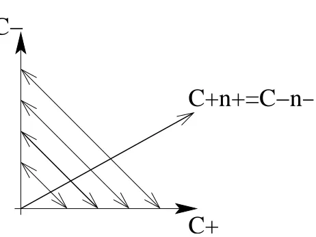
C+n+=C−n−

C+

C−

Figure 3: Lines in the(C+,C₋)-space. The line C+n+=C−n−is always followed first; then several

lines with constant C++C− are followed in parallel, around the optimal line for the

validation data (bold curve).

We assume that we have two separate data sets, one for training and one for testing. This approach generalizes to cross validation settings in a straightforward manner.

Exploration phase In order to start the path-following algorithm, we need to start at C+=C−=0

and follow the line C+n+=C−n−. We follow this line up to a large upper bound on C++C−. For

all classifiers along that line, we compute a misclassification cost on the testing set, with given asymmetry (C₊0,C₋0) (as given by the user, and usually, but not necessarily, close to a point of interest in the ROC space). We then compute the best performing pair(C₊1,C₋1)and we select pairs of the form(rC₊1,rC₋1), where r belongs to a set R of the type R=_{1,10,1/10,100,1/100, . . ._}. The set R provides further explorations for the total amount of regularization C++C−.

Then, for each r, we follow the paths of direction(1,₋1)and(₋1,1)starting from the point (rC₊1,rC1₋). Those paths have a fixed total amount of regularization but vary in asymmetry. In Figure 3, we show all of lines that are followed in the(C+,C₋)space.

Selection phase After the exploration phase, we have|R|+1 different lines in the(C+,C−)space:

the line C₋n₋=C+n+, and the|R|lines C++C−=r(C+1+C−1),r∈R. For each of these lines, we

know the optimal solution(w,b)for any cost settings on that line. The line C₋n₋=C+n+is used

for computational purposes (i.e., to enter the path), so we do not use it for testing purposes.

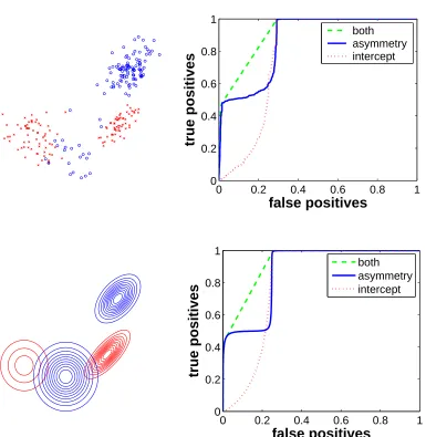
For each of the R lines in the(C+,C−)-plane, we can build the three following ROC curves, as

shown in the top of Figure 4 for a simple classification problem involving mixtures of Gaussians:

• Varying intercept: We extract the slope w corresponding to the best setting(C1

++C1−), and

• Varying asymmetry: We only consider the line C++C−=C+1+C−1 in the(C+,C−)-plane; the

classifiers that are used are the optimal solutions of the convex optimization problem. Note that for each value of the asymmetry, we obtain a different value of the slope and the intercept.

• Varying intercept and asymmetry: For each of the points on the R lines in the(C+,C−)-plane,

we discard the intercept b and keep the slope w obtained from the optimization problem; we then use all possible intercept values; this leads to R two-dimensional surfaces in the ROC plane. We then compute the convex envelope of these, to obtain a single curve.

Since all classifiers obtained by varying only the intercept (resp. the asymmetry) are included in the set used for varying both the intercept and the asymmetry, the third ROC curve always out-performs the first two curves (i.e., it is always closer to the top left corner). This is illustrated in Figure 4. Once ROC curves are obtained for each of the R lines, we can combine them by taking their upper convex envelope to obtain ROC curves obtained from even larger sets of classifiers, which span several total amounts of regularization. Note that the ROC scores that we consider are obtained by using held out testing data or cross-validation scores; thus by considering larger sets of classifiers, taking upper convex envelopes will always lead to better performance for these scores, which are only approximations of the expected scores on unseen data, and there is a potential risk of overfitting the cross-validation scores (Ng, 1997). In Section 4.3, we present empirical experiments showing that by carefully selecting classifiers based on held out data or cross-validation scores, we are not overfitting.

Intuitively, the ROC curve obtained by varying the asymmetry should be better than the ROC generated by varying the intercept because, for each point, the slope of the classifier is optimized. Empirically, this is generally true, but is not always the case, as displayed in the top of Figure 4. In the bottom of Figure 4, we show the same ROC curve, but in the infinite sample case, where the solution of the SVM was obtained by working directly with densities, separately for each training asymmetry. The ROC curve in the infinite sample case exhibit the same behavior than in the finite sample case, hinting that this behavior is not a small sample effect.

Another troubling fact is that the ROC curve obtained by varying asymmetry, exhibits strong concavities, that is, there are many ROC-inconsistent points: for those points, the solution of the SVM with the corresponding asymmetry is far from being the best linear classifier when perfor-mance is measured with the same asymmetry but with the exact 0–1 loss. In addition, even for ROC-consistent points, the training asymmetry and the testing asymmetry differ. In the next sec-tion, we analyze why they may differ and characterize their relationships in some situations.

4. Training Versus Testing Asymmetry

We observed in Section 3.2 that the training cost asymmetry can differ from the testing asymmetry. In this section, we analyze their relationships more closely for the population (i.e., infinite sample) case. Although a small sample effect might alter some of the results presented in this section, we argue that most of the discrepancies come from using a convex surrogate to the 0₋1 loss.

0 0.2 0.4 0.6 0.8 1 0

0.2 0.4 0.6 0.8 1

false positives

true positives

both asymmetry intercept

0 0.2 0.4 0.6 0.8 1 0

0.2 0.4 0.6 0.8 1

false positives

true positives

both asymmetry intercept

to the class of functions, and the best that can be hoped for is to obtain the classifier with minimal expected cost within the class of functions which is considered. Using a surrogate does not always lead to this classifier and the results of this section illustrate and quantify this fact in the context of varying cost asymmetries.

Since we are using population densities, we can get rid of the regularization term and thus only the asymmetry will have an influence on the results, that is, we can restrict ourselves to C++C−=1.

We letγ=C+/(C++C−) =C+denote the training asymmetry. For a given training asymmetryγ

and a loss functionφ, in Section 2.2, we defined the optimal testing asymmetryβ(γ)for the training asymmetryγas the testing asymmetry for which the classifier obtained by training with asymmetry

γis optimal. In this section, we will refer to theβ(γ)simply as the testing asymmetry.

Although a difference might be seen empirically for all possible asymmetries, we analyze the relationship between the testing cost asymmetry and training asymmetry in cases of extreme asym-metries, that is, in the ROC framework, close to the corner points(0,0)and(1,1). We prove that, depending on the class conditional densities, there are three possible different regimes for extreme asymmetries and that under two of these regimes, the training asymmetry should be chosen less extreme. We also provide, under certain conditions, a simple test that can determine the regime given class conditional densities.

In this section, we choose class conditional densities that are either Gaussian or a mixture of Gaussians, because (a) any density can be approximated as well as desired by mixtures of Gaus-sians (Hastie et al., 2001), and (b) for the square loss and the erf loss, they enable closed-form calculations that lead to Taylor expansions.

4.1 Optimal Solutions for Extreme Cost Asymmetries

We assume that the class conditional densities are mixtures of Gaussians, that is, the density of pos-itive (resp. negative) examples is a mixture of k+Gaussians, with means µi+and covariance matrix

Σi

+, and mixing weightsπi+, i∈ {1, . . . ,k+} (resp. k− Gaussians, with means µi− and covariance

matrixΣi

−, and mixing weightsπi−, i∈ {1, . . . ,k−}). We denote M+ (resp. M−) the d×k+ (resp.

d_×k₋) the matrix of means.

We denote p+ and p− as the marginal class densities, p+ =P(y=1), p− =P(y=−1). We

assume that all mixing weights πi_± are strictly positive, that all covariance matrices Σi_± have full rank, and that p+,p−∈(0,1).

In the following sections, we provide Taylor expansions of various quantities around the null training asymmetryγ=0. The quantities trivially extend around the reverse asymmetryγ=1. We focus on two losses, the square loss and the erf loss. The square loss, which leads to a classifier ob-tained by usual least-square linear regression on the class labels, leads to closed form computations and simple analysis. However, lossesφ(u)which remain bounded when u tends to+∞are viewed as preferable and usually lead to better performance (Hastie et al., 2001). Losses as the hinge loss or the logistic loss, which tend to zero as u tends to+∞, lead to similar performances. In order to study if using such losses might alter the qualitative behavior observed and analyzed for the square loss around extreme testing asymmetries, we use another loss with similar behavior as u tends to+∞, the erf loss. The erf loss is defined asφer f(u) = [uψ(u)−u+ψ0(u)]and leads to simpler computations than the hinge loss or the logistic loss2.

We start with an expansion of the unique global minimum(w,b)of theφ-cost with asymmetry

γ. For the square loss, (w,b) can be obtained in closed form for any class conditional densities so the expansion is easy to obtain, while for the erf loss, an asymptotic analysis of the optimality conditions has to be carried through, and is only valid for mixtures of Gaussians (see Appendix A for a proof).

We use the following usual asymptotic notations, that is, if f and g are two functions defined around x=0, with g everywhere nonnegative then, f =O(g)if and only if there exists an A positive such that_|f(x)_|6Ag(x)for all x sufficiently small, f =o(g)if and only if f(x)/g(x)tends to zero when x tends to zero, f _∼g if and only if f(x)/g(x)tends to one when x tends to zero.

Proposition 1 (square loss) Under previous assumptions, we have the following expansions:

w(γ) = 2p+

p₋γΣ

−1

− (µ+−µ−) +O(γ2),

b(γ) = ₋1+p+

p₋γ[2−2µ

>

−(µ+−µ−)] +O(γ2),

where m=µ+−µ−, andΣ± and µ±are the class conditional means and covariance matrices. For

mixtures of Gaussians, we haveΣ_±=∑iπi_±Σi_±+M±(diag(π±)−π±π>±)M>± and µ±=∑iπi_±µi_±.

Proposition 2 (erf loss) Under previous assumptions, we have the following expansions:

w(γ) = (2 log(1/γ))−1/2eΣ−₋1(˜µ+−˜µ−) +o

log(1/γ)−1/2,

b(γ) = ₋(2 log(1/γ))1/2+olog(1/γ)1/2,

with ˜m=µ+−˜µ−, ˜µ−=∑iξiµi₋ and eΣ−=∑iξiΣi₋, whereξ∈Rn+ verifies ∑iξi=1 and ξis the unique solution of a convex optimization problem defined in Appendix A.

Note that when there is only one mixture component (Gaussian densities), thenξ1 =1, and the

expansion obtained in Proposition 2 has a simpler expression similar to the one from Proposition 1. The previous propositions provide a closed-form expansion of the solutions of the convex opti-mization problems defined by the square loss and the erf loss. In the next section, we compute the testing costs using those classifiers.

4.2 Expansion of Testing Asymmetries

Using the expansions of Proposition 1 and 2, we can readily derive an expansion of the ROC coordinates for small γ, as well as the testing asymmetryβ(γ). We have (see Appendix B for a proof):

Proposition 3 (square loss) Under previous assumptions, we have the following asymptotic

expan-sion:

log

p₋ p+(β(γ)

−1 −1)

=A p

2 −

8p2₊ 1

γ2+o(1/γ

2_),

where

A= max

i₋

1

m>Σ−₋1Σi− −Σ−−1m

−max

i+

1

m>Σ−₋1Σi+ +Σ−−1m

!

γ

1

0

β(γ)

positives

(u) (v)

0

false positives true

Figure 5: Case A<0: (left) plot of the optimal testing asymmetryβ(γ)as a function of the train-ing asymmetryγ, (right) ROC curve around (0,0) as γvaries close to zero. Classifiers corresponding toγclose to zero are ROC-inconsistent.

Proposition 4 (erf loss) Under previous assumptions, we have the following asymptotic expansion:

log

p₋ p+(β(γ)

−1 −1)

=2A loge (1/γ) +o(log(1/γ)), (4)

where

e

A= max

i−

1

˜

m>eΣ−₋1Σi₋−eΣ−₋1m˜ −maxi+

1

˜ m>_eΣ−1

− Σ

i+ +Σe−−1m˜

!

.

The rest of the analysis is identical for both losses and thus, for simplicity, we focus primarily on the square loss. For the square loss, we have two different regimes, depending on the sign of

A= max

i−

1

m>Σ−₋1Σi− −Σ−−1m

−max

i+

1

m>Σ−₋1Σi+ +Σ−−1m

! :

• A<0: from the expansion in Eq. (3), we see that logp−

p+(β(γ)−1−1)

is asymptotically

equivalent to a negative constant times 1/γ2, implying that the testing asymmetryβ(γ)tends to one exponentially fast. In addition, from Eq. (1), p−

p+(β(γ)−1−1)is equal to

dv/dγ

du/dγ, which is the slope of the ROC curve. Because this is an expansion around the null training asymmetry, the ROC curve must be starting from the point (0,0); since the slope at that point is zero, that is, proportional to the horizontal axis, the ROC curve is on the bottom right part of the main diagonal and the points corresponding to training asymmetries close toγ=0 are not ROC-consistent, that is, the classifiers with training asymmetry too close to zero are useless as they are too extreme. See Figure 5 for a plot of the ROC curve around (0,0) and ofβ(γ)around

γ=0. In this situation, better performance for a given testing asymmetry can be obtained by using a less extreme training asymmetry, simply because too extreme training asymmetries lead to classifier who perform worse than trivial classifiers.

γ

1

0

β(γ)

positives (v)

(u) 0

false positives true

Figure 6: Case A>0. Left: Plot of the optimal testing asymmetryβ(γ)as a function of the training asymmetryγ; Right: ROC curve around (0,0) asγvaries close to zero. Classifiers corre-sponding toγclose to zero are ROC-consistent, but sinceβ(γ)<γ, best performance for a given testing asymmetry is obtained for less extreme training asymmetries.

around (0,0) and ofβ(γ)around zero. In this situation, better performance for a given testing asymmetry can be obtained by using a less extreme training asymmetry.

• A=0: the asymptotic expansion does not provide any information relating to the behavior of the testing asymmetry. We are currently investigating higher-order expansions in order to study the behavior of this limiting case. Given two random class-conditional distributions, this regime is unlikely. Precise measure theoretic statements regarding conditions under which the measure of the set of pairs of class-conditional distributions that belong to this regime is zero, are beyond the scope of this paper.

Note that when the two class conditional densities are Gaussians with identical covariance (a case where the Bayes optimal classifier is indeed linear for all asymmetries), we are in the present case.

Overall, in the two more likely regimes where A₆=0, we have shown that, given an extreme test-ing asymmetry, the traintest-ing asymmetry should be chosen less extreme. Because we have considered mixtures of Gaussians, this result applies to a wide variety of distributions. Moreover, this result is confirmed empirically in Section 4.3, where we show in Table 2 examples of the mismatch between testing asymmetry and training asymmetry. Moreover, the strength of the effects we have described above depends on the norm of m=µ+−µ−: if m is large, that is, the classification problem is

simple, then those effects are less strong, while when m is small, they are stronger.

For the erf loss, there are also three regimes, but with weaker effects since the testing asymmetry

β(γ)tends to zero or one polynomially fast, instead of exponentially fast. However, the qualitative result remains the same: there is a mismatch between testing and training asymmetries.

0 0.2 0.4 0.6 0.8 1 0

0.2 0.4 0.6 0.8 1

training asymmetry

testing asymmetry

0 0.2 0.4 0.6 0.8 1 0.2

0.4 0.6 0.8 1

training asymmetry

testing asymmetry

0 0.2 0.4 0.6 0.8 1 0

0.2 0.4 0.6 0.8 1

training asymmetry

testing asymmetry

0 0.2 0.4 0.6 0.8 1 0

0.2 0.4 0.6 0.8 1

training asymmetry

testing asymmetry

0 0.2 0.4 0.6 0.8 1 0

0.2 0.4 0.6 0.8 1

training asymmetry

testing asymmetry

0 0.2 0.4 0.6 0.8 1 0.2

0.4 0.6 0.8 1

training asymmetry

testing asymmetry

0 0.2 0.4 0.6 0.8 1 0

0.2 0.4 0.6 0.8 1

training asymmetry

testing asymmetry

0 0.2 0.4 0.6 0.8 1 0

0.2 0.4 0.6 0.8 1

training asymmetry

testing asymmetry

the corners. However, in general, for non-extreme asymmetries, the mismatch might be inverted, that is, a more extreme training asymmetry might lead to better performance.

Although the results presented in this section show that there are two regimes, given data, they do not readily provide a test to determine which regime is applicable and compute the corresponding optimal training asymmetry for a given testing asymmetry; an approach similar to the one presented by Tong and Koller (2000) could be followed, that is, we could estimate class conditional Gaussian mixture densities and derive the optimal hyperplane from those densities using the tests presented in this paper (which can be performed in closed form for the square loss, while for the erf loss, they require to solve a convex optimization problem). However, this approach would only applicable to extreme asymmetries (where the expansions are valid). Instead, since we have developed an efficient algorithm to obtain linear classifiers for all possible training asymmetries, it is simpler to choose among all asymmetries the one that works best for the problem at hand, which we explore in the next section.

4.3 Building the Entire ROC Curve for a Single Point

As shown empirically in Section 3.2, and demonstrated theoretically in the previous section, training and testing asymmetries may differ; this difference suggests that even when the user is interested in only one cost asymmetry, the training procedure should explore more cost asymmetries, that is, build the ROC curve as presented in Section 3.2 and chose the best classifier as follows: a given testing asymmetry leads to a unique slope in the ROC space, and the optimal point for this asymmetry is the point on the ROC curve whose tangent has the corresponding slope and which is closest to the upper-left corner. In our simulations, we compare two types of ROC curves, one which is obtained by varying the intercept, and one which is obtained by varying both the training asymmetry and the intercept. In our context, using the usual ROC curve obtained by varying only the intercept is essentially equivalent to the common practice of keeping the slope optimized with the convex risk and optimizing the intercept directly using the 0-1 loss instead of the convex surrogate (which is possible by grid search since only one real variable is considered for optimization).

We thus compare in Table 1 and 2, for various data sets and linear classifiers, and for all testing cost asymmetries3γ, the three different classifiers: (a) the classifier obtained by optimizing the con-vex risk with training cost asymmetryγ(a classifier referred to as “one”), (b) the classifier selected from the ROC curve obtained from varying the intercept of the previous classifier (a classifier re-ferred to as “int”), and (c) the classifier selected from the ROC curve obtained by varying both the training asymmetry and the intercept (a classifier referred to as “all”).

The ROC curves are obtained by 10-fold cross validation with a wrapper approach to handle the selection of the training asymmetries. The goals of these simulations are to show (1) that using only an approximation to the performance on unseen data is appropriate to select classifiers, and (2) that the performance can be significantly enhanced by simply looking at more training asymmetries. We use several data sets from the UCI data set repository (Blake and Merz, 1998), as well as the mixture of Gaussians shown in Figure 4 and the first Gaussian density in Figure 7.

We used the following wrapper approach to build the ROC curves and compare the perfor-mance of the three methods by 10-fold cross validation (Kohavi and John, 1997): for each of the

10 outer folds, we select the best parameters (i.e., training asymmetry and/or intercept) by 10-fold cross validation on the training data. The best classifier for each of the two ROC curves is kept if the difference in performance with the usual classifier “one” on the ten inner folds is statistically significant, as measured by one-tailed Wilcoxon signed rank tests with 5% confidence level (Hol-lander and Wolfe, 1999). In cases where statistical significance is not found, the original classifier obtained with the training asymmetry equal to the testing asymmetry is used (in this case, the clas-sifier is identical to the clasclas-sifier “one”). The selected clasclas-sifier is then trained on the entire training data of the outer fold and tested on the corresponding testing data. We thus obtain for each outer fold, the performance of the three classifiers (“one”, “int”,“all”).

In Table 1, we report the results of statistical tests performed to compare the three classifiers. For each testing asymmetry, we performed one-tailed Wilcoxon signed rank tests on the testing costs of the outer folds, with 5% confidence levels (Hollander and Wolfe, 1999). The proportions of acceptance (i.e., the number of acceptances divided by the number of testing asymmetries that are considered) for all one-sided tests are reported in Table 1. The empirical results from columns “all>one” and “int>one” show that comparing classifiers with only an approximation of the testing cost on unseen data, namely cross-validation scores, leads to classifiers that most of the time per-form no worse than the usual classifier (based only on the testing asymmetry and the convex risk), which strongly suggests that we are not overfitting the cross-validation data. Moreover, the column “one>int” shows that there is a significant gain in simply optimizing the intercept using the non-convex non-differentiable risk based on the 0-1 loss, and columns “one>all” and “int>all” show that there is even more gain in considering all training asymmetries4. As mentioned earlier, when the increase of performance of the classifiers “all” and “int” is not deemed statistically significant on the inner cross-validation folds, the classifier “one” is used instead. It is interesting to note that, when we do not allow the possibility to keep ”one”, we obtain significantly worse performance on the outer-fold tests

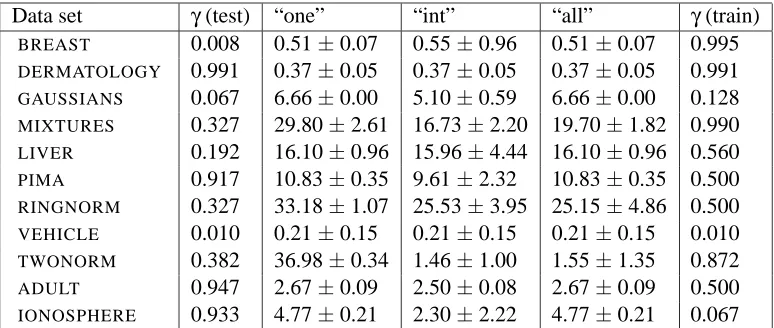
To highlight the potential difference between testing and training asymmetries, Table 2 gives some examples of mismatches between the testing asymmetry and the training asymmetry selected by the cross validation procedure. Since the training asymmetries corresponding to a given testing asymmetry may differ for each outer fold, we use the training asymmetry that was selected by the first (i.e., a random) outer fold of cross validation, and compute the cross-validation scores corresponding to this single training asymmetry for all nine other outer folds. For each data set, testing asymmetries were chosen so that the difference in testing performance between the classifier “one” and “all” on the first fold is greatest. Note that the performance of the classifier “int” is different from the performance of “all” only if the difference was deemed significant on the outer fold used to select the training asymmetry. Results in Table 2 show that in some cases, the difference is large, and that a simple change in the training procedure may lead to substantial gains. Moreover, when the testing asymmetry is extreme, such as for the GAUSSIANand PIMAdata sets, the training asymmetry is less extreme and leads to better performance, illustrating the theoretical results of Section 4. Note also, that for other data sets, such as TWONORM or IONOSPHERE, the optimal training asymmetry is very different from the testing asymmetry: we find that using all asymmetries

Data set d n one>all all>one int>all all>int one>int int>one

BREAST 9 683 8.7 0.0 4.1 0.0 5.2 0.0

DERMATOLOGY 34 358 0.0 0.0 0.0 0.0 0.0 0.0

GAUSSIANS 2 2000 17.6 0.0 14.2 0.0 9.5 0.0

MIXTURES 2 2000 49.7 0.0 25.8 0.0 41.2 0.0

LIVER 6 345 0.0 0.0 0.0 0.0 0.0 0.0

VEHICLE 18 416 13.1 0.0 13.1 0.0 0.0 0.0

PIMA 8 768 9.2 0.0 0.0 0.0 5.6 0.0

RINGNORM 2 2000 48.6 0.0 5.9 0.0 40.4 0.0

TWONORM 2 2000 97.4 0.0 15.8 5.2 91.3 0.0

ADULT 13 2000 12.0 0.0 8.8 0.0 3.2 0.0

IONOSPHERE 33 351 42.0 0.0 13.2 0.0 22.5 0.0

Table 1: Comparison of performances of classifiers: for each data set, the number of features is d, the total number of data points is n, and the proportions of acceptance (i.e., the number of acceptances divided by the number of testing asymmetries that are considered) of the six one-sided tests between the three classifiers are given in the last six columns (Wilcoxon signed rank tests with 5% confidence level comparing cross-validation scores). Note that we compare testing by using costs, and hence better performance corresponds to smaller costs. See text for details.

Data set γ(test) “one” “int” “all” γ(train)

BREAST 0.008 0.51±0.07 0.55±0.96 0.51±0.07 0.995

DERMATOLOGY 0.991 0.37_±0.05 0.37_±0.05 0.37_±0.05 0.991

GAUSSIANS 0.067 6.66_±0.00 5.10_±0.59 6.66_±0.00 0.128

MIXTURES 0.327 29.80±2.61 16.73±2.20 19.70±1.82 0.990

LIVER 0.192 16.10_±0.96 15.96_±4.44 16.10_±0.96 0.560

PIMA 0.917 10.83_±0.35 9.61_±2.32 10.83_±0.35 0.500

RINGNORM 0.327 33.18±1.07 25.53±3.95 25.15±4.86 0.500

VEHICLE 0.010 0.21_±0.15 0.21_±0.15 0.21_±0.15 0.010

TWONORM 0.382 36.98_±0.34 1.46_±1.00 1.55_±1.35 0.872

ADULT 0.947 2.67±0.09 2.50±0.08 2.67±0.09 0.500 IONOSPHERE 0.933 4.77_±0.21 2.30_±2.22 4.77_±0.21 0.067

Table 2: Training with the testing asymmetryγversus training with all cost asymmetries: we report cross-validation testing costs (multipled by 100). Only the asymmetry with the largest difference in testing performance between the classifier “one” and “all” is reported. We also report the training asymmetry which led to the best performance. Given an asymmetry

γwe use the cost settings C+=2γ, C−=2(1−γ)(which leads to the misclassification error

leads to better performance. However, we have not identified general rules for selecting the best training asymmetry.

5. Conclusion

We have presented an efficient algorithm to build ROC curves by varying the training cost asym-metries for SVMs. The algorithm is based on the piecewise linearity of the path of solutions when the cost of false positives and false negatives vary. We have also provided a theoretical analysis of the relationship between the potentially different cost asymmetries assumed in training and testing classifiers, showing that they differ under certain circumstances. In particular, in case of extreme asymmetries, our theoretical analysis suggests that training asymmetries should be chosen less ex-treme than the testing asymmetry.

We have characterized key relationships, and have worked to highlight the potential practical value of building the entire ROC curve even when a single point may be needed. All learning al-gorithms considered in this paper involve using a convex surrogate to the correct non differentiable non convex loss function. Our theoretical analysis implies that because we use a convex surro-gate, using the testing asymmetry for training leads to non-optimal classifiers. We thus propose to generate all possible classifiers corresponding to all training asymmetries, and select the one that optimizes a good approximation to the true loss function on unseen data (i.e., using held out data or cross validation). As shown in Section 3, it turns out that this can be done efficiently for the support vector machine. Such an approach can lead to a significant improvement of performance with little added computational cost.

Finally, we note that, although we have focused in this paper on the single kernel learning problem, our approach can be readily extended to the multiple kernel learning setting (Bach et al., 2005b) with appropriate numerical path following techniques.

Acknowledgments

We thank John Platt for sharing his experiences and insights with considerations of cost functions in training and testing support vector machines.

Appendix A. Proof of Expansion of Optimal Solutions

In this appendix, we give the proof of the expansions of optimal solutions for extreme

asymme-tries, for the square and erf loss. We perform the expansions using the variable ρ(γ) = C+p+

C₋p₋ =

γp+

(1₋γ)p₋ =

γp+

p₋ +O(γ

A.1 Square Loss. Proof of Proposition 1.

In this case, the classifier is simply a linear regression on y and(w,b)can be obtained in closed form as the solution of the following linear system (obtained from the normal equations):

b = ρ−1

ρ+1−w

>ρµ++µ−

ρ+1 ,

ρΣ++Σ₋+ ρ

ρ+1(µ+−µ−)(µ+−µ−)

>

w = 2ρ

ρ+1(µ+−µ−),

whereΣ+andΣ₋are the class conditional means and covariance matrices.

The first two terms of the Taylor expansions aroundρ=0 (i.e., aroundγ=0) are straightforward to obtain:

w = 2ρΣ−₋1m₋2ρ2hΣ−₋1m+Σ−1

− (Σ++mm>)Σ−−1m

i

+O(ρ3_),

b = ₋1+ρh2₋2µ>₋Σ−₋1mi+O(ρ2). A.2 Erf Loss. Proof of Proposition 2.

We begin by proving Proposition 2 in the Gaussian case, where the proof is straightforward, and we then extend to the Gaussian mixture case. In order to derive optimality conditions for the erf loss, we first need to compute expectations of the erf loss and its derivatives for Gaussian densities.

A.2.1 EXPECTATION OF THEERFLOSS ANDITSDERIVATIVES FORGAUSSIANDENSITIES

A short calculation shows that, when expectations are taken with respect to a normal distribution with mean µ and covariance matrixΣ, we have:

Eφer f(w>x+b) = (−w>µ−b)ψ

−w>µ₋b (1+w>Σw)1/2

+(1+w>Σw)1/2ψ0

−w>µ₋b (1+w>Σ_w)1/2

,

E∂φer f(w

>_x+b)

∂w = −µψ

−w>µ₋b (1+w>Σw)1/2

+ Σw

(1+w>Σw)1/2ψ

0 −w>µ−b

(1+w>Σw)1/2

,

E∂φer f(w

>_x+b)

∂b = −ψ

−w>µ₋b (1+w>Σ_w)1/2

.

A.2.2 GAUSSIANCASE

In order to derive the asymptotic expansion, we derive the optimality conditions for(w,b)and study

the behavior asρtends to zero. Let’s define t₋= w>µ−+b

(1+w>Σ₋w)1/2 and t+=

−w>µ+−b

(1+w>Σ+w)1/2.

The optimality conditions for (w,b) are the following (obtained by zeroing derivatives with respect to b and w):

p+C+

−µ+ψ(t+) + Σ+

w

(1+w>Σ+_w)1/2ψ0(t+)

+p₋C₋

µ₋ψ(t₋) + Σ−w

(1+w>Σ₋w)1/2ψ 0_(t

−)

=0,

−p+C+ψ(t+) +p−C−ψ(t−) =0.

They can be rewritten as follows (withρ=C+p+ C₋p₋):

ρ−µ+ψ(t+) + Σ+

w

(1+w>Σ+_w)1/2ψ0(t+)

+

µ₋ψ(t₋) + Σ−w

(1+w>Σ_−w)1/2ψ0(t−)

=0, (5)

ρψ(t+) =ψ(t−). (6)

Since the cumulative functionψis always between zero and one, Eq. (6) implies that asρtends to zero,ψ(t₋)tends to zero, and thus t₋tends to₋∞. This in turn implies that b/(1+_||w_||)tends to₋∞, which in turn implies that t+tends to infinity andψ(t+)tends to 1.

It is well known that as z tends to ₋∞, we haveψ(z)_≈ ψ₋0(_zz) (see, for example, Bleistein and Handelsman (1986)). Thus, if we divide Eq. (5) byψ(t₋), we get:

−ρψ_ψ(t+)

(t₋)µ++ρ

Σ+w

(1+w>Σ+_w)1/2

ψ0_(t+)

ψ(t+)

ψ(t+)

ψ(t₋)+µ−+

Σ₋w

(1+w>Σ_−w)1/2

ψ0_(t

−)

ψ(t₋) =0,that is,

Σ+w

(1+w>Σ+_w)1/2

ψ0_(t+)

ψ(t+)

+ Σ−w

(1+w>Σ_−w)1/2(−t−)∼µ+−µ−. (7)

The first term in the left hand side of Eq. (7) is the product of a bounded term and a term that goes to zero, it is thus tending to zero asρtends to zero. Since the right hand side is constant, this implies that the second term in the left hand side must be bounded, and thus, since _|t_−|tends to infinity, that w tends to zero. By removing all negligible terms in Eq. (7), we have the following expansion for w:

w_≈ 1

−t₋Σ

−1

− (µ+−µ−).

In order to obtain the expansion as a function ofρ, we need to expand t₋. From Eq. (6) and the fact thatψ(t+)tends to one, we obtain ψ(t−)∼ρ, A classical asymptotic result on the inverse erf

function shows that t_{−∼ −}p2 log(1/ρ). This finally leads to:

b(ρ) _{∼ −}(2 log(1/ρ))1/2_,

w(ρ) _∼ (2 log(1/ρ))−1/2_Σ−1

− (µ+−µ−).

A.2.3 GENERALCASE

We assume that eachπi_±is strictly positive and that each covariance matrixΣi_± is positive definite.

We define t₋i = w>µ i

−+b

(1+w>Σi

−w)1/2

and t₊i = −w>µ i

+−b

(1+w>Σi

+w)1/2

Without loss of generality, we can assume that the positive class is centered, that is, µ+ = ∑iπi+µi+=0. The optimality conditions for(w,b)are the following (obtained by zeroing derivatives

with respect to b and w):

ρ

∑

i

πi

+

−µi₊ψ(t₊i ) + Σ i

+w

(1+w>Σi

+w)1/2

ψ0_(ti

+) ! +

∑

µi₋ψ(t₋i ) + Σ

i

−w

(1+w>Σ₋w)1/2ψ 0_(ti

−)

!

=0, (8)

−ρ

∑

i

πi

+ψ(t+i) +

∑

i

πi

−ψ(t−i) =0. (9)

From Eq. (9), we obtain that ψ(t₋i ) tends to zero for all i, and this implies that b/(1+_||w_||) tends to₋∞, and in turn thatψ(t₊i )tends to 1 for all i. We can now divide Eq. (8) by∑_iπi₋ψ(t₋i ) =

ρ∑iπi+ψ(t+i ), to obtain:

∑iπi−ψ(t−i )µi−

∑iπi−ψ(t−i) −

∑iπi+ψ(t+i )µi+

∑iπi+ψ(t+i )

= ₋ 1

∑iπi+ψ(t+i )

∑

πi

+ψ(t+i )

_Σi

+w

(1+w>Σi

+w)1/2

ψ0_(ti

+)

ψ(ti

+)

−_∑ 1

iπi₋ψ(t₋i )

∑

πi

−ψ(t−i )

_Σi

−w

(1+w>Σi₋w)1/2

ψ0_(ti

−)

ψ(t₋i )

.

Let ˜π+_i = πi+ψ(t+i) ∑jπ

j

+ψ(t+j)

and ˜π−_i = πi−ψ(t−i) ∑jπ

j

−ψ(t−j)

. We can rewrite the preceding equation as

∑

i ˜

πi

−µi−−

∑

i ˜

πi

+µi+ =−

∑

i ˜ πi + _Σi +w

(1+w>Σi

+w)1/2

ψ0_(ti

+)

ψ(t₊i )

−

∑

(1+w>Σi₋w)1/2

ψ0_(ti

−)

ψ(t₋i )

.

As in the Gaussian case, the first term of the right hand is negligible compared to the second term whenρgoes to zero. Moreover, for all i, we haveψ0(t₋i )/ψ(t₋i)_{≈ −}t₋i and we thus get:

∑

i ˜

πi

−µi−−

∑

i ˜

πi

+µi+=−

∑

i ˜

πi

−

−t₋i (1+w>Σi₋w)1/2

Σi

−w. (10)

The left hand side of Eq. (10) is bounded; Because ˜π− sums to one, the lowest eigenvalue of the matrix∑_iπ˜i₋Σi₋ is lower-bounded by the smallest of the smallest eigenvalues ofΣi₋, i=1, . . . ,k₋. Thus Eq. (10) implies that t₋i w is bounded asρtends to zero. This in turn implies that w tends to zero, that b_∼t₋i for all i, and that bw is bounded.