Iterative Hessian Sketch: Fast and Accurate Solution Approximation for Constrained Least-Squares

Iterative Hessian Sketch: Fast and Accurate Solution

Approximation for Constrained Least-Squares

Mert Pilanci [email protected]

Department of Electrical Engineering and Computer Science University of California

Berkeley, CA 94720-1776, USA

Martin J. Wainwright [email protected]

Department of Electrical Engineering and Computer Science Department of Statistics

University of California

Berkeley, CA 94720-1776, USA

Editor: Tong Zhang

Abstract

We study randomized sketching methods for approximately solving least-squares problem with a general convex constraint. The quality of a least-squares approximation can be as-sessed in different ways: either in terms of the value of the quadratic objective function (cost approximation), or in terms of some distance measure between the approximate minimizer and the true minimizer (solution approximation). Focusing on the latter criterion, our first main result provides a general lower bound on any randomized method that sketches both the data matrix and vector in a least-squares problem; as a surprising consequence, the most widely used least-squares sketch is sub-optimal for solution approximation. We then present a new method known as theiterative Hessian sketch, and show that it can be used to obtain ap-proximations to the original least-squares problem using a projection dimension proportional to the statistical complexity of the least-squares minimizer, and a logarithmic number of iterations. We illustrate our general theory with simulations for both unconstrained and con-strained versions of least-squares, including `1-regularization and nuclear norm constraints. We also numerically demonstrate the practicality of our approach in a real face expression classification experiment.

Keywords: Convex optimization, Random Projection, Lasso, Low-rank Approximation, Information Theory

1. Introduction

analysis and scientific computing are constrained least-squares problems. More specifically, given a data vector y ∈ Rn, a data matrix A ∈ Rn×d and a convex constraint set C, a constrained least-squares problem can be written as follows

xLS

: = arg min

x∈C f(x) wheref(x) : =

1

2nkAx−yk22. (1) The simplest case is the unconstrained form (C = Rd), but this class also includes other interesting constrained programs, including those based `1-norm balls, nuclear norm balls, interval constraints [−1,1]d and other types of regularizers designed to enforce structure in the solution.

Randomized sketches are a well-established way of obtaining an approximate solutions to a variety of problems, and there is a long line of work on their uses (e.g., see the books and papers by Vempala (2004); Boutsidis and Drineas (2009); Mahoney (2011); Drineas et al. (2011); Kane and Nelson (2014), as well as references therein). In application to problem (1), sketching methods involving using a random matrix S ∈Rm×n to project the data matrix A and/or data vector y to a lower dimensional space (m n), and then solving the approximated least-squares problem. There are many choices of random sketching matrices; see Section 2.1 for discussion of a few possibilities. Given some choice of random sketching matrix S, the most well-studied form of sketched least-squares is based on solving the problem

e

x: = arg min x∈C

n 1

2nkSAx−Syk

2 2 o

, (2)

in which the data matrix-vector pair (A, y) are approximated by their sketched versions (SA, Sy). Note that the sketched program is an m-dimensional least-squares problem, in-volving the new data matrixSA∈_Rm×d_{. Thus, in the regimend, this approach can lead} to substantial computational savings as long as the projection dimension m can be chosen substantially less than n. A number of authors (e.g., Sarlos (2006); Boutsidis and Drineas (2009); Drineas et al. (2011); Mahoney (2011); Pilanci and Wainwright (2015a)) have inves-tigated the properties of this sketched solution (2), and accordingly, we refer to to it as the classical least-squares sketch.

There are various ways in which the quality of the approximate solution_excan be assessed. One standard way is in terms of the minimizing value of the quadratic cost functionf defining the original problem (1), which we refer to as cost approximation. In terms of f-cost, the approximate solution _ex is said to beε-optimal if

f(xLS

) ≤ f(_ex) ≤ (1 +ε)2f(xLS

). (3)

For example, in the case of unconstrained least-squares (C = Rd) with n > d, it is known that with Gaussian random sketches, a sketch size m % _ε12d suffices to guarantee that xe is

the sketch in equation (2), whereas our own past work (Pilanci and Wainwright, 2015a) provides sufficient conditions forε-accurate cost approximation of least-squares problems over arbitrary convex sets based also on the form in (2).

It should be noted, however, that other notions of “approximation goodness” are possible. In many applications, it is the least-squares minimizerxLS_{itself—as opposed to the cost value}

f(xLS_{)—that is of primary interest. In such settings, a more suitable measure of approximation} quality would be the`2-norm kex−x

LS_k

2, or the prediction (semi)-norm k_ex−xLS_k

A: = 1 √

nkA(xe−x LS_)k

2. (4)

We refer to these measures assolution approximation.

Now of course, a cost approximation bound (3) can be used to derive guarantees on the solution approximation error. However, it is natural to wonder whether or not, for a reasonable sketch size, the resulting guarantees are “good”. For instance, using arguments from Drineas et al. (2011), for the problem of unconstrained least-squares, it can be shown that the same conditions ensuring a ε-accurate cost approximation also ensure that

kx_e−xLS_k A≤ε

p

f(xLS_{). (5)}

Given lower bounds on the singular values of the data matrixA, this bound also yields control of the `2-error.

In certain ways, the bound (5) is quite satisfactory: given our normalized definition (1) of the least-squares costf, the quantityf(xLS_{) remains an order one quantity as the sample size}

ngrows, and the multiplicative factorεcan be reduced by increasing the sketch dimensionm. But how small shouldεbe chosen? In many applications of least-squares, each element of the response vector y∈_Rn _{corresponds to an observation, and so as the sample sizen increases,} we expect that xLS _{provides a more accurate approximation to some underlying population} quantity, say x∗ ∈ _Rd_{. As an illustrative example, in the special case of unconstrained} least-squares, the accuracy of the least-squares solution xLS _{as an estimate of x}∗ _{scales as} kxLS_−x∗_k

A σ 2_d

n . Consequently, in order for our sketched solution to have an accuracy of the same order as the least-square estimate, we must setε2 σ2_d

n . Combined with our earlier bound on the projection dimension, this calculation suggests that a projection dimension of the order

m% d ε2

n σ2

is required. This scaling is undesirable in the regimend, where the whole point of sketch-ing is to have the sketch dimension m much lower thann.

102 103 104 0.001

0.01 0.1 1

Row dimension n

Mean−squared error

Mean−squared error vs. row dimension

LS IHS Naive

102 103 104

0.001 0.01 0.1 1

Row dimension n

Mean−squared prediction error

Mean−squared pred. error vs. row dimension

LS IHS Naive

(a) (b)

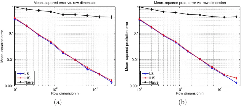
Figure 1. Plots of mean-squared error versus the row dimensionn∈ {100,200,400, . . . ,25600} for unconstrained least-squares in dimensiond= 10. The blue curves correspond to the error

xLS_−x∗ _{of the unsketched least-squares estimate. Red curves correspond to the IHS method}

applied for N = 1 +dlog(n)e rounds using a sketch size m = 7d. Black curves correspond to the naive sketch applied using M = N m projections in total, corresponding to the same number used in all iterations of the IHS algorithm. (a) Errorkx_e−x∗k2

2. (b) Prediction error kx_e−x∗k2

A=

1

nkA(xe−x ∗_)k2

2. Each point corresponds to the mean taken over 300 trials with standard errors shown above and below in crosses.

This sub-optimality holds not only for unconstrained least-squares but also more gener-ally for a broad class of constrained problems. Actugener-ally, Theorem 1 is a more general claim: any estimator based only on the pair (SA, Sy)—an infinite family of methods including the standard sketching algorithm as a particular case—is sub-optimal relative to the original least-squares estimator in the regime mn. We are thus led to a natural question: can this sub-optimality be avoided by a different type of sketch that is nonetheless computationally efficient? Motivated by this question, our second main result (Theorem 2) is to propose an alternative method—known as the iterative Hessian sketch—and prove that it yields optimal approximations to the least-squares solution using a projection size that scales with the in-trinsic dimension of the underlying problem, along with a logarithmic number of iterations. The main idea underlying iterative Hessian sketch is to obtain multiple sketches of the data (S1A, ..., SNA) and iteratively refine the solution whereN can be chosen logarithmic inn.

For the convenience of the reader, we summarize some standard notation used in this paper. For sequences {at}∞t=0 and {bt}∞t=0, we use the notationatbt to mean that there is a constant (independent oft) such thatat≤C btfor allt. Equivalently, we write btat. We write atbt ifatbtand btat.

2. Main results

In this section, we begin with background on different classes of randomized sketches, includ-ing those based on random matrices with sub-Gaussian entries, as well as those based on randomized orthonormal systems and random sampling. In Section 2.2, we prove a general lower bound on the solution approximation accuracy of any method that attempts to approx-imate the least-squares problem based on observing only the pair (SA, Sy). This negative result motivates the investigation of alternative sketching methods, and we begin this investi-gation by introducing the Hessian sketch in Section 2.3. It serves as the basic building block of the iterative Hessian sketch (IHS), which can be used to construct an iterative method that is optimal up to logarithmic factors.

2.1 Different types of randomized sketches

Various types of randomized sketches are possible, and we describe a few of them here. Given a sketching matrix S, we use {si}mi=1 to denote the collection of its n-dimensional rows. We restrict our attention to sketch matrices that are zero-mean, and that are normalized so that E[STS/m] =In.

2.1.1 Sub-Gaussian sketches:

The most classical sketch is based on a random matrixS ∈Rm×nwith i.i.d. standard Gaussian entries. A straightforward generalization is a random sketch with i.i.d. sub-Gaussian rows. In particular, a zero-mean random vectors∈_Rn_{is 1-sub-Gaussian if for anyu∈}

Rn, we have

P[hs, ui ≥εkuk2

≤e−ε2/2 for all ε≥0. (6)

For instance, a vector with i.i.d. N(0,1) entries is 1-sub-Gaussian, as is a vector with i.i.d. Rademacher entries (uniformly distributed over {−1,+1}). Suppose that we gener-ate a random matrix S ∈ _Rm×n _{with i.i.d. rows that are zero-mean, 1-sub-Gaussian, and} with cov(s) = In; we refer to any such matrix as a sub-Gaussian sketch. As will be clear, such sketches are the most straightforward to control from the probabilistic point of view. However, from a computational perspective, a disadvantage of sub-Gaussian sketches is that they require matrix-vector multiplications with unstructured random matrices. In particular, given an data matrix A ∈_Rn×d_{, computing its sketched version SA requires O(mnd) basic} operations in general (using classical matrix multiplication).

2.1.2 Sketches based on randomized orthonormal systems (ROS):

In order to define a ROS sketch, we first let H ∈ _Rn×n _{be an orthonormal matrix with} entries Hij ∈ [−√1_n,√1_n]. Standard classes of such matrices are the Hadamard or Fourier bases, for which matrix-vector multiplication can be performed inO(nlogn) time via the fast Hadamard or Fourier transforms, respectively. Based on any such matrix, a sketching matrix

S ∈Rm×n from a ROS ensemble is obtained by sampling i.i.d. rows of the form

sT =√neT_jHD with probability 1/nforj = 1, . . . , n,

where the random vector ej ∈ Rn is chosen uniformly at random from the set of all n canonical basis vectors, and D = diag(ν) is a diagonal matrix of i.i.d. Rademacher vari-ablesν ∈ {−1,+1}n_{. A similar sketching matrix can also be obtained by sampling canonical} basis vectors without replacement. Given a fast routine for matrix-vector multiplication, the sketched data (SA, Sy) can be formed in O(n dlogm) time (for instance, see Ailon and Chazelle (2006)).

2.1.3 Sketches based on random row sampling:

Given a probability distribution {pj}nj=1 over [n] = {1, . . . , n}, another choice of sketch is to randomly sample the rows of the extended data matrix A y a total of m times with replacement from the given probability distribution. Thus, the rows ofS are independent and take on the values

sT = √ej

pj

with probability pj forj= 1, . . . , n

where ej ∈ Rn is thejth canonical basis vector. Different choices of the weights {pj}nj=1 are possible, including those based on the leverage values of A—i.e.,pj ∝ kujk2 forj = 1, . . . , n, where U ∈Rn×d is the matrix of left singular vectors of A (e.g., see Drineas and Mahoney (2010)). In our analysis of lower bounds to follow, we assume that the weights areα-balanced, meaning that

max j=1,...,npj ≤

α

n (7)

for some constantα independent of n.

In the following section, we present a lower bound that applies to all the three kinds of sketching matrices described above.

2.2 Sub-optimality of classical least-squares sketch

We begin by proving a lower bound on any estimator that is a function of the pair (SA, Sy). In order to do so, we consider an ensemble of least-squares problems, namely those generated by a noisy observation model of the form

y=Ax∗+w, wherew∼N(0, σ2_I

n), (8)

the data matrix A ∈_Rn×d _{is fixed, and the unknown vector x}∗ _{belongs to some setC}

0 that is star-shaped around zero.1 _{In this case, the constrained least-squares estimate x}LS _from 1. Explicitly, this star-shaped condition means that for any x∈ C0 and scalar t ∈ [0,1], the pointtx also

equation (1) corresponds to a constrained form of maximum-likelihood for estimating the unknown regression vector x∗. In Appendix D, we provide a general upper bound on the error E[kxLS−x∗k2A] in the least-squares solution as an estimate of x

∗_{. This result provides}

a baseline against which to measure the performance of a sketching method: in particular, our goal is to characterize the minimal projection dimensionmrequired in order to return an estimate_exwith an error guaranteek_ex−xLS_k

A≈ kxLS−x∗kA. The result to follow shows that unless m≥n, then any method based on observing only the pair (SA, Sy) necessarily has a substantially larger error than the least-squares estimate. In particular, our result applies to an arbitrary measurable function (SA, Sy)7→x†, which we refer to as an estimator.

More precisely, our lower bound applies to any random matrixS ∈_Rm×n _{for which}

|||_EhST(SST)−1Si|||op≤η

m

n, (9)

whereηis a constant independent ofnandm, and|||A|||opdenotes the`2-operator norm (max-imum eigenvalue for a symmetric matrix). In Appendix A.1, we show that these conditions hold for various standard choices, including most of those discussed in the previous section. Letting BA(1) denote the unit ball defined by the semi-normk · kA, our lower bound also in-volves the complexity of the set C0∩BA(1), which we measure in terms of its metric entropy. In particular, for a given tolerance δ >0, theδ-packing numberMδ of the setC0∩BA(1) with respect tok·k_Ais the largest number of vectors{xj}M

j=1 ⊂ C0∩BA(1) such thatkxj−xkkA> δ for all distinct pairsj 6=k.

With this set-up, we have the following result:

Theorem 1 (Sub-optimality) For any random sketching matrixS ∈_Rm×n _satisfying con-dition (9), any estimator (SA, Sy)7→x† has MSE lower bounded as

sup x∗_∈C

0

ES,w

kx†−x∗k2_A

≥ σ

2 128η

log(1₂M_1/2)

min{m, n} (10)

where M_1/2 is the 1/2-packing number of C₀∩_BA(1) in the semi-norm k · k_A.

The proof, given in Appendix A, is based on a reduction from statistical minimax theory com-bined with information-theoretic bounds. The lower bound is best understood by considering some concrete examples:

Example 1 (Sub-optimality for ordinary least-squares) We begin with the simplest case— namely, in which C=Rd. With this choice and for any data matrix A with rank(A) = d, it is straightforward to show that the least-squares solution xLS _{has its prediction mean-squared}

error at most

EkxLS−x∗k2A

- σ

2_d

On the other hand, with the choice C₀ =B2(1), we can construct a 1/2-packing with M = 2d elements, so that Theorem 1 implies that any estimatorx†based on(SA, Sy)has its prediction MSE lower bounded as

ES,w

kx_b−x∗k2 A

% σ

2_d

min{m, n}. (11b)

Consequently, the sketch dimensionm must grow proportionally tonin order for the sketched solution to have a mean-squared error comparable to the original least-squares estimate. This is highly undesirable for least-squares problems in which n d, since it should be possible to sketch down to a dimension proportional to rank(A) =d. Thus, Theorem 1 this reveals a surprising gap between the classical least-squares sketch (2) and the accuracy of the original least-squares estimate.

In contrast, the sketching method of this paper, known as iterative Hessian sketching (IHS), matches the optimal mean-squared error using a sketch of size d+ log(n) in each round, and a total of log(n) rounds; see Corollary 2 for a precise statement. The red curves in Figure 1 show that the mean-squared errors (kx_b−x∗k2

2 in panel (a), andkxb−x

∗_k2

Ain panel (b)) of the IHS method using this sketch dimension closely track the associated errors of the full least-squares solution (blue curves). Consistent with our previous discussion, both curves drop off at the n−1 _rate.

Since the IHS method withlog(n)rounds uses a total ofT = log(n)d+log(n)}sketches, a fair comparison is to implement the classical method withT sketches in total. The black curves show the MSE of the resulting sketch: as predicted by our theory, these curves are relatively flat as a function of sample size n. Indeed, in this particular case, the lower bound (10)

ES,w

kx_e−x∗k2_A

% σ

2_d

m %

σ2

log2(n),

showing we can expect (at best) an inverse logarithmic drop-off. ♦

This sub-optimality can be extended to other forms of constrained least-squares estimates as well, such as those involving sparsity constraints.

Example 2 (Sub-optimality for sparse linear models) We now consider the sparse vari-ant of the linear regression problem, which involves the `0-“ball”

B0(s) : =

x∈_Rd| d X

j=1

I[xj 6= 0]≤s},

corresponding to the set of all vectors with at most s non-zero entries. Fixing some radius

R ≥ √s, consider a vector x∗∈ C₀ : =B0(s)∩ {kxk1 =R}, and suppose that we make noisy observations of the form y=Ax∗+w.

Given this set-up, one way in which to estimate x∗ is by by computing the least-squares estimate xLS _constrained2 _{to the `}

1-ball C = {x ∈ Rn | kxk1 ≤ R}. This estimator is a

form of the Lasso (Tibshirani, 1996): as shown in Appendix D.2, when the design matrix A

satisfies the restricted isometry property (see Candes and Tao (2005) for a definition), then it has MSE at most

EkxLS−x∗k2A

- σ

2_slog ed s

n . (12a)

On the other hand, the 1₂-packing number M of the set C0 can be lower bounded as logM %slog ed_s; see Appendix D.2 for the details of this calculation. Consequently, in application to this particular problem, Theorem 1 implies that any estimator x† based on the pair (SA, Sy) has mean-squared error lower bounded as

Ew,S

kx†−x∗k2_A

% σ

2_slog ed s

min{m, n} . (12b)

Again, we see that the projection dimension mmust be of the order of nin order to match the mean-squared error of the constrained least-squares estimate xLS _{up to constant factors. By}

contrast, in this special case, the sketching method developed in this paper matches the error kxLS_−x∗_k

2 using a sketch dimension that scales only asslog ed_s

+ log(n); see Corollary 3 for the details of a more general result. ♦

Example 3 (Sub-optimality for low-rank matrix estimation) In the problem of mul-tivariate regression, the goal is to estimate a matrix X∗∈_Rd1×d2 _{model based on observations} of the form

Y =AX∗+W, (13)

where Y ∈ _Rn×d1 _{is a matrix of observed responses, A ∈}

Rn×d1 is a data matrix, and

W ∈Rn×d2 _{is a matrix of noise variables. One interpretation of this model is as a} collec-tion of d2 regression problems, each involving a d1-dimensional regression vector, namely a particular column of X∗. In many applications, among them reduced rank regression, multi-task learning and recommender systems (e.g., Srebro et al. (2005); Yuan and Lin (2006); Negahban and Wainwright (2011); Bunea et al. (2011)), it is reasonable to model the matrix

X∗ as having a low-rank. Note a rank constraint on matrix X be written as an `0-“norm” constraint on its singular values: in particular, we have

rank(X)≤r if and only if

min{d1,d2} X

j=1

I[γj(X)>0]≤r,

where γj(X) denotes the jth singular value of X. This observation motivates a standard relaxation of the rank constraint using the nuclear norm |||X|||nuc: =

Pmin{d1,d2}

j=1 γj(X). Accordingly, let us consider the constrained least-squares problem

XLS

= arg min X∈Rd1×d2

n1

2|||Y −AX||| 2

fro

o

where ||| · |||fro denotes the Frobenius norm on matrices, or equivalently the Euclidean norm

on its vectorized version. Let C0 denote the set of matrices with rank r < 1₂min{d1, d2}, and Frobenius norm at most one. In this case, we show in Appendix D that the constrained least-squares solution XLS _{satisfies the bound}

E h

kXLS_−X∗_k2 A

i

- σ

2_r(d 1+d2)

n . (15a)

On the other hand, the 1₂-packing number of the setC0 is lower bounded aslogM %r d1+d2

, so that Theorem 1 implies that any estimator X† based on the pair(SA, SY) has MSE lower bounded as

Ew,S

kX†−X∗k2_A

% σ

2_{r d} 1+d2

min{m, n} . (15b)

As with the previous examples, we see the sub-optimality of the sketched approach in the regime m < n. In contrast, for this class of problems, our sketching method matches the error kXLS_−X∗_k

A using a sketch dimension that scales only as {r(d1+d2) + log(n)} log(n). See Corollary 4 for further details.

♦

2.3 Introducing the Hessian sketch

As will be revealed during the proof of Theorem 1, the sub-optimality is in part due to sketching the response vector—i.e., observing Sy instead of y. It is thus natural to con-sider instead methods that sketch only the data matrix A, as opposed to both the data matrix and data vector y. In abstract terms, such methods are based on observing the pair

SA, ATy∈_Rm×d_×

Rd. One such approach is what we refer to as the Hessian sketch— namely, the sketched least-squares problem

b

x: = arg min x∈C

n1

2kSAxk 2

2− hATy, xi

| {z }

gS(x)

o

. (16)

As with the classical least-squares sketch (2), the quadratic form is defined by the matrix

SA ∈_Rm×d_{, which leads to computational savings. Although the Hessian sketch on its own} does not provide an optimal approximation to the least-squares solution, it serves as the building block for an iterative method that can obtain an ε-accurate solution approximation in log(1/ε) iterations.

In controlling the error with respect to the least-squares solution xLS _{the set of possible} descent directions {x−xLS _{| x ∈ C} plays an important role. In particular, we define the} transformed tangent cone

KLS

=v∈_Rd |v=t A(x−xLS

Note that the error vector_bv: =A(x_b−xLS_{) of interest belongs to this cone. Our approximation} bound is a function of the quantities

Z1(S) : = inf v∈KLS_∩Sn−1

1

mkSvk

2

2 and (18a)

Z2(S) : = sup v∈KLS_∩Sn−1

hu,(

STS

m −In)vi

, (18b)

whereuis a fixed unit-norm vector. These variables played an important role in our previous analysis (Pilanci and Wainwright, 2015a) of the classical sketch (2). The following bound applies in a deterministic fashion to any sketching matrix.

Proposition 1 (Bounds on Hessian sketch) For any convex setCand any sketching ma-trix S ∈_Rm×n_{, the Hessian sketch solution}

b

x satisfies the bound

k_bx−xLS_k

A≤

Z2

Z1 kxLS_k

A. (19)

For random sketching matrices, Proposition 1 can be combined with probabilistic analysis to obtain high probability error bounds. For a given tolerance parameter ρ∈(0,1₂], consider the “good event”

E(ρ) : =

Z1≥1−ρ, and Z2 ≤

ρ

2

. (20a)

Conditioned on this event, Proposition 1 implies that

kx_b−xLS_k A≤

ρ

2 (1−ρ)kx LS_k

A ≤ ρkxLSkA, (20b)

where the final inequality holds for all ρ∈(0,1/2].

Thus, for a given family of random sketch matrices, we need to choose the projection dimension m so as to ensure the event Eρ holds for some ρ. For future reference, let us state some known results for the cases of sub-Gaussian and ROS sketching matrices. We use (c0, c1, c2) to refer to numerical constants, and we let D = dim(C) denote the dimension of the space C. In particular, we have D = d for vector-valued estimation, and D = d1d2 for matrix problems.

Our bounds involve the “size” of the cone KLS _{previously defined (17), as measured in} terms of itsGaussian width

W(KLS

) : =Eg

sup v∈KLS_∩

B2(1)

|hg, vi|

, (21)

Lemma 1 (Sufficient conditions on sketch dimension (Pilanci and Wainwright, 2015a))

(a) For sub-Gaussian sketch matrices, given a sketch size m > c0 ρ2W2(K

LS_{), we have}

PE(ρ)]≥1−c1e−c2mδ 2

. (22a)

(b) For randomized orthogonal system (ROS) sketches (sampled with replacement) over the class of self-bounding cones, given a sketch size m > c0 log4(D)

ρ2 W2(K

LS_{), we have}

PE(ρ)]≥1−c1e

−c2 mρ 2

log4(D)_{. (22b)}

The class of self-bounding cones is described more precisely in Lemma 8 of our earlier pa-per (Pilanci and Wainwright, 2015a). It includes among other special cases the cones generated by unconstrained least-squares (Example 1), `1-constrained least squares (Example 2), and least squares with nuclear norm constraints (Example 3). For these cones, given a sketch size

m > c0log4(D) ρ2 W2(K

LS_{), the Hessian sketch applied with ROS matrices is guaranteed to return}

an estimate _bxsuch that

k_bx−xLS_k

A≤ρkxLSkA (23)

with high probability. More recent work by Bourgain et al. (2015) has established sharp bounds for various forms of sparse Johnson-Lindenstrauss transforms (Kane and Nelson, 2014). As a corollary of their results, a form of the guarantee (23) also holds for such random projections.

Returning to the main thread, the bound (23) is an analogue of our earlier bound (5) for the classical sketch withpf(xLS_{) replaced bykx}LS_{kA. For this reason, we see that the Hessian} sketch alone suffers from the same deficiency as the classical sketch: namely, it will require a sketch size mnin order to mimic the O(n−1_{) accuracy of the least-squares solution.} 2.4 Iterative Hessian sketch

With this intuition in place, we now turn a precise formulation of the iterative Hessian sketch. Consider the optimization problem

b

u= arg min u∈C−xt

n1 2kAuk

2

2− hAT(y−Axt), ui o

, (24)

where xt is the iterate at step t. By construction, the optimum to this problem is given by

b

u = xLS_−xt_{. We then apply to Hessian sketch to this optimization problem (24) in order} to obtain an approximation xt+1 = xt+_bu to the original least-squares solution xLS _{that is} more accurate thanxtby a factor ρ∈(0,1/2). Recursing this procedure yields a sequence of iterates whose error decays geometrically inρ.

Formally, the iterative Hessian sketch algorithm takes the following form:

Iterative Hessian sketch (IHS):Given an iteration numberN ≥1:

(1) Initialize atx0= 0.

(2) For iterations t = 0,1,2, . . . , N − 1, generate an independent sketch matrix

St+1 ∈_Rm×n_{, and perform the update}

xt+1= arg min x∈C

n 1 2mkS

t+1_A(x−xt_)k2

2− hAT(y−Axt), xi o

. (25)

(3) Return the estimatex_b=xN.

The following theorem summarizes the key properties of this algorithm. It involves the se-quence{Z1(St), Z2(St)}N

t=1, where the quantities Z1 and Z2 were previously defined in equa-tions (18a) and (18b). In addition, as a generalization of the event (20a), we define the sequence of “good” events

Et(ρ) : =

Z1(St)≥1−ρ, and Z2(St)≤

ρ

2

fort= 1, . . . , N. (26)

With this notation, we have the following guarantee:

Theorem 2 (Guarantees for iterative Hessian sketch) The final solution x_b=xN sat-isfies the bound

kx_b−xLS_k

A≤ n_YN

t=1

Z2(St)

Z1(St) o

kxLS_k

A. (27a)

Consequently, conditioned on the event ∩N

t=1Et(ρ) for some ρ∈(0,1/2), we have

kx_b−xLS_k

Note that for any ρ ∈ (0,1/2), then event Et_{(ρ) implies that} Z2(St)

Z1(St) ≤ ρ, so that the bound (27b) is an immediate consequence of the product bound (27a).

Lemma 1 can be combined with the union bound in order to ensure that the compound event ∩N

t=1Et(ρ) holds with high probability over a sequence of N iterates, as long as the sketch size is lower bounded as m≥ c0

ρ2W2(K

LS_{) log}4_{(D) + logN. Based on the bound (27b),} we then expect to observe geometric convergence of the iterates.

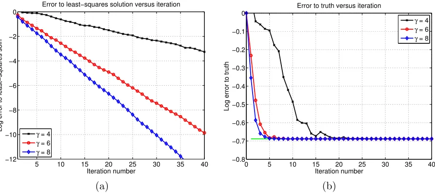
In order to test this prediction, we implemented the IHS algorithm using Gaussian sketch matrices, and applied it to an unconstrained least-squares problem based on a data matrix with dimensions (d, n) = (200,6000) and noise variance σ2 = 1. As shown in Appendix D.2, the Gaussian width of KLS _{is proportional to d, so that Lemma 1 shows that it suffices to} choose a projection dimensionm%γdfor a sufficiently large constantγ. Panel (a) of Figure 2 illustrates the resulting convergence rate of the IHS algorithm, measured in terms of the error kxt−xLS_k

A, for different values γ ∈ {4,6,8}. As predicted by Theorem 2, the convergence rate is geometric (linear on the log scale shown), with the rate increasing as the parameter γ

is increased.

5 10 15 20 25 30 35 40

−12 −10 −8 −6 −4 −2 0

Error to least−squares solution versus iteration

Iteration number

Log error to least−squares soln

γ = 4

γ = 6

γ = 8

0 5 10 15 20 25 30 35 40 −0.8

−0.7 −0.6 −0.5 −0.4 −0.3 −0.2 −0.1 0

Error to truth versus iteration

Iteration number

Log error to truth

γ = 4

γ = 6

γ = 8

(a) (b)

Figure 2. Simulations of the IHS algorithm for an unconstrained least-squares problem with noise variance σ2 _{= 1, and of dimensions (d, n) = (200,6000). Simulations based on sketch} sizes m=γd, for a parameterγ > 0 to be set. (a) Plots of the log errorkxt_−xLS_k

A versus

the iteration number t. Three different curves for γ ∈ {4,6,8}. Consistent with the theory, the convergence is geometric, with the rate increasing as the sampling factor γ is increased. (b) Plots of the log errorkxt_−x∗_k

A versus the iteration numbert. Three different curves for

γ ∈ {4,6,8}. As expected, all three curves flatten out at the level of the least-squares error kxLS_−x∗_k

A= 0.20≈ p

Assuming that the sketch dimension has been chosen to ensure geometric convergence, Theorem 2 allows us to specify, for a given target accuracyε∈(0,1), the number of iterations required.

Corollary 1 Fix some ρ∈ (0,1/2), and choose a sketch dimension m > c0log4(D) ρ2 W2(K

LS_).

If we apply the IHS algorithm forN(ρ, ε) : = 1+_log(1/ρ)log(1/ε) steps, then the outputxb=x

N _satisfies

the bound

k_bx−xLS_k

A kxLS_k

A

≤ε (28)

with probability at least 1−c1N(ρ, ε)e

−c2 mρ 2 log4(D)_.

This corollary is an immediate consequence of Theorem 2 combined with Lemma 1, and it holds for both ROS and sub-Gaussian sketches. (In the latter case, the additional log(D) terms may be omitted.) Combined with bounds on the width function W(KLS_{), it leads to} a number of concrete consequences for different statistical models, as we illustrate in the following section.

One way to understand the improvement of the IHS algorithm over the classical sketch is as follows. Fix some error toleranceε∈(0,1). Disregarding logarithmic factors, our previous results (Pilanci and Wainwright, 2015a) on the classical sketch then imply that a sketch size

m %ε−2W2_(KLS_{) is sufficient to produce a ε-accurate solution approximation. In contrast,} Corollary 1 guarantees that a sketch size m % log(1/ε) W2_(KLS_{) is sufficient. Thus, the} benefit is the reduction fromε−2 _{to log(1/ε) scaling of the required sketch size.}

It is worth noting that in the absence of constraints, the least-squares problem reduces to solving a linear system, so that alternative approaches are available. For instance, one can use a randomized sketch to obtain a preconditioner, which can then be used within the conjugate gradient method. As shown in past work (Rokhlin and Tygert, 2008; Avron et al., 2010), two-step methods of this type can lead to same reduction of ε−2 dependence to log(1/ε). However, a method of this type is very specific to unconstrained least-squares, whereas the procedure described in this paper is generally applicable to least-squares over any compact, convex constraint set.

2.5 Computational and space complexity

Let us now make a few comments about the computational and space complexity of imple-menting the IHS algorithm using the fast Johnson-Lindenstrauss (ROS) sketches, such as those based on the fast Hadamard transform. For a given sketch size m, the IHS algorithm requires O(ndlog(m)) basic operations to compute the data sketch St+1A at iteration t; in addition, it requiresO(nd) operations to computeAT(y−Axt). Consequently, if we run the algorithm for N iterations, then the overall complexity scales as

ON ndlog(m) +C(m, d)

whereC(m, d) is the complexity of solving them×ddimensional problem in the update (25). Also note that, in problems where the data matrix A is sparse, St+1A can be computed in time proportional to the number of non-zero elements inAusing Gaussian sketching matrices. The space used by the sketchesSAscales asO(md). To be clear, note that the IHS algorithm also requires access to the data via matrix-vector multiplies for forming AT(y−Axt). In limited memory environments, computing matrix-vector multiplies is considerably easier via distributed or interactive computation. For example, they can be efficiently implemented for multiple large datasets which can be loaded to memory only one at a time.

If we want to obtain estimates with accuracy ε, then we need to perform N log(1/ε) iterations in total. Moreover, for ROS sketches, we need to choose m % W2_(KLS_{) log}4_(d). Consequently, it only remains to bound the Gaussian widthWin order to specify complexities that depend only on the pair (n, d), and properties of the solution xLS_.

For an unconstrained problem with n > d, the Gaussian width can be bounded as W2_(KLS₎

- d, and the complexity of the solving the sub-problem (25) can be bounded as

d3. Thus, the overall complexity of computing anε-accurate solution scales asO(ndlog(d) +

d3) log(1/ε), and the space required is O(d2).

As will be shown in Section 3.2, in certain cases, the cone KLS _{can have substantially} lower complexity than the unconstrained case. For instance, if the solution is sparse, say withsnon-zero entries and the least-squares program involves an`1-constraint, then we have W2_(KLS₎

- slogd. Using a standard interior point method to solve the sketched problem, the total complexity for obtaining anε-accurate solution is upper bounded byO((ndlog(s) +

s2dlog2(d)) log(1/ε)). Although the sparsity s is not known a priori, there are bounds on it that can be computed in O(nd) time (for instance, see Ghaoui et al. (2011)).

3. Consequences for concrete models

In this section, we derive some consequences of Corollary 1 for particular classes of least-squares problems. Our goal is to provide empirical confirmation of the sharpness of our theoretical predictions, namely the minimal sketch dimension required in order to match the accuracy of the original least-squares solution.

3.1 Unconstrained least squares

We begin with the simplest case, namely the unconstrained least-squares problem (C=Rd). For a given pair (n, d) with n > d, we generated a random ensemble of least-square problems according to the following procedure:

• first, generate a random data matrixA∈Rn×d with i.i.d. N(0,1) entries

• second, choose a regression vector x∗ uniformly at random from the sphereSd−1 • third, form the response vectory=Ax∗+w, wherew∼N(0, σ2In) is observation noise

withσ = 1.

obtain a ε-accurate approximation to the original least-squares solution by running roughly log(1/ε)/log(1/ρ) iterations.

Now how should the toleranceεbe chosen? Recall that the underlying reason for solving the least-squares problem is to approximate x∗. Given this goal, it is natural to measure the approximation quality in terms of kxt−x∗kA. Panel (b) of Figure 2 shows the convergence of the iterates to x∗. As would be expected, this measure of error levels off at the ordinary least-squares error

kxLS_−x∗_k2 A

σ2d

n ≈0.10.

Consequently, it is reasonable to set the tolerance parameter proportional to σ2d_n, and then perform roughly 1 + log(1/ε)_log(1/ρ) steps. The following corollary summarizes the properties of the resulting procedure:

Corollary 2 For some given ρ∈(0,1/2), suppose that we run the IHS algorithm for

N = 1 +dlog √

n kxLSkA

σ log(1/ρ) e

iterations using m= c0

ρ2dprojections per round. Then the output bx satisfies the bounds

kx_b−xLS_k

A≤ r

σ2_d

n , and kx

N _−x∗_k

A≤ r

σ2_d

n +kx

LS_−x∗_k

A (30)

with probability greater than 1−c1N e

−c2 mρ 2 log4(d)_.

In order to confirm the predicted bound (30) on the error kx_b−xLS_{kA, we performed a} second experiment. Fixing n = 100d, we generated T = 20 random least squares problems from the ensemble described above with dimension dranging over{32,64,128,256,512}. By

our previous choices, the least-squares estimate should have error kxLS_−x∗_k

2≈ q

σ2_d n = 0.1 with high probability, independently of the dimensiond. This predicted behavior is confirmed by the blue bars in Figure 3; the bar height corresponds to the average over T = 20 trials, with the standard errors also marked. On these same problem instances, we also ran the IHS algorithm using m= 6dsamples per iteration, and for a total of

N = 1 +dlog p_n

d

log 2 e = 4 iterations.

SincekxLS_−x∗_k A

q σ2_d

n ≈0.10, Corollary 2 implies that with high probability, the sketched solution x_b=xN satisfies the error bound

kx_b−x∗k₂ ≤c0₀

r

σ2_d

n

16 32 64 128 256 0

0.05 0.1 0.15 0.2 0.25

Dimension

Error

Least−squares vs. dimension

Figure 3. Simulations of the IHS algorithm for unconstrained least-squares. In these experi-ments, we generated random least-squares problem of dimensionsd∈ {16,32,64,128,256}, on all occasions with a fixed sample sizen = 100d. The initial least-squares solution has error kxLS_−x∗_k

A ≈ 0.10, as shown by the blue bars. We then ran the IHS algorithm for N = 4

iterations with a sketch size m = 6d. As shown by the green bars, these sketched solutions show an error kx_b−x∗kA ≈0.11 independently of dimension, consistent with the predictions

of Corollary 2. Finally, the red bars show the error in the classical sketch, based on a sketch size M =N m= 24d, corresponding to the total number of projections used in the iterative algorithm. This error is roughly twice as large.

3.2 Sparse least-squares

We now turn to a study of an `1-constrained form of least-squares, referred to as the Lasso or relaxed basis pursuit program (Chen et al., 1998; Tibshirani, 1996). In particular, consider the convex program

xLS_{= arg min}

kxk1≤R 1

2ky−Axk 2

2 , (31)

where R >0 is a user-defined radius. This estimator is well-suited to the problem of sparse linear regression, based on the observation model y=Ax∗+w, wherex∗ has at mosts non-zero entries, andA∈_Rn×d _{has i.i.d. N(0,1) entries. For the purposes of this illustration, we} assume3 that the radius is chosen such thatR=kx∗k₁.

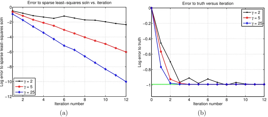
Under these conditions, the proof of Corollary 3 shows that a sketch sizem≥γ slog ed_s suffices to guarantee geometric convergence of the IHS updates. Panel (a) of Figure 4 illus-trates the accuracy of this prediction, showing the resulting convergence rate of the the IHS

3. In practice, this unrealistic assumption of exactly knowing kx∗k1 is avoided by instead considering the

algorithm, measured in terms of the error kxt−xLS_k

A, for different values γ ∈ {2,5,25}. As predicted by Theorem 2, the convergence rate is geometric (linear on the log scale shown), with the rate increasing as the parameterγ is increased.

As long asn_%slog ed_s

, it also follows as a corollary of Proposition 2 that

kxLS_−x∗_k2 A

-σ2slog ed_s

n . (32)

with high probability. This bound suggests an appropriate choice for the tolerance parameter

εin Theorem 2, and leads us to the following guarantee.

Corollary 3 For the stated random ensemble of sparse linear regression problems, suppose

that we run the IHS algorithm for N = 1 +dlog

√

nkxLSkA σ

log(1/ρ) e iterations using m = c0 ρ2slog

ed s

projections per round. Then with probability greater than 1−c1N e

−c2 mρ 2

log4(d)_{, the output} b

x

satisfies the bounds

kx_b−xLS_k

A≤ s

σ2_slog ed s

n and kx

N _−x∗_k

A≤ s

σ2_slog ed s

n +kx

LS₋

x∗kA. (33)

In order to verify the predicted bound (33) on the errorkx_b−xLS_k

A, we performed a second experiment. Fixing n = 100slog ed_s. we generated T = 20 random least squares problems (as described above) with the regression dimension ranging as d ∈ {32,64,128,256}, and sparsity s = d2√de. Based on these choices, the least-squares estimate should have error

kxLS_−x∗_k A≈

r

σ2_slog ed s

n = 0.1 with high probability, independently of the pair (s, d). This predicted behavior is confirmed by the blue bars in Figure 5; the bar height corresponds to the average over T = 20 trials, with the standard errors also marked.

On these same problem instances, we also ran the IHS algorithm using N = 4 iterations with a sketch size m = 4slog ed_s. Together with our earlier calculation of kxLS_−x∗_kA, Corollary 2 implies that with high probability, the sketched solution x_b = xN satisfies the error bound

kx_b−x∗k_A≤c0 s

σ2_slog ed s

n (34)

2 4 6 8 10 12 −12

−10 −8 −6 −4 −2 0

Error to sparse least−squares soln vs. iteration

Iteration number Log error to sparse least−squares soln γ_γ = 2 _{= 5}

γ = 25

0 2 4 6 8 10 12

−1 −0.8 −0.6 −0.4 −0.2 0

Error to truth versus iteration

Iteration number

Log error to truth

γ = 2

γ = 5

γ = 25

(a) (b)

Figure 4. Simulations of the IHS algorithm for a sparse least-squares problem with noise variance σ2 = 1, and of dimensions (d, n, s) = (256,8872,32). Simulations based on sketch sizesm=γslogd, for a parameterγ >0 to be set. (a) Plots of the log errorkxt_−xLS_k

2versus the iteration numbert. Three different curves for γ ∈ {2,5,25}. Consistent with the theory, the convergence is geometric, with the rate increasing as the sampling factor γ is increased. (b) Plots of the log errorkxt−x∗k2 versus the iteration numbert. Three different curves for γ∈ {2,5,25}. As expected, all three curves flatten out at the level of the least-squares error

kxLS_−x∗_k

2= 0.10≈

q

slog(ed/s)

n .

3.3 Some larger-scale experiments

In order to further explore the computational gains guaranteed by IHS, we performed some larger scale experiments on sparse regression problems, with the sample size n ranging over the set {212_,213_{, ...,2}19_{} with a fixed input dimension d = 500. As before, we generate} observations from the linear model y = Ax∗+w, where x∗ has at most s non-zero entries, and each row of the data matrix A ∈ _Rn×d _{is distributed i.i.d. according to a N(1}

d,Σ) distribution. Here the d-dimensional covariance matrix Σ has entries Σjk = 2×0.9|j−k|, so that the columns of the matrix A will be correlated. Setting a sparsity s = d3 log(d)e, we chose the unknown regression vectorx∗ with its support uniformly random with entries±_√1

s with equal probability.

Baseline: In order to provide a baseline for comparison, we used the homotopy algorithm— that is, the Lasso modification of the LARS updates (Osborne et al., 2000; Efron et al., 2004)— to solve the original `1 constrained problem with `1-ball radius R =

√

16 32 64 128 256 0

0.02 0.04 0.06 0.08 0.1 0.12 0.14 0.16 0.18 0.2

Dimension

Error

Sparse least squares vs. dimension

Figure 5. Simulations of the IHS algorithm for `1-constrained least-squares. In these experiments, we generated random sparse least-squares problem of dimensions

d∈ {16,32,64,128,256} and sparsity s = d2√de, on all occasions with a fixed sample size

n= 100slog ed s

. The initial Lasso solution has errorkxLS_−x∗_k

2≈0.10, as shown by the blue bars. We then ran the IHS algorithm forN = 4 iterations with a sketch size m= 4slog ed_s

. These sketched solutions show an errork_bx−x∗kA≈0.11 independently of dimension,

consis-tent with the predictions of Corollary 3. Red bars show the error in the naive sketch estimate, using a sketch of sizeM =N m= 16slog ed_s, equal to the total number of random projections used by the IHS algorithm. The resulting error is roughly twice as large.

relative to the homotopy algorithm in terms of computation time; see Bach et al. (2011) for observations of this phenomenon in past work.

IHS implementation: For comparison, we implemented the IHS algorithm with a projection dimension m =b4slog(d)c. After projecting the data, we then used the homotopy method to solve the projected sub-problem at each step. In each trial, we ran the IHS algorithm for

N =dlogne iterations.

Table 1 provides a summary comparison of the running times for the baseline method (homotopy method on the original problem), versus the IHS method (running time for com-puting the iterates using the homotopy method), and IHS method plus sketching time. Note that with the exception of the smallest problem size (n = 4096), the IHS method including sketching time is the fastest, and it is more than two times faster for large problems. The gains are somewhat more significant if we remove the sketching time from the comparison.

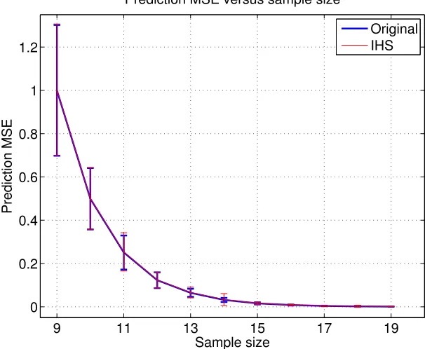
One way in which to measure the quality of the least-squares solutionxLS _{as an estimate} of x∗ is via its mean-squared (in-sample) prediction error kxLS_−x∗_k2

A =

Samplesn 4096 8192 16384 32768 65536 131072 262144 524288 Baseline 0.0840 0.1701 0.3387 0.6779 1.4083 2.9052 6.0163 12.0969

IHS 0.0783 0.0993 0.1468 0.2174 0.3601 0.6846 1.4748 3.1593 IHS+Sketch 0.0877 0.1184 0.1887 0.3222 0.5814 1.1685 2.5967 5.5792

Table 1. Running time comparison in seconds of the Baseline (homotopy method applied to original problem), IHS (homotopy method applied to sketched subproblems), and IHS plus sketching time. Each running time estimate corresponds to an average over 300 independent trials of the random sparse regression model described in the main text.

9 11 13 15 17 19

0 0.2 0.4 0.6 0.8 1 1.2

Prediction MSE versus sample size

Prediction MSE

Sample size

Original IHS

Figure 6. Plots of the mean-squared prediction errors kA(ex−x ∗_)k2

2

n versus the sample size

n ∈ 2{9,10,...,19} _{for the original least-squares solution (} e

x =xLS _{in blue) versus the sketched} solution (x_b = xLS _{in red). Each point on each curve corresponds to the average over 300} independent trials of the same type used to generate the data in Table 1; the error bars correspond to one standard errors. In generating the plots, all errors have been renormalized so that the error for sample sizen= 29 is equal to one. As can be seen, the sketched method generates solutions with prediction MSE that are essentially indistinguishable from the original solution.

dimension d and sparsity s fixed. Figure 6 compares the prediction MSE of xLS _{versus the} analogous quantitykx_b−x∗k2

3.4 Matrix estimation with nuclear norm constraints

We now turn to the study of nuclear-norm constrained form of least-squares matrix regression. This class of problems has proven useful in many different application areas, among them matrix completion, collaborative filtering, multi-task learning and control theory (e.g., (Fazel, 2002; Yuan et al., 2007; Bach, 2008; Recht et al., 2010; Negahban and Wainwright, 2012)). In particular, let us consider the convex program

XLS_{= arg min} X∈Rd1×d2

n1

2|||Y −AX||| 2 fro

o

such that |||X|||nuc≤R, (35)

where R >0 is a user-defined radius as a regularization parameter.

3.4.1 Simulated data

Recall the linear observation model previously introduced in Example 3: we observe the pair (Y, A) linked according to the linearY =AX∗+W, where the unknown matrixX∗ ∈_Rd1×d2 is an unknown matrix of rank r. The matrix W is observation noise, formed with i.i.d.

N(0, σ2) entries. This model is a special case of the more general class of matrix regression problems (Negahban and Wainwright, 2012). As shown in Appendix D.2, if we solve the nuclear-norm constrained problem with R = |||X∗|||nuc, then it produces a solution such that

E|||XLS−X∗|||2fro] - σ

2r(d1+d2)

n . The following corollary characterizes the sketch dimension and iteration number required for the IHS algorithm to match this scaling up to a constant factor.

Corollary 4 (IHS for nuclear-norm constrained least squares) Suppose that we run

the IHS algorithm for N = 1 +dlog

√

n kXLSkA σ

log(1/ρ) eiterations usingm=c0ρ 2_{r d}

1+d2

projections

per round. Then with probability greater than 1−c1N e

−c2 mρ 2

log4(d1d2), the output XN satisfies the bound

kXN −X∗kA≤ s

σ2_{r d} 1+d2

n +kX

LS₋

X∗kA. (36)

We have also performed simulations for low-rank matrix estimation, and observed that the IHS algorithm exhibits convergence behavior qualitatively similar to that shown in Figures 3 and 5. Similarly, panel (a) of Figure 8 compares the performance of the IHS and classical methods for sketching the optimal solution over a range of row sizes n. As with the uncon-strained least-squares results from Figure 1, the classical sketch is very poor compared to the original solution whereas the IHS algorithm exhibits near optimal performance.

3.4.2 Application to multi-task learning

for each separate task, but since the classification problems are so closely related, the optimal classifiers are likely to share structure. One way of capturing this shared structure is by concatenating all the different linear classifiers into a matrix, and then estimating this matrix in conjunction with a nuclear norm penalty (Amit et al., 2007; Argyriou et al., 2008).

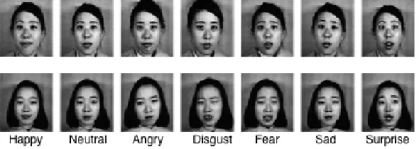
Figure 7. Japanese Female Facial Expression (JAFFE) Database: The JAFFE database consists of 213 images of 7 different emotional facial expressions (6 basic facial expressions + 1 neutral) posed by 10 Japanese female models.

In more detail, we performed a simulation study using the The Japanese Female Facial Expression (JAFFE) database (Lyons et al., 1998). It consists of N = 213 images of 7 facial expressions (6 basic facial expressions + 1 neutral) posed by 10 different Japanese female models; see Figure 7 for a few example images. We performed an approximately 80 : 20 split of the data set into ntrain = 170 training and ntest = 43 test images respectively. Then we

consider classifying each facial expression and each female model as a separate task which gives a total ofd_task = 17 tasks. For each taskj= 1, . . . , d_task, we construct a linear classifier of the form a7→ sign(ha, xji), where a ∈Rd denotes the vectorized image features given by Local Phase Quantization (Ojansivu and Heikkil, 2008). In our implementation, we fixed the number of features d= 32. Given this set-up, we train the classifiers in a joint manner, by optimizing simultaneously over the matrix X∈Rd×dtask with the classifier vectorxj ∈Rd as its jth column. The image data is loaded into the matrixA∈_Rntrain×d_{, with image feature}

vectorai ∈Rd in columnifori= 1, . . . , ntrain. Finally, the matrixY ∈ {−1,+1}ntrain×dtask

encodes class labels for the different classification problems. These instantiations of the pair (Y, X) give us an optimization problem of the form (35), and we solve it over a range of regularization radii R.

More specifically, in order to verify the classification accuracy of the classifier obtained by IHT algorithm, we solved the original convex program, the classical sketch based on ROS sketches of dimensionm= 100, and also the corresponding IHS algorithm using ROS sketches of size 20 in each of 5 iterations. In this way, both the classical and IHS procedures use the same total number of sketches, making for a fair comparison. We repeated each of these three procedures for all choices of the radius R ∈ {1,2,3, . . . ,12}, and then applied the resulting classifiers to classify images in the test dataset. For each of the three procedures, we calculated the classification error rate, defined as the total number of mis-classified images divided by ntest×dtask. Panel (b) of Figure 8 plots the resulting classification errors versus

over the randomness in generating sketching matrices. The plots show that the IHS algorithm yields classifiers with performance close to that given by the original solution over a range of regularizer parameters, and is superior to the classification sketch. The error bars also show that the IHS algorithm has less variability in its outputs than the classical sketch.

10 20 30 40 50 60 70 80 90 100

0.4 0.6 0.8 1 1.2 1.4 1.6 1.8 2 2.2 2.4

Mean−squared error vs. row dimension

Row dimension n

Mean−squared error

Original IHS Naive

2 4 6 8 10 12

0.12 0.122 0.124 0.126 0.128 0.13

Regularization parameter R

Classification error rate on test data

Classification error rate vs. regularization parameter

IHS Naive Original

(a) (b)

Figure 8. Simulations of the IHS algorithm for nuclear-norm constrained problems. The blue curves correspond to the solution of the original (unsketched problem), whereas red curves correspond to the IHS method applied for N = 1 +dlog(n)e rounds using a sketch size of

m. Black curves correspond to the naive sketch applied usingM =N mprojections in total, corresponding to the same number used in all iterations of the IHS algorithm. (a) Mean-squared error versus the row dimensionn∈[10,100] for recovering a 20×20 matrix of rankr2, using a sketch dimensionm= 60. Note how the accuracy of the IHS algorithm tracks the error of the unsketched solution over a wide range ofn, whereas the classical sketch has essentially constant error. (b) Classification error rate versus regularization parameterR∈ {1, . . . ,12}, with error bars corresponding to one standard deviation over the test set. Sketching algorithms were applied to the JAFFE face expression using a sketch dimension ofM = 100 for the classical sketch, andN = 5 iterations withm= 20 sketches per iteration for the IHS algorithm.

4. Discussion

In addition to these theoretical results, we also provided empirical evaluations that reveal the sub-optimality of the classical sketch, and show that the IHS algorithm produces near-optimal estimators. Finally, we applied our methods to a problem of facial expression using a multi-task learning model applied to the JAFFE face database. We showed that IHS algorithm applied to a nuclear-norm constrained program produces classifiers with considerably better classification accuracy compared to the naive sketch.

There are many directions for further research, but we only list here some of them. The idea behind iterative sketching can also be applied to problems beyond minimizing a least-squares objective function subject to convex constraints. Examples include penalized forms of regression, e.g., see the recent work (Yang et al., 2015), and various other cost functions. An important class of such problems are `p-norm forms of regression, based on the convex program

min

x∈_RdkAx−yk

p

p for somep∈[1,∞].

The case of`1-regression (p= 1) is an important special case, known as robust regression; it is especially effective for data sets containing outliers (Huber, 2001). Recent work (Clarkson et al., 2013) has proposed to find faster solutions of the`1-regression problem using the classical sketch (i.e., based on (SA, Sy)) but with sketching matrices based on Cauchy random vectors. Based on the results of the current paper, our iterative technique might be useful in obtaining sharper bounds for solution approximation in this setting as well. Finally, we refer the reader to the more recent work (Pilanci and Wainwright, 2015b) on sketching for general convex objective functions.

Acknowledgments

Both authors were partially supported by Office of Naval Research MURI grant N00014-11-1-0688, Office of Naval Research MURI grant ONR-MURI-DOD-002888, and National Science Foundation Grants CIF-31712-23800 and DMS-1107000. In addition, MP was supported by a Microsoft Research Fellowship.

Appendix A. Proof of lower bounds

This appendix is devoted to the verification of condition (9) for different model classes, followed by the proof of Theorem 1.

A.1 Verification of condition (9)

We verify the condition for three different types of sketches.

A.1.1 Gaussian sketches:

distributed over the sphereSn−1_{. Consequently, we have}

ES

ST SST)−1S=E m X

i=1

viviT =

m

nIn, (37)

showing that condition (9) holds withη = 1.

A.1.2 ROS sketches (sampled without replacement):

In this case, we have S =√nP HD, where P ∈Rm×n is a random picking matrix with each row being a standard basis vector sampled without replacement. We then have SST =nIm and also EP[PTP] = m_nIn, so that

ES[ST(SST)−1S] =ED,P[DHTPTP HD] =ED[DHT(

m

nIn)HD] = m

nIn,

showing that the condition holds with η= 1.

A.1.3 Weighted row sampling:

Finally, suppose that we sample m rows independently using a distribution {pj}nj=1 on the rows of the data matrix that is α-balanced (7). Letting R ⊆ {1,2, . . . , n} be the subset of rows that are sampled, and letNj be the number of times each row is sampled. We then have

E h

ST SST)−1Si=X j∈R

E[ejeTj] = D,

where D ∈ _Rn×n _{is a diagonal matrix with entries D}

jj = P[j ∈ R]. Since the trials are independent, thejthrow is sampled at least once inmtrials with probabilityqj = 1−(1−pj)m, and hence

ES

ST SST)−1S= diag {1−(1−pi)m}mi=1

1−(1−p∞)m

In mp∞,

wherep∞= maxj∈[n]pj. Consequently, as long as the row weights areα-balanced (7) so that

p∞≤ α_n, we have

|||_ES

ST SST)−1S

|||op≤α

m n

showing that condition (9) holds withη =α, as claimed.

A.2 Proof of Theorem 1

Let{zj}M

j=1be a 1/2-packing ofC0∩BA(1) in the semi-normk · kA, and for a fixedδ∈(0,1/4), definexj = 4δzj. Sine 4δ ∈(0,1), the star-shaped assumption guarantees that eachxj belongs toC0. We thus obtain a collection of M vectors in C0 such that

2δ≤ √1

nkA(x

j_−xk_)k 2

| {z }

kxj_−xk_k A

Letting J be a random index uniformly distributed over{1, . . . , M}, suppose that condition-ally on J = j, we observe the sketched observation vector Sy = SAxj +Sw, as well as the sketched matrixSA. Conditioned onJ =j, the random vectorSyfollows aN(SAxj, σ2SST) distribution, denoted byPxj. We letY denote the resulting mixture variable, with distribution

1 M

PM j=1Pxj.

Consider the multiway testing problem of determining the indexJ based on observingY. With this set-up, a standard reduction in statistical minimax (e.g., (Birg´e, 1987; Yu, 1997)) implies that, for any estimator x†, the worst-case mean-squared error is lower bounded as

sup x∗_∈CES,w

kx†−x∗k2_A≥δ2inf

ψ P[ψ(Y)6=J], (38)

where the infimum ranges over all testing functions ψ. Consequently, it suffices to show that the testing error is lower bounded by 1/2.

In order to do so, we first apply Fano’s inequality (Cover and Thomas, 1991) conditionally on the sketching matrix S to see that

P[ψ(Y)6=J] = ES n

P[ψ(Y)6=J |S] o

≥1−ES

IS(Y;J)

+ log 2

logM , (39)

whereIS(Y;J) denotes the mutual information betweenY andJ withSfixed. Our next step is to upper bound the expectationES[I(Y;J)].

Letting D(Pxj k _Pxk) denote the Kullback-Leibler divergence between the distributions

Pxj and _Pxk, the convexity of Kullback-Leibler divergence implies that

IS(Y;J) = 1

M

M X

j=1

D(Pxj k

1

M

M X

k=1

Pxk) ≤

1

M2 M X

j,k=1

D(Pxj k_Pxk).

Computing the KL divergence for Gaussian vectors yields

IS(Y;J)≤ 1

M2 M X

j,k=1 1 2σ2(x

j_−xk₎T_ATh_ST_(SST₎−1_Si_A(xj_−xk_).

Thus, using condition (9), we have

ES[I(Y;J)]≤ 1

M2 M X

j,k=1

m η

2nσ2kA(x

j_−xk_)k2 2 ≤

32m η σ2 δ

2_,

where the final inequality uses the fact that kxj−xkkA≤8δ for all pairs. Combined with our previous bounds (38) and (39), we find that

sup x∗_∈CE

kx_b−x∗k2₂ ≥δ2

n 1−32

m η δ2

σ2 + log 2 logM

o

.

Appendix B. Proof of Proposition 1

Since _bx and xLS _{are optimal and feasible, respectively, for the Hessian sketch program (16),} we have

hATST SA_bx−y

, xLS₋ b

xi ≥0 (40a)

Similarly, since xLS _and b

xare optimal and feasible, respectively, for the original least squares program

hAT(AxLS_−y), b

x−xLS_{i ≥0. (40b)}

Adding these two inequalities and performing some algebra yields the basic inequality

1

mkSA∆k

2 2 ≤ (Ax LS

)T In−

STS m A∆ . (41)

Since AxLS _{is independent of the sketching matrix andA∆∈ K}LS_{, we have}

1

mkSA∆k

2

2 ≥Z1kA∆k22, and (Ax

LS

)T In−STS

A∆

≤Z2kAx LS_k

2kA∆k2, using the definitions (18a) and (18b) of the random variables Z1 and Z2 respectively. Com-bining the pieces yields the claim.

Appendix C. Proof of Theorem 2

It suffices to show that, for each iterationt= 0,1,2, . . ., we have

kxt+1−xLS_k A≤

Z2(St+1)

Z1(St+1)

kxt−xLS_k

A. (42)

The claimed bounds (27a) and (27b) then follow by applying the bound (42) successively to iterates 1 through N.

For simplicity in notation, we abbreviateSt+1 toS andxt+1 tobx. Define the error vector ∆ = x_b−xLS_{. With some simple algebra, the optimization problem (25) that underlies the} updatet+ 1 can be re-written as

b

x= arg min x∈C

n 1

2mkSAxk

2

2− hATy, xe i o

,

where_ey: =y−hI−S_mTSiAxt_{. Since} b

xandxLS_{are optimal and feasible respectively, the usual} first-order optimality conditions imply that

hATS

T_S

m Ax−A

T e

y, xLS₋ b

xi ≥0.

As before, since xLS _{is optimal for the original program, we have}

hAT(AxLS₋ e

y+ h

I−S T_S

m

i

Axt),bx−x LS_{i ≥}

Adding together these two inequalities and introducing the shorthand ∆ =_bx−xLS _yields

1

mkSA∆k

2 2 ≤

(A(x

LS_−xt₎T

I− S T_S

m

A∆

(43)

Note that the vectorA(xLS_−xt_{) is independent of the randomness in the sketch matrixS}t+1_. Moreover, the vector A∆ belongs to the cone K, so that by the definition of Z2(St+1), we have

(A(x

LS₋

xt)T h

I−S T_S

m

i

A∆

≤ kA(x LS₋

xt)k2kA∆k2Z2(St+1). (44a) Similarly, note the lower bound

1

mkSA∆k

2

2≥ kA∆k22 Z1(St+1). (44b) Combining the two bounds (44a) and (44b) with the earlier bound (43) yields the claim (42).

Appendix D. Maximum likelihood estimator and examples

In this section, we a general upper bound on the error of the constrained least-squares estimate. We then use it (and other results) to work through the calculations underlying Examples 1 through 3 from Section 2.2.

D.1 Upper bound on MLE

The accuracy ofxLS _{as an estimate ofx}∗ _{depends on the “size” of the star-shaped set}

K(x∗) =

v∈_Rd _{|v= √}t

nA(x−x

∗_{) for some t∈[0,1] andx∈ C . (45)}

When the vectorx∗ is clear from context, we use the shorthand notation K∗ _{for this set. By}

taking a union over all possible x∗ ∈ C0, we obtain the set K : = S x∗_∈C

0

K(x∗), which plays

an important role in our bounds. The complexity of these sets can be measured of their localized Gaussian widths. For any radius ε >0 and set Θ⊆_Rn_{, the Gaussian width of the} set Θ∩B2(ε) is given by

Wε(Θ) : =Eg h

sup θ∈Θ

kθk2≤ε

|hw, θi|i, (46a)

whereg∼N(0, In×n) is a standard Gaussian vector. Whenever the set Θ is star-shaped, then

it can be shown that, for anyσ >0 and positive integer`, the inequality

Wε(Θ)

ε√` ≤ ε

σ (46b)