Improving Lattice Schemes Through Bias Reduction
Michel Denault, Genevi`eve Gauthier, Jean-Guy Simonato
∗October 2003
Abstract
We propose a simple modification of lattice schemes which reduces the bias of lattice option prices with respect to continuous time and state option prices. The modification is generic and is applied here to binomial and trinomial trees used to price American options. Unlike the typical lattice approaches which minimize the distance between the approximating and target distributions by matching the first moments of the distributions, we propose a lattice design minimizing the distance between the computed and theoretical European price. This lattice is then used to price American options. We present a numerical study showing the benefits of the proposed modification in terms of speed and accuracy.
1
Introduction
The binomial tree introduced by Cox, Ross and Rubinstein in 1979 (hereafter CRR) is one of the
most important innovation to have appeared in the option pricing literature. Beyond its original
use as a tool to approximate the prices of European and American options in the Black Scholes
(1973) framework, it is also widely used as a pedagogical device to introduce various key concepts
in option pricing.
In the literature, many solutions have been proposed to improve CRR binomial tree pricing.
In Hull and White (1988), a control variate approach based on the European Black-Scholes price
is suggested to improve the quality of the American price evaluation, while Tian (1993) proposed
to force higher moments of the discrete distribution to match the moments of the underlying
con-tinuous distribution. Others, such as Broadie and Detemple (1995) and Tian (1999), proposed
modifications smoothing out the jagged “price vs. number of time steps” curve of the CRR
ap-proach, enabling the use of Richardson extrapolation. Tian’s (1999) method is essentially a CRR
tree modified by a tilt parameter, while Broadie and Detemple (1995) use the Black-Scholes price
instead of the usual continuation value at the penultimate time step before the option’s maturity.
Other suggestions from Boyle (1988) and Kamrad and Ritchken (1991) are to replace the binomial
tree by a trinomial tree. Figlewski and Gao (1999) for their part proposed a trinomial tree with
sections offiner meshing, allowing a greater accuracy at a negligible additional computational cost.
In all of the approaches above, the lattice is designed so as to minimize the discrepancy
be-tween the approximate (discrete) and target (continuous) distributions by matching, exactly or
approximately, their first few moments. The rationale for this is that for anyfixed number of time
steps, a moment-matching lattice is believed to produce better option price estimates. We suggest
a different avenue to lattice design in this paper, which relies on a change of probability measure.
Specifically, we show how to modify lattice schemes in general, so that a target different from the
usual moment matching objective is achieved. For example, one objective examined in this study
is to build a lattice minimizingthe difference between the lattice-based price and the Black-Scholes,
analytic price for a European option. The new lattice is then used to price the corresponding
whose moments show some departure with the moments of the continuous, target distribution; in
the limit however, the distribution associated to the modified lattice converges to the continuous
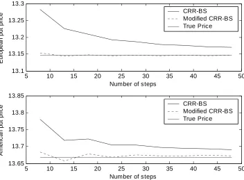
distribution, as is the case for the unmodified lattice schemes. Figure 1 displays the improvement
obtained with the modified CRR binomial tree for European and American put options. For the
European option, the modified CRR approach yields much smaller price biases with respect to the
analytic solution, than the unmodified CRR approach. In the American case, the biases are also
improved by the modification, though the improvement is more moderate. Note that all lattice
approaches in this paper, whether with or without our modification, are implemented with the
Broadie and Detemple (1996) idea of using Black-Scholes prices at the penultimate time step.
Technically, the modification is implemented by replacing the expectations under the risk neutral
probability measure, by an equivalent expression under an alternative probability measure. This
equivalent expression is specified by the Radon-Nikodym derivative. The family of alternative
probability measures considered here is characterized by a unique parameter that corresponds to
the drift term of the stock price process. A one-dimensional numerical search yields the parameter
that minimizes the price discrepancy. Since this minimization can be performed with trees of very
small dimension (say, 10 or 20 time steps), the additional work is typically very small in respect of
the precision gain.
The approach is generic in the sense that it can be adapted to the most lattice schemes available
in the literature. Examples treated here are the CRR and Jarrow-Rudd binomial trees, Kamrad and
Ritchken’s trinomial tree, and the trinomial equivalent of the explicit difference, p.d.e. approach.
The paper is divided as follows. After this introduction, Section 2 presents background concepts
on the changes of measures considered in this study. We next show in Section 3 how to apply
these measure changes in order to modify existing lattice schemes. Section 4 contains the details
regarding the numerical implementation and the results of our numerical study.
2
Background
Under the assumption of complete and arbitrage free markets, Harisson and Kreps (1979) have
shown the existence of a unique risk neutral probability measureQ which allows the computation
the price of a European option, under a constant risk free rate assumption, can be written as :
V0 = EQ £
e−rTf(ST, K) ¤
(1)
whereST is the stock price at timeT,the maturity date of the option, Kis the strike price,r is the
constant risk free rate and f(ST, K) = max [φ(ST −K),0] with φ= 1 for call options and -1 for
put options is the payofffunction of the option. For an American style option, the situation is more
complex because of the early exercise possibility. It can however still be written as an expected
value:
V0 = sup
τ
EQ£e−rτf(ST, K) ¤
(2)
where the supremum is over all stopping times τ ≤T.
This way of expressing the expected values in the option price formula is not unique. Indeed, it is
well known that, through Radon-Nikodym theorem (see Baxter and Rennie 1996), the expectation
under one probability measure Q can be expressed as an expectation under another equivalent
probability measureQ∗. For example, for the European option case, the price could be written as
V0 = EQ ∗·
e−rTf(ST, K)
dQ dQ∗
¸
(3)
where dQdQ∗ is the Radon-Nikodym derivative. Theoretically, both expressions lead to identical prices.
However, in practice, since these expectations must often be assessed numerically, equation (1) and
(3) may obtain different estimated values. For example, in the Monte Carlo simulation context, the
estimated price obtained under the alternative measure may have a different variance that the one
obtained with the risk-neutral measure. This is the rational for the importance sampling approach
which is commonly encountered in the Monte Carlo simulation literature.
In order to compute option prices using an alternative measure such as the one given by equation
(3), an expression for the Radon-Nikodym derivative must be available. One way to obtain such
an expression is through the stochastic process specified for the underlying security. In the
Black-Scholes context, the dynamics of the stock price under the risk neutral measureQ is specified as
with S0 = s0 and W is a standard Brownian motion under the risk neutral measure Q. To keep
the problem tractable, we restrict the change of measure considered here to the class of measures
©
Qλ :λ∈Rª preserving the geometric Brownian motion structure of the stock price. Indeed, as shown in Appendix A, the new dynamics for the stock price underQλ is
dStλ=λStλ dt+σStλ dWtλ, (5a)
withS0λ =s0 and the Radon-Nikodym derivative, in this particular case, expressed as a likelihood
ratio dQdQλ =L
¡
STλ,λ¢where
L³STλ,λ´= exp
·
r−λ σ2 ln
µ
STλ s0
+1
2(λ−r)
r+λ−σ2 σ2 T
¸
. (6)
Equipped with these expressions for the likelihood ratio and the dynamics of the stock price, it is
now possible to compute theoretically and/or numerically expectations under alternative probability
measures. In the next section, we see how these formula can be applied to modify existing lattice
approaches such as binomial or trinomial trees for example.
3
Implementing change of measures to lattice approaches
Consider a lattice with n time steps of length T /n. The stock price at time iTn (i= 0,1, ..., n) at
thejth node of the lattice is denoted bysi,j. The probability, under the risk neutral measureQ, of
reaching node si+1,k from node si,j is represented byqi,j→k. A lattice scheme simply specifies how
the prices and probabilities can be computed given the length of the time step, the initial stock
price, the interest rate and the volatility parameter. These specifications are usually obtained by
imposing the equality between thefirst two moments of the approximate and target distribution.
To adapt a lattice to the alternative probability measureQλ, it suffices to note that the change
of measure from Q to Qλ preserves the geometric Brownian motion structure of the stock price. The difference is the drift coefficient which is no longer r butλ. It is therefore straightforward to determine the stock prices and the transition probabilities of theQλ−lattice by replacingr byλin the design for si,j and qi,j→k. We will therefore define sλi,j as the stock price at the ith time step
In the original Q−lattice, European and American option prices can be obtained by working
backward from the end of grid. Indeed, using the familiar dynamic programming principle, the
option value at theith time step and the jth node is
vi,j = max (
φ(si,j−K), e−r
T n
X
k
vi+1,kqi,j→k )
, i < n (7a)
with vn,j = max{φ(sn,j−K),0}.Unfortunately, a well known draw back of lattices such as the
binomial or trinomial tree is the jagged convergence pattern exhibited by the computed price. We
will therefore adopt here a simple modification proposed in Broadie and Detemple (1995) which
considerably smooths out the convergence pattern. The modified algorithm directly starts the
computations at time stepn−1 and computes the Black-Scholes price instead of the continuation
valuevn−1,j i.e.
vi,j = max (
φ(si,j−K), e−r
T n
X
k
vi+1,kqi,j→k )
, i < n−1 (8a)
withvn−1,j=BS ¡
sn,j;r,σ, K,Tn ¢
denoting the Black-Scholes price for a European style option with
initial stock pricesn,j, strike priceK, time to maturity Tn, risk free rater and volatility coefficient
σ.
Using this general framework, it is straightforward to adapt the algorithm for the Qλ−lattice. Indeed, the discretized equivalent for the likelihood ratio (6) simply becomes
li,j(λ) = exp "
r−λ σ2 ln
Ã
sλi,j s0
!
+1
2(λ−r)
r+λ−σ2 σ2 i
T n
#
(9)
and the option values will be computed with
vi,jλ = max
(
φ³sλi,j−K´ln,j(λ), e−r
T n
X
k
vλi+1,kqλi,j→k
)
, i < n−1. (10a)
with vλn−1,j =BS³sλn−1,j;r,σ, K,Tn´ln−1,j(λ). Note that for the American case, since the prices
in the tree are those with respect to Qλ, it is important to multiply the early exercise value with the likelihood ratio in the dynamic programming equation. Working backward to the tree will lead
to an estimate of the option price. Appendix B shows how specific lattice schemes such as CRR
In practice, the value of λ must be assessed numerically. The idea is to build a lattice with a small number of time steps and use a numerical procedure to find a value λ∗ which achieves a target objective. For example, the value ofλ could be set by minimizing the discrepancy between the estimated European option pricev0λ∗ and the Black and Scholes formulaBS(s0;r,σ, K, T). As
shown in the next section, this value of λ∗ might not be unique and, interestingly, a given value of λ∗ is not sensible the number of time steps. In other words, a value of λ working well for 10 time steps will also work well for 20 or more time steps. This suggests the use of an alternative
objective function. One could, for example, compute prices of American options with two lattices
using n1 and n2 time steps (n1 = 10 and n2 = 20 for example) and choose a λ minimizing the
distance between the two computed prices. These ideas will be examined in the section presenting
the result of numerical experiments.
4
Numerical results
4.1
A detailed example
This section provides a simple numerical example using the CRR (1979) lattice with a Black-Scholes
price at the penultimate time step (CRR-BS hereafter). This example will provide some intuition
on how the expected values and probability distributions are altered under the alternative measure.
The following parameter values are used: s0 = 100, r= 0.05,σ= 0.4, T = 1 and n= 3.With these
and the formulas for the CRR (1979) lattice given in Appendix B we haveu= 1.2597, d= 0.7937,
qλ=r = 0.4785 and qλ=λ∗ = 0.6042 for λ∗ = 0.218. This last value was found using a numerical search algorithm minimizing the distance between the price obtained with theQλ−CRR-BS lattice with 10 time steps and a Black-Scholes price.
Since in this framework the stock prices remain identical under all measures, it is instructive to
compute the discrete distribution at time step n−1 for the stock price using λ=r andλ= 0.218 that is the value ofλ which as been identified numerically to provide accurate prices. Using these distributions, it is then possible to make helpful comparisons showing how the proposed modification
the initial stock price inn−1 steps can be written as:
χλj = (n−1)! j! (n−1−j)!
³
qλ´j³1−qλ´n−1−j×ln−1,j(λ).
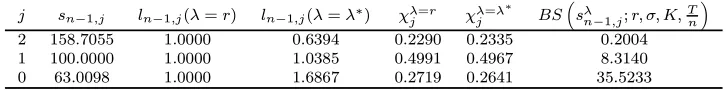
Table 1 reports the computed probabilities χλj=r and χλj=λ∗ with the associated option prices at step n−1. From the numbers in this table it is easy to see that the expected value and standard
deviation (discounted) are 100 and 32.2560 when computed with χλ=r
j while they are 99.98 and
32.2696 when computed with the distribution χλ=λ∗
j . The European put option price computed
with both measures are, respectively, 13.3989 and 13.1151 while the Black-Scholes price is 13.1459.
This shows that the discrete distribution that was originally built to exactly match the first and
second moments of the target distribution is modestly altered in order to remove the large bias in
terms of price from the original CRR-BS approach. This alteration of the probability distribution
has a very small effect on the discounted expected stock price. Indeed, the changes in probability
for large stock prices are compensated by the changes in probabilities for low stock prices. However,
this is not the case when computing the expected value of the put option payoff which has a low
sensitivity to the probability changes associated to large stock prices and a high sensitivity to the
changes associated with low stock prices.
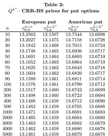
Table 2 examines the computed American put option prices as the number of time step is
increased using both the CRR-BS binomial tree andQλ∗—CRR-BS binomial tree. These numbers can be compared to benchmark values obtained from the Black-Scholes formula for the European
put and a 15000 step CRR-BS binomial tree for the American put. As it can be seen, the option
prices computed with 20 or 30 steps Qλ∗—CRR-BS lattice are more accurate than those obtained with 100 time steps with the CRR-BS lattice.
The results presented in this table are of course specific to the chosen example. Furthermore,
the additional work required by the algorithm is not taken into account. We will therefore present
in the next subsections a numerical study that will assess the performance of the algorithm in terms
of computer time and precision for a large test pool of option contracts.
4.2
The optimization algorithm
4.3
Numerical study
In order to obtain a more general assessment on the quality of the method, we perform an analysis
similar to Broadie and Detemple (1996). The analysis begins by choosing a large test pool of options
using randomly selected parameter values based on pre-determined distributions. For each option,
the prices using the Q−lattice and the Qλ∗−lattice are computed and compared to a benchmark value. We keep track of the computation times and the pricing errors.
The following distributions are used for the parameter values, with each parameter value drawn
independently of the others: φequals 1 or−1 with probability 1/2 for each value,T is distributed uniformly between 0.1 and 1.0 year with a probability of 0.75, and uniformly between 1.0 and
3.0 years with a probability of 0.25; S0 = 100 and K is uniform between 70 and 130; r is, with
probability 0.8, uniform between 0 and 0.1, and with probability 0.2, equal to 0 andσ is uniformly distributed between (0,1; 0.6).
Using the simulated parameter values, the lattice prices and the benchmarks are computed
and compared. We use the root mean square error as our measure of aggregate pricing error.
Specifically,
RM S(m) =
v u u t1
m
m X
i=1
e2
i, (11)
whereei =|Ci(lattice)−Ci|/Ci;Ci is the benchmark obtained for theith option; andCi(lattice) is
theith price obtained with the Q−lattice or theQλ−lattice. The variable mstands for the size of the test pool. In our comparison study, we usem= 1 000 and eliminate the cases whereCi <0.50
to avoid large relative errors caused by a small divider.
To be continued ....
A
Radon-Nikodym derivative
Define
Wtλ =Wt− λ−r
σ tfor anyt≥0 (12)
and note that the replacement ofWtbyWtλ+λ−σrtin Equation (4) leads to Equation (5). We would
like that the distribution ofWλ
Wt isN(λ−σrt, t) under the measureQλ. SinceWtisN(0, t) under measureQandN(λ−σrt, t) under
the measureQλ, the change of measure is expressed as a ratio of density functions :
L(Wt,λ) =
1 √
2πtexp h
−12 W2 t t i 1 √
2πtexp ·
−12
(Wt−λ−σrt)
2
t
¸ = exp
Ã
−λ−r
σ Wt+
1 2
µ λ−r
σ ¶2
t
!
. (13)
By a simple change of variable, the likelihood ratio is expressed as a function of theQλ−Brownian motion :
L³WTλ,λ´= exp
"
−λ−r
σ W λ T − 1 2 µ λ−r
σ ¶2 T # . (14) Finally, since
STλ =s0exp ·µ
λ− σ 2
2
T +σWTλ
¸
(15)
implies that
WTλ = ln
³Sλ
T
s0
´
−
³ λ−σ22
´
T
σ , (16)
the likelihood ratio can also expressed as a function of the stock price under Qλ:
L
³
STλ,λ ´
= exp
−λ−r σ
ln
³Sλ
T
s0
´
−
³ λ− σ22
´ T σ − 1 2 µλ −r σ ¶2 T = exp ·
r−λ σ2 ln
µ
STλ s0
+1
2(λ−r)
r+λ−σ2 σ2 T
¸
.
B
Lattice scheme under alternative measures
B.1
Binomial trees
Many binomial trees are designed on similar basis. The stock price at ith time step and the jth
node is
si,j =s0ujdi−j, i∈{0,1, ..., n}, j ∈{0,1, ..., i} (17)
where u and d are the multiplicative constants for up and down movements in the tree. The
probability, under the risk neutral measureQ, of an upward move isq, i.e.
qi,j→k=
q ifk=j+ 1
1−q ifk=j 0 otherwise.
To choose the different constants u, d and q, many authors proposed to match the two first
moments of the binomial stock price with those of the target continuous time stochastic process
which lead to the two following equations related respectively to the expectation and the variance:
qu+ (1−q) =erTn (19a)
qu2+ (1−q)d2−e2rTn =e2r T n
³
eσ2Tn −1
´
. (19b)
Because there is three variables and two equations, there is some freedom to assess a value to one
of the variable. This lead to the different versions of the binomial tree.
B.1.1 Cox, Ross and Rubinstein
In the binomial tree proposed by Cox, Ross and Rubinstein (1979), we have
u= exp
" σ r T n #
andd= exp
" −σ r T n # . (20) and
q= exp
£
rTn¤−d
u−d =
exp£rTn¤−exp
· −σ q T n ¸ exp · σ q T n ¸ −exp · −σ q T n ¸ (21)
To adapt this tree to the measure Qλ, note that the stock price remains the same
sλi,j =s0ujdi−j =s0exp "
(2j−i)σ r
T n
#
(22)
since it does not depends onr. The probabilityqλ of an upward move becomes
qλ= exp
£
λTn¤−d
u−d =
exp£λTn¤−exp
· −σ q T n ¸ exp · σ q T n ¸ −exp · −σ q T n
¸. (23)
The likelihood ratio for the ith time step and thejth node is
li,j(λ) = exp "
r−λ
σ (2j−i) r
T n +
1
2(λ−r)
λ+r−σ2 σ2 i
T n
#
B.1.2 Jarrow and Rudd
In the binomial tree proposed by Jarrow and Rudd (1983), the constants are
u= exp
"µ
r−σ
2
2
T n +σ
r
T n
#
,d= exp
"µ
r−σ
2
2
T n −σ
r
T n
#
andq = 1
2. (25)
To adapt this binomial tree under the measure Qλ, it suffices to modify the multiplicative
constants which are now given by :
uλ = exp
"µ λ− σ
2
2
T n +σ
r
T n
#
and dλ = exp
"µ λ−σ
2
2
T n −σ
r
T n
#
. (26)
The transition probabilities remains the same because there are not function of r. The likelihood
ratio becomes
li,j(λ) = exp "
−λ−σ r
r
T
n(2j−i)− 1 2
µ λ−r
σ ¶2 iT n # . (27)
B.2
Trinomial trees
B.2.1 Kamrad and Ritchken
The trinomial tree proposed by Kamrad and Ritchken (1991) match the two first moments of the
stock return to their theoritical value. In this particular set up, the stock price at ith time step
and thejth node is
si,j =s0exp "
(i−j)σ r 3 2 r T n #
, i∈{0,1, ..., n}, j ∈{0,1, ...,2i} (28)
The transition probabilities, under the risk neutral measureQ, are
qi,j→k= 1 3 + 1 3σ ³
r−σ22´ qTn ifk=j+ 1
1
3 ifk=j
1 3 −
1 3σ
³
r−σ22´ qTn ifk=j−1
0 otherwise.
To adapt this tree to the change of measure, note that the stock price remains the samesλi,j =si,j
since it does not depends onr. The transition probabilities becomes
qi,jλ →k=
1 3+ 1 3σ ³
λ−σ22´ qTn if k=j+ 1
1
3 if k=j
1 3−
1 3σ
³ λ−σ22
´ q T
n if k=j−1
0 otherwise.
(30)
The likelihood ratio for the ith time step and thejth node is
li,j(λ) = exp "
r−λ
σ α(i−j) r
T n +
1
2(λ−r)
r+λ−σ2 σ2 i
T n
#
. (31)
B.2.2 The explicitfinite difference approach
It can be shown that he explicitfinite difference method is equivalent to the trinomial tree approach.
The stock price atith time step and thejth node is
si,j=s0+ (j−i)∆s, i∈{0,1, ..., n}, j ∈{0,1, ...,2i} (32)
where ∆s is the distance between two consecutive stock price. The transition probabilities, under
the risk neutral measureQ, are
qi,j→k= 1 2 ¡
σ2j2−rj¢T
n if k=j+ 1
1−σ2j2Tn if k=j
1 2
¡
σ2j2+rj¢Tn if k=j−1
0 otherwise.
(33)
To adapt this tree to the change of measure, note that the stock price remains the samesλi,j =si,j
since it does not depends onr. The transition probabilities becomes
qi,j→k= 1 2 ¡
σ2j2−λj¢Tn ifk=j+ 1 1−σ2j2Tn ifk=j
1 2
¡
σ2j2+λj¢Tn ifk=j−1
0 otherwise.
(34)
The likelihood ratio for the ith time step and thejth node is
li,j(λ) = exp ·
r−λ σ2 ln
µ
s0+ (j−i)∆s
s0
+ 1
2(λ−r)
r+λ−σ2 σ2 i
T n
¸
B.3
The Markov chain
The Markov chain method has one distinct feature. Unlike the traditional lattice and finite
dif-ference methods, the Markov chain approach allows one to de-couple the partitioning of time and
state. In other words, one can use time steps suitable for a particular contingent claim without
be-ing unduly constrained to have a particular set of state values. This feature proves to be extremely
useful when early exercise or path dependency in present and/or when the postulated underlying
price dynamic is a discrete-time stochastic process. This design feature provides three useful
oper-ational properties. First, the approach yields a simple recursive matrix formula for valuing options
(European, American and exotic). Second, the transition probability matrix associated with the
Markov chain is highly sparse, which makes it possible to significantly reduce storage requirement
and computation time with the use of sparse matrix techniques. Third, the method can be easily
adapted to different theoretical models.
We refer to Duan and Simonato (2001) for a full description of the method. The adaptation of
the state space and the transition matrix to the model under the alternative probability measure
Qλ is straight forward. This change of measure allows to reduce the dimension of the state space without affecting the number of exercise dates, a feature that is not possible using the trees. This
is particularly important in the pricing of American option since too few exercise dates result in
an underpricing of the option.
To be continued ...
C
References
References
[1] Baxter, M. and A. Rennie, 1996,Financial Calculus, Cambridge University Press.
[2] Broadie, M. and J. Detemple, 1996, American Option Valuation: New Bounds, Approximations, and a Comparison of Existing Methods, Review of Financial Studies 9, 1211-1250.
[3] Cox, J, S. Ross and M. Rubinstein, 1979, Option Pricing, A Simplified Approach, Journal of Financial Economics 7, 229-264.
[5] Duan, J.C., Gauthier, G. and J.G. Simonato, 2003, A Markov Chain Method for Pricing Con-tingent Claims,Stochastic Modeling and Optimization, edited by D. D. Yao, H. Zhang et X.Y. Zhou, Springer, 333-362
[6] Figlewski, S. et B. Gao, 1999, The adaptive Mesh Model: a New Approach to Efficient Option Pricing, Journal of Financial Economics 53, 313-351.
[7] Hull, J.C. and A. White, 198, The Use of the Control Variate Technique in Option Pricing, Journal of Financial and Quantitative analysis 23, 237-251.
[8] Jarrow, R. A. and A. Rudd, 1983, Option Pricing, Richard D. Irwing, Homewood.
[9] Kamrad, B. and P Ritchken, 1991, Multinomial Approximating Models for Options withkState Variables, Management Science 37, 1640-1652.
[10] Tian, Y., 1993, A modified Lattice Approach to Option Pricing, Journal of Futures Markets 13, 563-577.
Table 1: Probability distributions under alternative measures
j sn−1,j ln−1,j(λ=r) ln−1,j(λ=λ∗) χλ=j r χλ=λ
∗
j BS
³ sλ
n−1,j;r,σ, K,
T n
´
2 158.7055 1.0000 0.6394 0.2290 0.2335 0.2004 1 100.0000 1.0000 1.0385 0.4991 0.4967 8.3140 0 63.0098 1.0000 1.6867 0.2719 0.2641 35.5233
sn−1,j is the stock price at time stepn−1 in statej; ln−1,j(λ) is the likelihood ratio at time stepn−1 in statej; χλj is
the probability of reaching statejinn−1 steps from the initial stock price;BS³sλ
n−1,j;r,σ, K,
T n
´
Table 2:
Qλ∗—CRR-BS prices for put options
European put American put
n vλ=0,0r vλ=λ
∗
0,0 vλ=0,0r vλ=λ
∗
0,0
10 13.2563 13.1507 13.7544 13.6698 20 13.2027 13.1475 13.7158 13.6728 30 13.1842 13.1468 13.7015 13.6724 40 13.1748 13.1465 13.6936 13.6717 50 13.1691 13.1464 13.6893 13.6719 60 13.1652 13.1463 13.6864 13.6719 70 13.1625 13.1462 13.6843 13.6718 80 13.1604 13.1462 13.6826 13.6717 90 13.1588 13.1461 13.6811 13.6714 100 13.1576 13.1461 13.6799 13.6712 200 13.1517 13.1460 13.6742 13.6699 300 13.1498 13.1460 13.6723 13.6694 400 13.1488 13.1459 13.6712 13.6690 500 13.1482 13.1459 13.6705 13.6688 1000 13.1471 13.1459 13.6691 13.6683 2000 13.1465 13.1459 13.6684 13.6680 3000 13.1463 13.1459 13.6682 13.6679 4000 13.1462 13.1459 13.6680 13.6678 5000 13.1461 13.1459 13.6679 13.6678
vλ=r
0,0 is the option price computed with the original CRR-BS lattice whilevλ=λ
∗
0,0 is the option price computed with the
Qλ∗— CRR-BS lattice. The benchmark values for the European and American put options are 13.1459 and 13.6677 and are
obtained with the Black Scholes formula and a 15,000 step CRR-BS lattice. Parameter values: s0= 100, K= 100, r= 0.05,σ=
5 10 15 20 25 30 35 40 45 50 13.1
13.15 13.2 13.25 13.3
Number of steps
E
u
rope
an put
pri
c
e CRR-BS
Modified CRR-BS True Price
5 10 15 20 25 30 35 40 45 50
13.65 13.7 13.75 13.8 13.85
Number of steps
A
m
e
ri
c
an
pu
t p
ri
c
e CRR-BS
[image:18.612.120.472.219.478.2]Modified CRR-BS True Price