Modification of conductivity due to acceleration of the ionospheric medium

© European Geosciences Union 2008

Geophysicae

Modification of conductivity due to acceleration of the

ionospheric medium

V. V. Denisenko1,2, H. K. Biernat3, A. V. Mezentsev1, V. A. Shaidurov1, and S. S. Zamay1

1_{Institute of Computational Modelling, Russian Academy of Sciences, Siberian Branch, Krasnoyarsk, 660036, Russia} 2_{Siberian Federal University, Krasnoyarsk, 660041, Russia}

3_{Space Research Institute, Austrian Academy of Sciences, Schmiedlstrasse 6, 8042 Graz, Austria}

Received: 23 February 2006 – Revised: 16 April 2008 – Accepted: 16 May 2008 – Published: 31 July 2008

Abstract. A quantitative division of the ionosphere into dy-namo and motor regions is performed on the base of empiri-cal models of space distributions of ionospheric parameters. Pedersen and Hall conductivities are modified to represent an impact of acceleration of the medium because of Amp´ere’s force. It is shown that the currents in theF2layer are greatly reduced for processes of a few hours duration. This reduc-tion is in particular important for the night-side low-latitude ionosphere. The International Reference Ionosphere model is used to analyze the effect quantitatively. This model gives a second high conducting layer in the night-side low-latitude ionosphere that reduces the electric field and equatorial elec-trojets, but intensifies night-side currents during the short-term events. These currents occupy regions which are much wider than those of equatorial electrojets.

It is demonstrated that the parameterσd=σP+σH6H/6P that involves the integral Pedersen and Hall conductances

6P,6H ought to be used instead of the local Cowling con-ductivityσCin calculations of the electric current density in the equatorial ionosphere. We may note that Gurevich et al. (1976) derived a parameter similar toσd for more general conditions as those which we discuss in this paper; a more detailed description of this point is given in Sect. 6. Both,

σdandσC, appear when a magnetic field line is near a non-conducting domain which means zero current through the boundary of this domain. The main difference betweenσd andσC is thatσd definition includes the possibility for the electric current to flow along a magnetic field line in order to close all currents which go to this line from neighboring ones. The local Cowling conductivityσCcorresponds to the current closure at each point of a magnetic field line. It is adequate only for a magnetic field line with constant local conductivity at the whole line when field-aligned currents do not exist because of symmetry, butσC=σdin this case. So, Correspondence to: H. K. Biernat

([email protected])

there is no reason to use the local Cowling conductivity while the Cowling conductance6C=6P+62_H/6P is a useful and well defined parameter.

Keywords. Ionosphere (Electric fields and currents; Equa-torial ionosphere; Modeling and forecasting)

1 Introduction

The ionosphere is usually considered as a conductor with a given conductivity distribution when global electric fields and currents are simulated. Considering the high conductiv-ity in the direction of the magnetic field, a two-dimensional approach is appropriate. The magnetic field lines are equipo-tentials and the ionospheric conductor may be represented by Pedersen and Hall conductances which are equal to integrals along magnetic field lines of the corresponding local conduc-tivitiesσP, σH (Gurevich et al., 1976).

If the conductor is moving, then Ohm’s law is valid in the moving frame of reference. An additional term appears in the laboratory frame of reference that is proportional to the velocity. This kind of electric field generator is subject of the dynamo theory. The motion of the medium is mainly defined by neutral winds and it is slightly disturbed by the Amp´ere force in the E-region of the ionosphere since the density is large there. So, this conductor moves in the magnetic field and works as a magnetohydrodynamic generator. In contrast to the E-region, the medium in the F-region is guided by the Amp´ere force that corresponds to a division of the ionosphere into dynamo and motor regions (Hargreaves, 1979).

It is always difficult to estimate a common result of many factors when they exist altogether. So, we use a simplified way to analyze the factors separately. Such an approach may be insufficient for nonlinear systems when few factors are strong, but it is useful as a step in research. A pressure gra-dient is taken into account in the frame of a local model (Maeda, 1977). A complicated model like this of Namgal-adze et al. (2000) is necessary to analyze all forces which define the motion in the ionosphere.

The motion of the medium may be approximately taken into account as a modification of the conductivity. The con-cept of defining some effective conductivity which represents a moving conducting medium is not new. It is done by Aka-sofu and Chapman (1972) under the assumption of a steady-state motion. It takes different time to accelerate electrons, ions, and neutrals up to a steady-state motion. The conduc-tivity dependence of the electric field on the frequency is an-alyzed by Vanyan et al. (1973) in the case when neutrals are almost at rest. The model (Akasofu and Dewitt, 1965) repre-sents a modification of the Pedersen conductivity for an elec-tric field which is harmonic in time. Our approach differs mainly in that an unsteady process is regarded as a relaxation to a new steady state after a moment when the electric field is changed. We add an analysis of integrated conductivities which is important for models of large scale electric fields.

In this paper, we analyze only local effects. A global prob-lem aught be solved with this modified conductivity to find a more realistic electric field. Such a problem is described in Sect. 5.

2 The conductor motion

Let us consider a homogeneous conductor which moves in magnetic B and electric E fields. Let us split the vectors E into field-aligned componentsEkparallel to the magnetic field and the normal components E⊥. The Ohm law is valid in the rest frame of reference,

jk=σkEk, (1)

j⊥=σPE0⊥−σH[E0⊥×B]/B, (2)

E0⊥=E⊥+ [u⊥×B], (3)

where j is the current density, quantitiesσP, σH, σkare the Pedersen, Hall, and field-aligned conductivities and u is the conductor velocity. We use SI units. In the case of our inter-est, the electric field and velocity are normal to the magnetic field.

Since we analyze separately the motion of the conducting medium, whose appearance is due to the electric and mag-netic fields, no force but the Amp´ere one needs be taken into account in the equation of motion

ρ du⊥

dt = [j⊥×B], (4)

whereρis the mass density.

We define right-handed Cartesian coordinates with the x-and z-axes along E⊥and B, and put the y-axis to complete the triad.

The solution for the problem (2–4) with zero velocity at the momentt=0 is given by the following formula,

ux

uy

=

0

−u0

+u0e−t /τ

sin(t /T )

cos(t /T )

, uz=0, (5) where u0=[E⊥×B]/B2is the drift velocity,u0=|u0|, and the parametersτ andT are

τ =ρ/(B2σP), T =ρ/(B2σH). (6) In the(ux, uy)plane this solution is presented by a spiral. It starts at the zero point and goes to the point(0,−u0)which corresponds to the drift. The direction of this spiral rotation is defined by the sign ofσH. LetσH>0 for definiteness.

As a consequence of the Eqs. (2, 3, 5), the current density varies with time,

j⊥=(σPcos(t /T )+σHsin(t /T )) e−t /τ E⊥−

−(−σPsin(t /T )+σHcos(t /T )) e−t /τ [E⊥×B]/B. By analogy with the law (Eq. 2), this equality may be inter-preted as an Ohm’s law in the laboratory frame of reference with the following time varying values of the conductivity tensor components,

σP(t )

σH(t )

=e−t /τ

cos(t /T ) sin(t /T ) −sin(t /T )cos(t /T )

σP

σH

. (7) If the process under analysis covers timet0, it is natural to de-fine an average value of the conductivity. Time integration of the formula (7) and rearrangement withτ/T=σH/σP gives

< σP >=σP

τ t0

(1−exp(−t0/τ )), (8)

< σH >=σH

T t0

sint0

T

exp(−t0/τ ). (9) Whent0τ, T, the average values are equal to the original ones. For long-term processest0τ, T, the average conduc-tivities<σP>and<σH>go to zero. As it is shown in the next sections, the typical situation in the Earth’s ionosphere isTt0. This permits to simplify Eq. (9),

< σH >'σH exp(−t0/τ ). (10) Then, only thet0/τ ratio defines<σP>and<σH> modi-fication. The average Hall conductivity<σH>decreases as the exponent of the duration of the processt0. The average Pedersen conductivity<σP>varies twice less than<σH> does, whent0is small, and decreases as 1/t0, whent0τ. Anyway, the conductivities vanish because of the conductor acceleration if the process is long enough.

3 Empirical model of the main ionospheric parameters

Our calculations are based on the following empirical mod-els: The International Reference 2001 (IRI), the Mass Spec-trometer Incoherent Scatter 1990 E (MSISE), the Interna-tional Geomagnetic Reference Field 1945-2010 (IGRF-10). We used Fortran software of these models from the web page of NASA’s Space Physics Data Facility (NASA, 2006).

The concentration of the main ions O+,O+₂,NO+, and electrons, as well as their temperatures, we define by IRI. To include the height region of 80–100 km we choose the model (Danilov and Smirnova, 1995) among those included to IRI. All other alternatives inside IRI are solved as a choice of standard versions. The main neutral gases N2,O2,O con-centrations, we define by the MSISE model (Hedin, 1991). Above 120 km this model does not differ from MSIS (Hedin et al., 1977).

The model IRI demonstrates the convergence of electron, ions and neutrals temperatures, when the height decreases to 120 km. This permits one to define a common temperature. We use the MSISE model to define the temperature below 120 km because it can not be done by IRI.

The collision rates of the electrons can be calculated by the following formulae (Banks, 1966)

ν(e,O2)=1.82×10−16n(O2)(1+0.036 p

Te) p

Te,

ν(e,N2)=2.33×10−17n(N2)(1−0.000121Te)Te,

ν(e,0)=2.8×10−16n(O)pTe,

νei =54×10−6neTe−1.5,

νe =νei+ν(e,O2)+ν(e,N2)+ν(e,0), (11) wheren(O2)is the concentration of the molecules O2etc.,

ne andTe are the density and Kelvin temperature of elec-trons, andνeis the total electron collision rate. For the ions – neutrals collisions, we use the formulae (Stubbe, 1968)

ν(O+)=1.86×10−15 _T

i +Tn 2000

0.37 n(O)+ +10−15n(O2)+1.08×10−15n(N2),

ν(O2+)=1.17×10−15 _T

i +Tn 2000

0.28

n(O2)+

+0.75×10−15n(O)+0.89×10−15n(N2), ν(NO+)=0.83×10−15n(O2)+

+0.76×10−15n(0)+0.90×10−15n(N2). (12) The parameters given by the IRI model and Eqs. (11, 12) are sufficient to calculate the components of the conductiv-ity tensor by the following formulae (see, e.g. Hargreaves, 1979),

σk=e2N 1

meνe

+X

i 1

miνi !

,

σP =e2N

νe

me(ω2e+νe2)

+X

i

νi

mi(ω2_i +ν_i2) !

,

σH =e2N

ωe

me(ω2e+νe2)

−X

i

ωi

mi(ω_i2+ν_i2)

, (13)

whereωeandωi are the electron and ions gyrofrequencies,

meandmiare their masses. The summation is over the main ions O+,O+₂,NO+,i=1,2,3.

4 Typical acceleration periods

The above presented set of models permits us to calculate spatial distributions of ionospheric parameters for any date and time. Equations (6) give the values of the parametersτ

andT which represent the period of a conductor acceleration, which is also the period of the conductivity relaxation to the zero value.

For definiteness we choose a moment of universal time when there is midnight at the Northern geomagnetic pole on the 90-th day of a year that corresponds to the Spring equinox. Other conditions are the following: low geomag-netic activity, theApindex equals 4, moderate Solar activity, the Covington index equals 130.

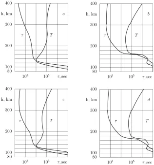
The vertical cross-sections of τ andT above the points with geomagnetic latitudes θm=90◦, 45◦ and longitudes

ϕm=180◦, ϕm=0◦ are presented in Fig. 1. Hereh is the height from the Earth’s surface. We use these points as typi-cal ones for the low latitude and middle latitude ionosphere. There is midnight at the points withϕm=0◦and midday at the points withϕm=180◦.

TheτandT height distributions moderately vary withθm,

ϕmin the day-side ionosphere. In the height region of 160– 300 km, both parameters are much larger in the middle lat-itude ionosphere than near the equator as it can be seen by comparison of Fig. 1d and b.

A typical time of a quasi-stationary process in the Earth’s ionosphere may be defined ast0=104s because of daily vari-ations.

As it can be seen in Fig. 1, there isT≥104s elsewhere. The value of the factor in the bracket in the expression (9) does not differ much from unity ifT >t0,

1≥ T t0

sint0

T ≥sin 1'0.85, (14)

and it goes to unity whenT increases.

80 100 200 300 400

h, km a

τ T

103 ₁₀5 _τ,sec 80

100 200 300 400

h, km b

τ T

103 ₁₀5 _τ,sec

80 100 200 300 400

h, km c

τ T

103 ₁₀5 _τ,sec 80

100 200 300 400

h, km d

τ T

103 ₁₀5 _τ,sec

Fig. 1. Vertical cross-sections of the time parametersτandT. The panels (a), (b) correspond toθm=90◦, (c), (d) correspond toθm=45◦. The left and right columns present midday and midnight values, respectively.

The parameter τ decreases with height. It equals three hours at the height of about 140 km at midday and at 170– 250 km at midnight. Since the functionsτ (z)monotonously decrease with height for every fixedθm,ϕmthere is a point

z(θm, ϕm)in whichτ=t0. The set of these points taken for all values ofθm, ϕmforms some surface. This surface divides the ionosphere into two regions. The motion of the iono-spheric medium is almost independent of the electric field below the surface. The effective conductivity (8, 9) is cor-respondingly close to the originalσP, σH. This region is re-ferred as the dynamo region (Hargreaves, 1979). Above this surface, the medium is quickly accelerated up to the drift ve-locity and its effective conductivity decreases significantly. Equations (8, 9) estimate such a separation quantitatively. It depends on the typical period of the process under consider-ation,t0.

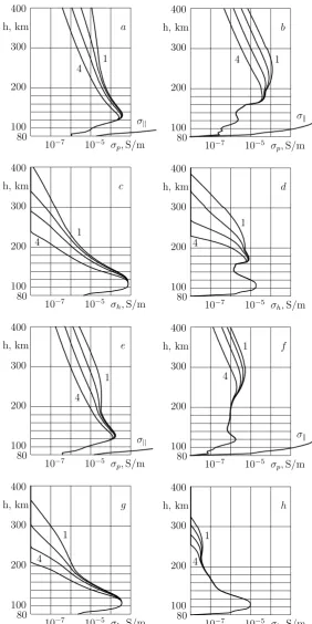
The curves 1 in Fig. 2 show the height distributions of

σP, σH for the same conditions as Fig. 1, respectively. The panels (a), (c), (e), (g) are plotted for midday and the pan-els (b), (d), (f), (h) present midnight distributions. Curves 2, 3, 4 show the effective conductivities<σP>, <σH>(Eqs. 8,

9) which are calculated for the processes witht0=1/3,1,3 h, respectively.

Height distributions ofσkare partially plotted at the same panels asσP to demonstrate thatσkis thousands times larger thanσP above 100 km.

The effective Pedersen conductivity is smaller than the original σP by a factor of ten above 300 km. However, its decrease by a factor of two in the region of the maximum value is more important for two-dimensional models of the ionospheric conductor.

The effective Hall conductivity <σH> decreases much more in comparison toσH than<σP>does in comparison toσP. It occurs above 200 km where even the originalσH is small.

Figure 2b, d, f, h shows that the effective conductivities during night time are also significantly less than their original values whent0is large enough.

80 100 200 300 400

h, km a

1 4

10−7 ₁₀−5 _σ p,S/m

σ

80 100 200 300 400

h, km b

1 4

10−7 ₁₀−5 _σ p,S/m

σ

80 100 200 300 400

h, km c

1 4

10−7 ₁₀−5 _σ

h,S/m 80 100 200 300 400

h, km d

1 4

10−7 ₁₀−5 _σ h,S/m

80 100 200 300 400

h, km e

1 4

10−7 ₁₀−5 _σ p,S/m

σ

80 100 200 300 400

h, km 1 f

4

10−7 ₁₀−5 _σ p,S/m

σ

80 100 200 300 400

h, km g

1

4

10−7 ₁₀−5 _σ

h,S/m 80 100 200 300 400

h, km h

1

4

10−7 ₁₀−5 _σ h,S/m

5 2-D model of the ionospherical global conductor

Considering the high conductivity in the direction of the magnetic field, a two-dimensional approach is appropriate. The magnetic field lines are equipotentials and the iono-spheric conductor may be represented by Pedersen and Hall conductances which are equal to integrals of the correspond-ing local conductivitiesσP, σH (Hargreaves, 1979). We fol-low the approach by Gurevich et al. (1976) where this proce-dure is made accurately from the mathematical point of view by introducing some base surface that crosses all magnetic field lines and it is used both, for numbering of the field lines and as a fictitious 2-D conductor film that is equivalent to a real space distributed conductor.

Here we present a simplified version of the approach by Gurevich et al. (1976). Such a simplification is possible when magnetic field is normal to the base surface. For a potential magnetic field B=−grad8.Any surface8=const may be used as such a base surface since the vector grad8is always normal to the surface8=const. We use the empirical model IGRF that represents just the potential part of the geomag-netic field. It would be impossible if it includes maggeomag-netic perturbations created by the currents in the magnetosphere. An additional simplification is possible since we use semi geodetic coordinates on the base surface. Since the surface

8=const is smooth such a coordinate system exists (Korn and Korn, 1968).

The conductivity is a scalar in the atmosphere below 80 km and it is a tensor with theσP,σH,σkcomponents in the iono-sphere which can be calculated by Eq. (13).

Let us suppose that the conductor does not move. Then the Ohm law (Eq. 1) stays for the parallel components and the law (2) is simplified for the normal ones,

j⊥=

σP −σH

σH σP

E⊥. (15)

In Fig. 2 it is demonstrated how the difference betweenσk andσP increases in the height region 80–100 km. Sinceσk in the ionosphere is thousands times larger thanσP,σH it is possible to idealize this inequality as

σk= ∞. (16)

The conductivities σP, σH are small below 80 km and can not make a substantial contribution to the integrals. More-over, the two-dimensional approximation fails there because the field-aligned conductivityσkbecomes comparable toσP. The approximation σk=∞ is satisfactory above 80 km, if electric fields above 100 km are under analysis (Stening, 1985). If electric fields and currents below 100 km are of interest, it would be necessary to solve another conductiv-ity problem in some domain below the new boundary about 100 km taking obtained potential distribution at this bound-ary.

The equality (16) means that the electric current along a magnetic field line can be arbitrary while the electric field componentEkequals zero,

Ek=0. (17)

Since E=−grad V , the electric potential V is constant at each magnetic field line as a result of the identity (17) and

E⊥= −grad⊥V . (18)

In such a model, a magnetic field line is an object with its own value of the electric potentialV. It can obtain or loose charge by currents j⊥ and it does not matter for its total charge in what point of the magnetic field line j⊥exists be-cause charge can go free along this line according to Eq. (16). Denote the semi geodetic coordinates at the base surface as m, h. Then the distance between two points at the base surface which are close to each other equals

g2(1m)2+(1h)2, (19)

where the components of the metric tensor are g2,1. The procedure of such a coordinate system construction is pre-sented in (Korn and Korn, 1968). The third coordinatelis the arc length along the magnetic field line from the point at the base surface.

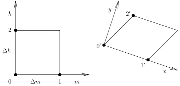
In purpose to define the conductance for a magnetic field line let us analyze a thin magnetic field tube that has a square cross-section in some plane normal to the magnetic field. The cross-section is shown in Fig. 3 with thel axis directed out of the paper. We put magnetic field lines from the point 0 till some point 00_{. We construct local Cartesian coordinates} near the point 00_{with the z-axis along magnetic field. We put} the x-axis from the point 00 _{to point 0}0 _{in that the field line} from the point 1 intersects the planez=0. We put the y-axis to complete the triad. We also design the magnetic field line from the point 2 till it crosses the planez=0 in some point 20.

Since we analyze a thin magnetic field tube with small

g1m=1hwe get some parallelogram in the plane z=0 as the projection along magnetic field lines of the quadrangle into the planel=0. This is shown by the right-hand panel in Fig. 3. We denote the coordinates of the points 10, 20as

(1x1,0,0), (1x2, 1y2,0), (20) with zero point 00coordinates by construction.

Because of the expression (18), the potential differences between the points 1,0 and between 2,0 are equal to

1V1= −Emg1m, 1V2= −Eh1h (21) and between the points 10,00and between 20,00

u u u

u

u u

0 Δm 1 m

Δh h 2 0 1 2 x y

Fig. 3. Normal cross-sections of a magnetic field tube which starts at them, hplane. The right panel presents another cross-section of the same tube. The local Cartesian coordinatesx, y, zare introduced near the point 00.

The potential differences1V1, 1V2(Eq. 21) are the same as1V₁0, 1V₂0 (Eq. 22) because the values of the potential at the points 0 and 00_{, 1 and 1}0_{, 2 and 2}0_{are equal since these} pairs belong to the same field lines. This permits to calculate the electric field in the planez=0 from the last formulae,

Ex Ey =   g1m 1x1

0

−

1y21x1

1h 1y2   Em Eh . (23)

This electric field E⊥produces the current j⊥by Ohm’s law (Eq. 15), jx jy =

σP −σH

σH σP

Ex

Ey

. (24)

Let us consider a prism 0<z<1z and currents 1I1, 1I2 through two of its sides which have height1zand contain the edges 0010and 0020, correspondingly. We must multiply the normal components of current density (Eq. 24) with the squares of these rectangle sides,

1I2 1I1 =1z

1y2−1x2 0 1x1

jx

jy

. (25)

The same currents through the sides of the analyzed magnetic tube may be provided by some surface current density1J at a fictitious thin conducting film in the plane l=0 if the components1Jm, 1Jhof1J are such that

1I2=1Jm1h, 1I1=1Jhg1m. (26) Taking into account Eqs. (23–26), we can express

1Jm 1Jh =1z 1y2 1h

−

0

g1m !

σP −σH

σH σP × ×   g1m 1x1

0

−

1y21x1

1h 1y2   Em Eh . (27)

This means that the conducting prism 0<z<1zcan be re-placed by a fictitious conducting film in the planel=0 with

conductance tensor16 that is the coefficient in front of the vector(Em, Eh)in Eq. (27)

16=1z  

1x₂2+1y₂2

1x11y2

σ

−

1x2

1y2

σ

−

σ

−

1y2

σ

+

σ

1x1

1y2

σ



, (28) where the equalityg1m=1his used.

By summation of the incomes from all cross-sections of the magnetic field tube, we obtain the conductance of such a film in the planel=0 which, in respect of currents exchange between magnetic field lines, is equivalent to the surrounding of the whole magnetic field line. The resulting Ohm law can be written as J=6E, or in detailed form as

Jm

Jh

=

6

6

6

6

E

E

. (29)

Since the coordinatelis the length along this magnetic field line it can be used as a local Cartesian coordinatedl=dznear the planez=0. After integration of Eq. (28), we get

6= Z

 

1x₂2+1y2₂

1x11y2

σ

−

1x2

1y2

σ

−

σ

−

1y2

σ

+

σ

1x1

1y2

σ



dl. (30) We see that only ratios of 1x1, 1x2, 1y2 are present and they are known functions oflbecause the magnetic field lines are proposed to be known as well as theσP, σH space distri-butions.

If the magnetic field lines are parallel straight lines, then

1y2/1x1=1, 1x2=0. (31)

Therefore Eq. (30) is simplified to

6= Z

σP −σH

σH σP

dl, (32)

what permits to write down the tensor6as

6=

6P −6H

6H 6P

θm

70o

90o

110o

0o ₉₀o ₁₈₀o ₂₇₀o _ϕ

m 360o

Fig. 4. Geomagnetic equator with segments of the magnetic field lines which start and finish at the height of 80 km, and cross the geomagnetic

equator at the height of 400 km. A possible base surface near the geomagnetic equator is plotted by the thin line.

with Pedersen and Hall conductances 6P, 6H which are obtained from the local Pedersen and Hall conductivities

σP, σHintegrated along a magnetic field line. If a segment of the magnetic field line with nonzeroσP, σHis short enough, then the equalities (31) are approximately valid for any mag-netic field. This is so in the high and middle latitude iono-sphere where the magnetic field lines cross the ionospheric conducting layer with some angle ξ from the vertical that increase the length as1l=1H /cosξ,where1His the ver-tical size of the layer.

It is necessary to emphasize that such a tensor6with only

6P, 6H components stays only in coordinatesm, hnormal to the magnetic field.

Since the parameters of the ionosphere do not vary much in the horizontal direction, the integrals (32) can be calcu-lated as height integrals in high latitudes and just height in-tegrals are often referred as to integral conductivities (Harg-reaves, 1979), but there is no reason to do so in low latitudes since the electric field is constant not with height but along magnetic field lines which are almost horizontal.

We use the IGRF model for the geomagnetic field. Fig-ure 4 presents the position of the geomagnetic equator at the height 400 km and a possible base surface at the same height. They are presented by thick and thin lines, respectively. The abscissa is the geomagnetic longitudeϕmand the ordinate is the geomagnetic colatitudeθm. Both lines vary with height because of the non-dipolar part of the geomagnetic field, but, the variations are hardly seen in the figure for heights of 80– 400 km. The segments of the magnetic field lines are also plotted. These lines cross the geomagnetic equator at the height of 400 km. The ends of the segments lie at a height of 80 km.

The geomagnetic equator is the line of the horizontal netic field and the base surface has constant value of the mag-netic potential. We mention that the magmag-netic field is not nor-mal to the geomagnetic equator in nondipolar models and the base surface is defined so that the magnetic field is normal to it. Any equipotential surface may be used as the base surface. Here we have chosen the surface that gives the best values in the following estimations.

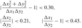
We have calculated the magnetic field lines in the neigh-borhood of the lines presented in Fig. 4 that permitted us to obtain the values of the geometrical coefficients in the inte-gral (30) and to find that they satisfy the inequalities

|1x

2 2+1y

2 2

1x11y2

−1|<0.30, |1x2

1y2

|<0.21, |1x1 1y2

−1|<0.43. (34)

The lines which start below these lines and finish at the same height of 80 km satisfy these inequalities as well. The seg-ments of the field lines which are in the height interval 80– 400 km in the rest ionosphere also satisfy these inequalities if the base surface is normal to the lines and because of that the line segments are shorter than the lengths of those shown in Fig. 4 and the non–dipolar components of the geomagnetic field are not too large. But similar geometrical coefficients additionally appear if we take into account that the Northern and Southern semi-lines must be united by the same poten-tial value at least in low and middle latitudes. It is shown by Denisenko and Zamay (1992) how to construct such a base surface for the whole ionosphere as a set of small sheets and to transform it into a unit circle for a dipolar magnetic field. For the real geomagnetic field this can be done only numeri-cally.

The numbers in the inequalities (34) estimate the error if the expression (30) is simplified with Eq. (32). If we use only the dipolar component of the geomagnetic field, then the base surface and the equator become the planeθm=π/2 and the calculations give

1x₂2+1y₂2 1x11y2

−1' −0.06, 1x2

1y2

'0.00, 1x1 1y2

−1'0.07. (35)

The shape of a dipolar magnetic field line is known to be

r=r0sin2θ, ϕ=ϕ0, (36)

wherer0, ϕ0are the coordinates of the point in the equatorial plane andr, θ, ϕare the coordinates of any point at this field line. So, the coefficients can be calculated analytically,

1x₂2+1y₂2 1x11y2

= √ 1

1+3 cos2_θ,

1x2

1y2

=0, 1x1 1y2

For the lines in the height interval 80–400 km, Eq. (36) gives

|π/2−θ|<13◦_{and the values given by Eq. (37) correspond} to the numerically obtained ones in the equalities (35).

As it is shown by the estimations (34, 35), the simpli-fied definition of the conductances (32) is rather precise for a dipolar field, and it gives an error up to 40% for the real field. Nevertheless, for simplicity, we use just Pedersen and Hall conductances6P, 6H near the geomagnetic equator in our further demonstrations of the results of the plasma ac-celeration, because the effect under analysis decreases the conductivity a few times.

The current density (Eq. 24) satisfies the local charge con-servation law

div j= ∂jx ∂x +

∂jy

∂y + ∂jz

∂z =q, (38)

where nonzeroq appears if some given extrinsic current jex exists. Then

q= −div jex. (39)

For example such an extrinsic current appears in accordance with Ohm’s law (Eq. 2)

jex=

σP −σH

σH σP

[u×B], (40)

when the velocity u in the ionosphere is given. Such a cur-rent source is under analysis in the dynamo theory (Akasofu and Chapman, 1972). Different given currents in the magne-tospheric parts of the magnetic field lines also may be taken into account as jex.

The integral of the local Eq. (38) over the magnetic field tube presented in Fig. 3 fromlsttilllfinis equal to the sum of the currents through its four sides whose cross-sections are presented in Fig. 3 plus currents through the ends. In accordance with the definition of the fictitious current at the base surface, the sum of these four currents is equal to

I

[(Jm, Jh)×(dm, dh)]. (41) The current through the end of the magnetic field tube is

jk1x11y2, (42)

where the field-aligned current densityjkand the square of the tube1x11y2are taken atlstor atlfin. If we regard the whole tube that starts below the ionosphere and finishes also below the ionosphere in the opposite hemisphere, thenjk=0 at the both ends. Otherwisejk at one end of the tube may be nonzero as some given current from the magnetosphere to the ionosphere.

The integral of the right-hand side of Eq. (38) is Z lf in

lst

q1x11y2dl. (43)

Let us divide the terms (41–43) by the square of the tube at the base surface g1m1h and make the limit 1m→0,

1h→0. We obtain a 2-D operator of the divergence of the integral (41) that in accordance with (Korn and Korn, 1968) is

Div J= 1 g

_∂

∂m(Jm)+ ∂ ∂h(gJh)

, (44)

and the function

Q= Z lfin

lst

qdx1dy2 g1m1hdl−jk

dx1dy2

g1m1h lfin

lst

(45) as the difference between the terms (43) and (42). If the an-alyzed part of the magnetic field tube is short enough, then the fractions in this expression is equal to unit.

The total result of this integration of the local Eq. (38),

Div J=Q, (46)

is the charge conservation law for the fictitious current at the base surface.

The Eqs. (46, 18, 29) give the model of the introduced fictitious conducting film,

−Div(6GradV )=Q, (47)

where the operator Grad produces them, hcomponents of the full vector gradV.

The sharp decrease of the conductance below the iono-sphere may be idealized as a jump to zero at some height

h1. Then,h=h1 is the boundary with insulator that means zero normal component of the current density,

Jh|h=h1 =0. (48)

If we approximately putσP=σH=0 ath<h1while integra-tion in Eq. (30), then6→0, whenh→h1. This happens be-cause the length of the segment of the magnetic field line that is inside the layer withσ6=0 goes to zero when the top of the field line goes to the boundary of this layer. Such a singular-ity6→0 is a bad feature for Eq. (47). To avoid this singular-ity, we need conductivitiesσP, σH in some region belowh1 that makes it possible to calculate nonzero conductance6at

h≥h1.

It is possible to takeh1about 80 km in the daytime iono-sphere andh1about 90 km in the nighttime ionosphere. Less values of h1 meet two difficulties. As it can be seen in Fig. 2a, b, quantityσk is not much larger thanσP, σH be-low these heights and so the 2-D model can not be used. The second problem is due to the restrictions of the IRI model. It gives the electron density above 65 km in the daytime iono-sphere and only above 80 km in the nighttime ionoiono-sphere. In the next section, it is demonstrated that these heights include the main part of the ionospheric conductor.

In purpose to plot the conductance6 distributions at the common heightsh>80 km, we extrapolate the electron den-sity below 80 km in the night time ionosphere as

where the parametersn0_e, h0are defined by thene values at

h=80 km andh=85 km at every vertical line. The Eq. (49) permits to represent a sharp decrease of the values6P, 6H belowh=80 km without their jumps to zero ath=80 km, that would be if we were to putne=0 and henceσP=σH=0 be-lowh=80 km.

The Eq. (47) must be completed by the boundary condi-tion (48) and some condicondi-tions for other boundaries. In the dipolar magnetic field with zero electric potential difference between adjoint points in the Northern and Southern Hemi-spheres the base surface can be chosen as the planeθm=90◦ and the cylindrical coordinatesr, ϕcan be used ash, mwith metricalg=rin Eq. (19). Then condition (48) becomes

−6rr

∂ V ∂ r −6rϕ

1

r ∂ V ∂ ϕ

r=RE+h1

=0, (50)

and the condition, that means absence of a singularity near the magnetic poles,

V|_r→∞=0, (51)

completes the model.

Equation (47) takes the shape

−1 r

∂ ∂ r

r6rr

∂ V ∂ r +6rϕ

∂ V ∂ ϕ

−

−1 r

∂ ∂ ϕ

6ϕr

∂ V ∂ r +6ϕϕ

1

r ∂ V

∂ ϕ

=Q, (52)

with the tensor6calculated by Eq. (30).

If the parts of the magnetic field lines are regarded sepa-rately for the Northern and Southern Hemispheres, thenQ

includes given field-aligned currents above the ionosphere in accordance with Eq. (45). The boundary value problem be-comes more complicated in such a model (Denisenko, 2002) in comparison to Eqs. (50–52).

6 Cowling conductance

The Cowling conductance

6C =6P +6H2/6P, (53)

is widely used (Forbes, 1981) in theories of equatorial elec-trojets. It appears in the models of the boundary layer for the problem defined by Eqs. (46, 18, 29, 48).

As usual, an approximate model of the boundary layer is based on its small width in comparison to typical distance along the boundary. The ratio of these scales is regarded as to be a small parameter,ε. In our case,ε=δh/δmsince the boundary (48) is the lineh=h1. Let us now denoteh2as theh coordinate of the line, that separates the boundary layer from the main part of the conductor. These lines may be curved in general case, but, here we simplify the procedure (Gurevich et al., 1976) to make it more visual. We neglect the differ-ence of the metric coefficients from Eq. (31). We also neglect

the curvature of the Earth’s surface and suppose that the base surface is a plane. Then, semi geodetic coordinatesm, hmay be chosen as Cartesian ones with a vertical directionhand a horizontal directionmalong the geomagnetic equator (Korn and Korn, 1968). The metric tensor becomes a unit one in such a case, what means thatg=1 in Eq. (19). As usual, we don’t take into account the charge source inside the bound-ary layer, which meansQ=0 in the charge conservation law (Eq. 46).

After these simplifications, Eq. (46) takes shape

∂Jm

∂m + ∂Jh

∂h =0. (54)

In order to compare the scales of Jm, Jh, let us inte-grate this equation over the quadrangle h1<h<h1+δh,

m1<m<m1+δm, where the sideh=h1belongs to the bound-ary with insulator (48) andm=m1is an arbitrary point at the boundary. After integration by parts,

Rh1+δh

h1 Jm(m1+δm, h) dh−

Rh1+δh

h1 Jm(m1, h) dh+ +Rm1+δm

m1 Jh(m, h1+δh) dm=0, (55)

where the integral over the sideh=h1is omitted because it equals zero in view of Eq. (48). Since each integral of a con-tinuous function over a segment equals the length of the seg-ment multiplied by the value of this function in some point inside the segment, this equation may be rewritten and re-solved as

Jh(m∗, h1+δh)=

= δh

δm(Jm(m1+δm, h

∗∗

)−Jm(m1, h∗∗∗)), (56) where∗marks some point inside proper segment.

Since we are interested in a large scale processes when the distanceδmof a remarkableJmchange is much larger than

δh, the ratio in the right-hand side is a small parameterε. The first order boundary layer approximation corresponds to the idealization of this small parameter, asε=0, meaning

Jh(m∗, h1+δh)=0. (57)

Since the values of coordinates m∗, h1+δh describe any point, the vertical component of the current density equals zero inside the boundary layer,

Jh=0. (58)

Similar analysis of the equation

∂Eh

∂m − ∂Em

∂h =0, (59)

which is equivalent to Eq. (18) in our Cartesian coordinates, shows that the horizontal component of the electric field is independent of the highthinside the boundary layer,

Since the conductance tensor in the Ohm’s law (29) has the shape (33) in our simplified case, we can write Eq. (29) as

Jm

Jh

=

6

−

6

6

6

!

E

E

. (61)

In combination with Eqs. (58, 60) this means

Jm(m, h)=6PEm(m)−6HEh(m, h)

0=6HEm(m)+6PEh(m, h). (62) From the second equation we obtain

Eh(m, h)= −(6H/6P)Em(m), (63) and, resolving the first one, we obtain the main formula of the boundary layer

Jm(m, h)=(6P +6H2/6P)Em(m). (64) The coefficient is referred to as the Cowling conduc-tance (53). It relates the components of the current density and electric field which both are normal to the magnetic field and parallel to the boundary. They are along the geomagnetic equator.

SinceEmis independent ofh, it is simple to integrate ex-pression (64) over the heighthto get the total current in the boundary layer,

I (m)= Z h2

h1

Jm(m, h) dh= Z h2

h1

6Cdh

Em(m)=

=A(m)Em(m), (65)

where the total conductance of the boundary layer is a func-tion of the coordinatemalong the boundary and is denoted asA(m).

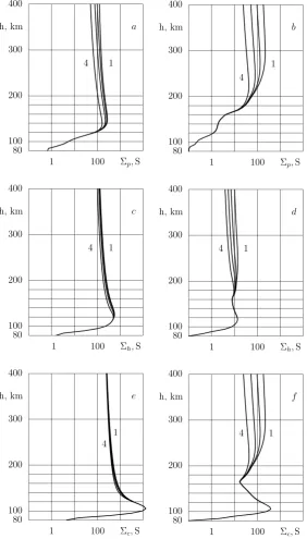
Such a boundary layer approach is correct but of no sense if6C in the vicinity of the boundary is of the same order of magnitude as inside the main part of the conductor. Some small currentI (m)is separated in this strip, but it does not help to analyze the global problem. This is not the case in the ionosphere of the Earth and this boundary layer is observed as the equatorial electrojet. Typical distributions of6Cabove the geomagnetic equator are presented in Fig. 5e, f. Large values of6Care seen in theδh≈50 km layer in the midday. This layer is much wider at midnight. Its upper boundary is not shown because the6C decrease to about 10 S middle latitude value is rather slow. If we are interested in the total currents in the equatorial electrojets, the integration (65) can be done tillh=150 km at midday. The night time structure is analyzed in Sect. 8.

If the problem given by Eqs. (46, 18, 29, 48) is solved numerically, the sharp variations of the coefficients inh di-rection produce difficulties. They can be avoided by separat-ing the boundary layer takseparat-ingh=300 km to make6P, 6H smooth functions in the rest domain. The Cowling conduc-tance6Citself is not used there. The boundary layer approx-imation is correct in this case, sinceh2−h1≈200 km is much

less then a few thousands kilometers distance along the equa-tor, indeed. Its adequateness looks problematic ifh2−h1 ex-ceeds 1000 km, but it is not necessary to use a boundary layer approximation for such a wide region.

There are experimental estimations of the width of this boundary layer, which means the vertical size above the geomagnetic equator. The longitudinal component of the electric field is constant for about 400 km in the vicinity of the geomagnetic equator (Forbes, 1981) that corresponds to Eq. (60). This means that at least one of the two nontrivial base features for the 2-D boundary layer theory (58), (60) is adequate in theEandF regions of the ionosphere above the geomagnetic equator. This leads to the Cowling conductance

6C and then toσd. Nevertheless, only test calculations with

different choice of its upper boundary can show the error. The total current (Eq. 65) in the strip h1<h<h2 varies along the equator. If we cut a part frommtillm+δm, the charge conservation law (Eq. 55) for this part takes the shape

I (m+δm)−I (m)+ Z m+δm

m

Jh(m, h2) dm=0. (66) Let us divide this equation byδmand go to the limitδm→0, then

∂I (m)

∂m +Jh(m, h2)=0. (67)

Using the denotation of Eq. (65), we obtain

∂

∂m(A(m)Em(m))+Jh(m, h2)=0. (68)

This is the boundary condition that must be used at the new boundaryh=h2which excludes the boundary layer from the global problem. The second order boundary layer approxi-mation (67) improves the first order approxiapproxi-mation (58). Ap-proximations of the next orders are not really used.

When the solution of the 2-D problem is obtained, the electric field at the new boundaryEm(m)can be used to cal-culate inside the boundary layer the electric field and current by Eqs. (60, 63, 58, 64). Also the 3-D current density may be calculated by Ohm’s law (24), wherex is along the equator as it ism. So, the horizontal current density in the equatorial electrojet equals

jx =σPEm(m)−σHEh(m, h)=

=(σP +σH6H/6P)Em(m). (69)

The coefficient in the last expression

σd=σP +σH6H/6P, (70)

is equal to the local Cowling conductivityσC=σP+σ_H2/σP, if the ionosphere is a homogeneous layer orσH/σP=const at each magnetic field line. Then Eq. (32) gives

6H/6P=σH/σP. The real space distribution ofσP, σH do not satisfy any of these conditions. The difference between

80 100 200 300 400

h, km a

1 4

1 100 Σp,S

80 100 200 300 400

h, km b

1 4

1 100 Σp,S

80 100 200 300 400

h, km c

1 4

1 100 Σh,S

80 100 200 300 400

h, km d

1 4

1 100 Σh,S

80 100 200 300 400

h, km e

1 4

1 100 Σc,S

80 100 200 300 400

h, km f

1 4

1 100 Σc,S

Fig. 5. Conductances6P,6H,6C above the geomagnetic equator (curves 1). The left and right columns present midday and midnight values, respectively. Curves 2, 3, 4 are for effective conductances fort0=1/3,1,3 h.

Integration of this parameterσdalong a magnetic field line is simple since6P, 6H are constants for this line

Z

σddl= Z

σP dl+(6H/6P) Z

σHdl=

=6P +6H2/6P =6C. (71)

So, the Cowling conductance 6C is not equal to the inte-gral of the local Cowling conductivity as it is sometimes

done instead of using the Pedersen and Hall conductances and Eq. (53).

7 Modification of the ionospheric conductance

In Sect. 5, the conductances6P, 6H are defined for a mag-netic field line. We identify a field line by the height h

100 200 300 h, km

400

a

log Σ 3

2

1

0

100 200 300 h, km

400

b

log Σ

4

3

2

1

0o ₉₀o ₁₈₀o ₂₇₀o _ϕ

m 360o

100 200 300 h, km

400

c

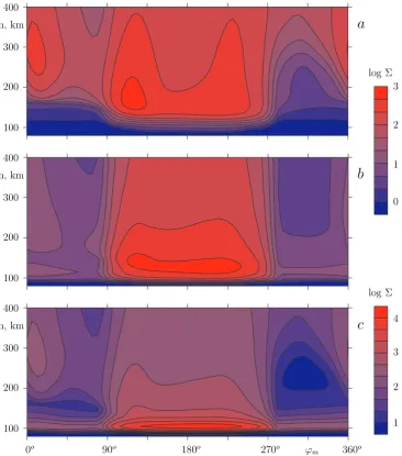
Fig. 6. Conductance distributions at the base surface near the geomagnetic equator for a short-term process. Panel (a) is for log₁₀(6P), panel (b) is for log₁₀(6H), panel (c) is for log10(6C), where conductances inSunits are used. The abscissa is the geomagnetic longitude ϕmand the ordinatezis the height at which the magnetic field line crosses the base surface. The top color scale is for6P, 6H. The bottom color scale is for6_C. The values at the neighbor plotted contours differ 3

√

10'2 times. The contours6_P<1S, 6_H<1Sand6_C<10Sare not plotted and a common color is used for these small values of6.

coordinates. The conductances6P, 6H as functions of h are shown in Fig. 5a, b and 5c, d, respectively. The left column presents midday values above the point with geo-magnetic coordinates θm=90◦, ϕm=0◦. The right column presents midnight that is at the point with geomagnetic co-ordinatesθm=90◦, ϕm=180◦at a taken moment of universal time.

Figure 5e, f present the midday and midnight Cowling conductance6C, as it is defined in Sect. 6.

The curves 1–4 in Fig. 5 have the same meaning as those in Fig. 2. The curves marked with number 1 present the orig-inal6P,6H,6C and the curves 2, 3, 4 correspond to the

processes witht0=1/3,1,3 h. As it is seen in Fig. 5a, c, e, the main modification in the day-side ionosphere is the6P modification. Fort0=3 h, quantity 6P decreases twice as compared to a short-term process. All three conductances de-crease significantly in the night-side ionosphere. The effect under consideration, in fact, cancels the second conducting layer, the conductance of which for the short-term processes is larger than the conductance of the layer below 160 km. Since the Pedersen conductance below 160 km is small, its 30 times decrease above 200 km is very important.

100 200 300 h, km 400

a

b

log Σ

2

1

0 100

200 300 h, km 400

c

d

100 200 300 h, km 400

−90o ₀o _ϕ

m 90o

e

−90o ₀o _ϕ

m 90o

f

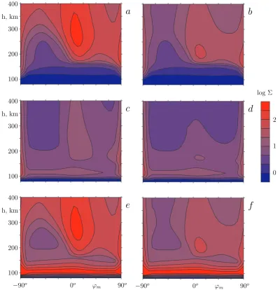
Fig. 7. Conductance distributions above the night half of the geomagnetic equator. Left panels show conductances for a short-term process.

Right panels show conductances for a long-term process, for which modifications of the conductivities are done fort0=3 h. Panels (a), (b) are for log10(6P), panels (c), (d) are for log10(6H), panels (e), (f) are for log10(6C), where conductances inSunits are used. The color scale is common for all panels. A common color is used for6<1Sand the contours6<1Sare not plotted.

the geomagnetic equator are presented. The abscissa is the geomagnetic longitudeϕm and the ordinate is the height at which the magnetic field line crosses the base surface, that is shown in Fig. 4. A few magnetic field lines which cross the base surface at the height of 400 km are plotted in Fig. 4. They correspond to the proper points at the upper boundary 400 km in every panel of Fig. 6. At the contours plotted in Fig. 6, the conductances have constant values. We use a log-arithmic scale for the conductances in units of Siemens. The values of6to neighboring contours differ 3

√

10 times which is approximately twice. The color scales as well as values at the contours are shown in the right panel. A special color scale is used for6C since it has maximal values higher than

6P,6H. For the purpose to present the main features of the

6 distributions, detailed color and contour scales are used. They do not permit to present adequately the sharp decrease of the conductances belowh=100 km. So, the color is not varied there as well as some contours are omitted.

Figure 7 shows that the conductances decrease one order of magnitude above 180 km in the whole night-side low-latitude ionosphere for 3 h long processes as compared to the short-term ones. This is also shown for the midnight in Fig. 5.

The main result of the analyzed acceleration is that for the long-term processes, the night-side height distributions of the conductances become similar to the day-side ones with 30 times less scale, as it takes place in the middle-latitude iono-sphere. This is precisely the property which is used practi-cally in all models of the low-latitude ionospheric conduc-tance. Figures 5–7 show that this is wrong for the short-term processes, but indeed, the analyzed acceleration of the medium permits to ignore the conductance of the higher layer for the long-term processes.

8 On the night-side equatorial electrojets

The distributions of the Cowling conductance which are pre-sented in Figs. 6c and 7e, f permit to analyze possible struc-ture of low-latitude electric current systems.

The coefficients of the two-dimensional conductivity equation in coordinateshand the arc length along the base surface are close to6P, 6H as it is show above in Sect. 5. By comparison with these preferential coordinates, a very stretched scale is used in Figs. 6, 7, because the height in-terval of 320 km is much less than the length of the equa-tor. Therefore, the presented region of high conductance is to be identified as a narrow strip along the boundary of the conducting domain. The lineh1=80 km may be taken as an impenetrable boundary.

The total current in the region that includes the magnetic field lines with tops are at the heightsh,h1<h<h2I (m)can be calculated as the integral (65).

If we neglect the difference between the base surface and

θ=90◦plane, then the coordinatemis proportional toϕmand

I (m)is the current along the equator produced by the electric field in the same direction.

As it is seen in Fig. 6c, quantity6C has a sharp maxi-mum at 100–110 km and is large in the height interval 90 km

<h<130 km. Therefore, the electric current is large just in this region above the equator. It is identified as the day-side equatorial electrojet. An additional view of the electrojet in the plane which is normal to thism, h-plane is presented in the end of the section.

The night-side structure is more complicated: One more layer above 200 km is added. The contribution of the F-region to the nighttime current at the equator is known (Takeda and Maeda, 1980). The more detailed scale in Fig. 7f shows that its integral contribution is comparable with the contribution of the layer below 120 km because it is a few times wider. This situation holds for long-term process. For a short-term process, the contribution of this higher layer is one order of magnitude larger than the contribution of the

layer below 150 km as it can be seen in Fig. 7e. Theh co-ordinate in these pictures is the height at which the magnetic field line crosses the geomagnetic equator and it is the maxi-mum height of the line.

The conductances presented in Figs. 6, 7 describe the ficti-tious conducting film that is defined in Sect. 5. Such a model permits to calculate the electric field(Em, Eh)as the solution of the boundary value problem for Eq. (47). The Ohm law (Eq. 29) gives currents at the fictitious film and real space dis-tributed currents are given by the Ohm law (Eq. 24) with the expression (23) for the electric field in the point of interest.

In the analyzed region 80 km<h<400 km near the equa-tor, the Eqs. (60) and (23) mean

Ex

Ey

=

1

−

1y2

−

1x1

1y2

6hm

6hh

! g1m

1x1

Em(m). (72)

The Ohm law (Eq. 24) gives a current which has both, hor-izontal and vertical components, in contrast to the integral current, because the local vertical current at one part of the magnetic field line can be compensated by negative vertical current at another part of the line, so that the total current at the line has a zero vertical componentJh=0.

If we neglect geometrical factors what means no difference betweendx, dy andg dm, dh when the simplified expres-sion (33) is valid, then Eqs. (72) and (24) permit to calculate the current density as

jx

jy

=

σP −σH

σH σP

1

−6H/6P

Ex. (73)

So, the horizontal component of the current density is

jx =σdEx, (74)

and the parameterσ_d is defined by Eq. (70).

It should be mentioned that the remaining z-component of the current density that is field-aligned in this case, can be calculated from the charge conservation law (Eq. 38) after

jx, jyare calculated by Eq. (73).

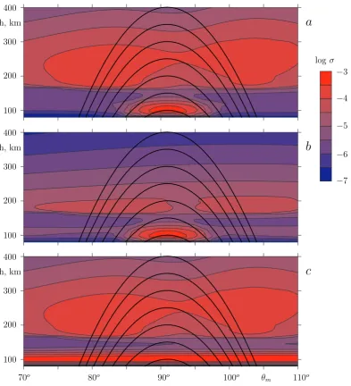
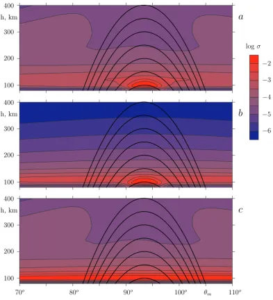
The difference betweenσdand the local Cowling conduc-tivityσCis discussed in Sect. 6. The difference between their values can be seen by comparing Fig. 8a and c for the night time ionosphere, and Fig. 9a and c which present the day time cross-sections of the equatorial ionosphere.

The Cowling conductivity has a maximum value near

h=100 km, because of that, quantityσH has maximum val-ues at the heights 100–120 km and σP is much less there, as it can be seen in Fig. 2. If the whole magnetic field line is situated below 120 km, then the ratio of the integral con-ductances6H/6P is of the same order of magnitude as the maximal value ofσH/σP. Then σd does not differ much fromσCin the points of these lines, which occupy the region

±3◦near the magnetic equator. If a part of the magnetic field line is above 120 km then the integral conductance6P in-creases much in contrast to6H, sinceσP is much larger and

100 200 300 h, km

400

a

log_σ

−3

−4

−5

−6

−7

100 200 300 h, km

400

b

70o ₈₀o ₉₀o ₁₀₀o _θ

m 110o

100 200 300 h, km

400

c

Fig. 8. Conductivity distributions at the surface that consists of the magnetic field lines which cross the geomagnetic equator above the point

ϕm=0. There is midnight in this point. A few magnetic field lines of this sort are plotted. Panel (a) is for log₁₀(σd)for a short-term process, panel (b) is for log₁₀(σd)for a long-term process, panel (c) is for log10(σC)for a short-term process, where conductivities inS/munits are used. The abscissa is the geomagnetic colatitudeθmand the ordinatehis the height. The color scale is common for all panels. The values at the neighbor plotted contours differ

√

10'3.2 times.

120 km. Therefore,6H/6P is much less than the maximal value of σH/σP and maxσdmaxσC at such a magnetic field line. This dramatic difference betweenσdandσCwould not exist ifσP, σHwould have common height distributions. The upper boundary of the region, whereσd can be used is defined by the same restrictions as those for6C, which are mentioned in Sect. 6.

When the local Cowling conductivityσCis used, the limi-tations are stated as “several degrees away from the magnetic equator”. This statement is rather indefinite and a compari-son of Fig. 9a with c shows that the limitation is very sharp.

It is well seen in Fig. 9c that it is hard to cut a proper part from the layer in thatσC is almost homogeneous in the di-rection across the equator. In contrast, we see just the region of the electrojet in theσ_d distributions shown in Fig. 9a and 9b. This region is a sequence of large values of the Cowling conductance6Cfor this group of magnetic field lines.

The integrals Z

jxdh, Z

jzdh (75)

100 200 300 h, km

400

a

logσ

−2

−3

−4

−5

−6

100 200 300 h, km

400

b

70o ₈₀o ₉₀o ₁₀₀o _{θm 110}o

100 200 300 h, km

400

c

Fig. 9. The same as Fig. 8 but near the midday pointϕm=180◦at the geomagnetic equator.

the sphereh=100 km and used for an approximate calcula-tion of the magnetic perturbacalcula-tions below the ionosphere in-stead of being distributed in space current j. So, the vector function (75) is referred to as the equivalent current density.

Since the x-direction is normal to the plane of Fig. 8 and approximatelyEx=const in the domain presented in Fig. 8, these maps also present the current density (74) in the vicin-ity of the geomagnetic equator in A/m units forEx=1 V/m. Figure 9 may be used in the same manner for midday.

Figure 9a shows the concentration of the current in the jet with a horizontal size of about 600 km. This panel is plotted for a short-term process when the ionospheric plasma has zero velocity and the next panel presents the results of plasma acceleration. Figure 9b demonstrates that almost the same jet appears during long-term processes withτ=3 h, but the

modification of the conductivity is valuable outside of the jet.

The conductivity in the F-region is much more important in the nighttime ionosphere. So, the effect of the modifica-tion of the conductivity is stronger. This is demonstrated in Fig. 8a, b. There is a region of a jet and it has about the same size as in the daytime, but there is one more conductor in the F-region that is switched in parallel to the jet region, since they have the sameEx=const. For a short term pro-cess, the parameters of these two conductors are more ob-vious in Fig. 7e since the lineϕm=0 presents just integrals along the magnetic field lines of the conductivityσd(θm, h) as presented in Fig. 8a.

has an about ten times larger integral conductance. So, only about one tenth of the current is below 150 km. It is concen-trated as the equatorial jet in the nighttime ionosphere. The main part of the current occupies the horizontal strip near the equator of about 4000 km width, as it is seen in Fig. 8a. Since this conductor has minimal conductance just above the jet region, the jet hardly can be identified from ground–based measurements of magnetic perturbations.

The conductivityσd for a long-term process with τ=3 h is presented in Fig. 8b. The region of the jet is almost the same as for a short-term process in Fig. 8a, but the second conductor is by about twenty times reduced, what is better seen in Fig. 7f. So, the jet becomes the main conductor and it may be identified by ground based measurements if the total current along the nighttime part of the equatorial ionosphere is strong enough.

It is also important to note that the conductances in the night-side low-latitude ionosphere are much larger than it can be expected if one extrapolates their properties from the middle-latitudes to low latitudes.

We can summarize the results of this section as the expec-tation of essential modifications of the model electric fields and currents in the low-latitude ionosphere compared to the models which use less detailed conductivity models than IRI gives. Our models (Denisenko and Zamay, 1992) are among the latter.

For the long-term processes the modification of the tradi-tional models may be moderate because on one hand the IRI-2001 model gives the second night-side layer of high conduc-tance, and on the other hand, the acceleration of the medium reduces the current in such a layer.

9 Discussion

The reduction of conductivities as obtained in this paper is of the same order as the one in the model by Akasofu and De-witt (1965) which represents the modification of the Peder-sen conductivity for an electric field being harmonic in time (exp(iωt )) in the middle-latitude day time ionosphere. The effective conductivity does not differ much from the steady state conductivity for processes whose duration is much less than one hour. If the time scale of a process is of about few hours, then the conductivity above 200 km decreases by one order of magnitude.

The difference between the conductivities σP, σH and their effective values<σP>,<σH>(Eqs. 8, 9) in the Earth’s ionosphere may be qualified as the reduction or even exclu-sion of conductance in theF2layer forh>200 km for long-term processes.

In addition to the results by Akasofu and Dewitt (1965), we analyzed in detail this effect in the nighttime and low-latitude parts of the ionosphere. It is shown that the reduc-tion of conductivity is more important in the nighttime

iono-sphere, sinceσP is large in theF layer in contrast to the day time ionosphere.

Also, we have calculated the modified values of the con-ductances<6P>,<6H>,<6C>which are necessary for models of large-scale electric fields and currents while the re-search (Akasofu and Dewitt, 1965) was concentrated on the modification of the local conductivitiesσP,σH,σkand their role for the electric field penetration from the ionosphere into the magnetosphere.

We have shown the modification of the conductivities only in some typical conditions in this paper. Real parameters of the ionosphere may be very different. For example, the nighttime F-region has a large variation with solar activity. The midnight conductances6P,6H and6Cat the magnetic field lines, which tops are in the F-region, are presented in Fig. 5b, d, f. They are calculated for a moderate value of Covington Index 130 in this paper. These6P,6H and6C in the F-region can be four times less or twice larger, when Covington Index equals 70 or 190.

Real processes have different variations in time. For a pe-riodical process, the approach (Akasofu and Dewitt, 1965) is better since it is based on functions harmonic in time. If we are interested in some switching from one steady state to another, our approach is more adequate since it describes just a relaxation. One of the advantages of our model for more complicated processes is that<σP>,<σH>are real numbers in contrast to complex values in the model from (Akasofu and Dewitt, 1965). The imaginary parts of that val-ues represent the time delay in the conductivity modification. The parameterτ (Eq. 6) represents the delay in our approach. The proposed modification of the local conductivity ac-cording to Eqs. (8, 9) as well as the model (Akasofu and Dewitt, 1965) is based on the assumption (4) that no force but the Amp´ere one accelerates the medium. The Amp´ere force above the geomagnetic equator may be vertical as well as horizontal. The vertical movement of the ionospheric medium can break pressure balance stronger than the hor-izontal movement. In spite of that, such a motion due to an Eastern or Western electric field is often observed above the geomagnetic equator as the quiet time fountain effect or super-fountain effect during storm times (Tsurutani et al., 2004).

Pressure and friction are supposed to be unchanged in our model. Conversely, the original local conductivitiesσP, σH remain unchanged if the Amp´ere force is negligible. The adequateness of one of these opposite assumptions can be proved only in the frame of a more general model, because of the fact that pressure and other parameters may be changed as a result of the motion. A pressure gradient was taken into account in the frame of a local model by Maeda (1977).

If we have only the simplified model of the ionosphere that is a global conductor with given conductivity and ve-locity distributions, it is useful to calculate the electric fields and currents twice, for givenσP, σHand for effective<σP>,

<σH>. If the results are different, a qualitative analysis of acceleration is needed. In special cases, this examination supports one of the alternatives. For example, a consider-able reduction of the effective conductivity in theF2layer must be always done. In general, a quantitative simulation of the motion is necessary.

Additional questions appear when the model of the iono-spheric conductor (47) is used in the dynamo theory. If the space distribution of the velocity is known, it is possi-ble to calculate the extrinsic current (Eq. 40), its divergence

q (Eq. 39), and the proper term Q(Eq. 45) on the right-hand side of Eq. (47). The modification of the conductivity (Eqs. 8, 9) can not be done in such a case, since the velocity is given. A small time of acceleration in the upper ionosphere that is usually referred to as the motor region means that the velocity of the medium is defined not by the neutral winds but mainly by the electric fields there. It ought be taken into account in the definition of the velocity that may be taken as given only in the dynamo region, where the time of the medium acceleration is large enough. It also should be men-tioned that the components of the velocity not horizontal but normal to the magnetic field are of value.

10 Conclusions

The IRI model gives the second high conductance layer in the night-side low-latitude ionosphere in addition to the main conductor in the E-layer. It reduces the electric field and equatorial electrojets, but intensifies the night-side currents in theF2layer during short-term events. These currents oc-cupy the regions which are much wider than those of the equatorial electrojets.

The local conductivity is to be reduced with Eqs. (8, 9) to take into account the influence of the Amp´ere force. The cor-responding acceleration of the conducting medium reduces the currents in theF2layer. This reduction is maximal in the low-latitude night-side ionosphere.

The presented theory predicts different space distributions of the currents in the night time low-latitude ionosphere dur-ing long-term and short-term events. The long-term currents are expected to be in the E-layer and are concentrated in the electrojet of about the same width as the daytime jet width. During the short-term events the nighttime jet is masked by a much wider current in the F-layer. The electric field above the geomagnetic equator produced by the same volt-age in high latitudes is expected to be much less during the short-term events since the total conductance of the equato-rial ionosphere decreases much because of the medium ac-celeration. This behavior is important for the analysis of the

electric field penetration from the auroral zone till the geo-magnetic equator.

It is demonstrated on the basis of the IRI-2001 model that the parameter (70) σd=σP+σH6H/6P, that involves the Pedersen and Hall conductances6P, 6H of the whole mag-netic field line, define the space distribution of the electric current density in the equatorial ionosphere and the local Cowling conductivityσC=σP+σH2/σP can not be used for this purpose.

Both,σdandσC, appear when a magnetic field line is near a nonconducting domain what means that there is zero cur-rent through the boundary of this domain. Then, the proper component of the current across the magnetic field direc-tion is regarded as to be a small one in some vicinity of this boundary.

The main difference betweenσdandσCis that theσd def-inition includes the possibility for the electric current to flow along a magnetic field line in order to close all currents j⊥ which go to this line from neighboring ones. The local Cowl-ing conductivityσCcorresponds to a j⊥closure at each point of the magnetic field line, which is adequate only if the field-aligned conductivity equals zero or the field-field-aligned current equals zero because of some symmetry. Such a symmetric object is a magnetic field line with constant local conductiv-ity at the whole line and a generator must be also constant if it exists, but thereσC=σd in this case. The first possibility of zero field-aligned conductivity is not appropriate for the ionosphere. So, we see no reason to use local Cowling con-ductivity while the much more adequate parameterσdexists. A similar parameter was introduced long time ago by Gure-vich et al. (1976). This was done in a more complicated form for the more general case in nonorthogonal coordinates. It seems that such a complicated form explains why it is not widely used until now.

The problem of the local Cowling conductivity was dis-cussed by Forbes (1981) in the frame of a 2-D model simi-lar to the model of Gurevich et al. (1976) that we use here. In such a model 6C=6P+6H2/6P. The so called “thin-shell model” which leads toσCwas also analyzed by Forbes (1981). He did not at all reject the usage of “thin-shell model” and properσC, and left it to be used with the rather indefinite restriction “several degrees away from the mag-netic equator”, while, in fact, he did not use such an approx-imation in his model. Here we have performed the next step, which is natural in such an approach, and have changedσC by more general parameterσd.

Acknowledgements. This work is supported by grant 07-05-00135