R E S E A R C H
Open Access
A new joint CTC-attention-based speech
recognition model with multi-level
multi-head attention
Chu-Xiong Qin, Wen-Lin Zhang
*and Dan Qu
Abstract
A method called joint connectionist temporal classification (CTC)-attention-based speech recognition has recently received increasing focus and has achieved impressive performance. A hybrid end-to-end architecture that adds an extra CTC loss to the attention-based model could force extra restrictions on alignments. To explore better the end-to-end models, we propose improvements to the feature extraction and attention mechanism. First, we introduce a joint model trained with nonnegative matrix factorization (NMF)-based high-level features. Then, we put forward a hybrid attention mechanism by incorporating head attentions and calculating attention scores over multi-level outputs. Experiments on TIMIT indicate that the new method achieves state-of-the-art performance with our best model. Experiments on WSJ show that our method exhibits a word error rate (WER) that is only 0.2% worse in absolute value than the best referenced method, which is trained on a much larger dataset, and it beats all present end-to-end methods. Further experiments on LibriSpeech show that our method is also comparable to the state-of-the-art end-to-end system in WER.
Keywords:Speech recognition, End-to-end, Attention mechanism
1 Introduction
Although traditional speech recognition has been devel-oped quite successfully over the past few decades, some of the techniques, including hidden Markov models (HMMs) and Gaussian mixture models (GMMs), require independ-ent hypotheses and extra expert knowledge [1, 2]. Re-cently, end-to-end methods have become able to ignore these burdens and have achieved remarkable results in many speech recognition tasks [3–5]. End-to-end models are usually trained in a data-driven way without much in-sertion of artificial interventions.
As important extensions of end-to-end theory, attention-based models have been successfully applied in speech recognition tasks. Attention-based models are composed of an encoder, a decoder, and an attention layer. The attention layer connects the encoder outputs and decoder outputs. The attention mechanism was first proposed as a machine translation, which does not have too many bounds on alignments. However, it becomes a
many-to-one problem in a monotonic way in speech rec-ognition. Traditional attention types do not have suffi-cient restrictions to keep alignments monotonous or avoid repeated alignments.
Attention mechanisms are always implemented within an encoder-decoder architecture. The attention weights map inputs (with lengthT) to outputs (with lengthL) in speech recognition tasks whereT is much larger thanL. A variety of attentions have been discussed in machine learning tasks and developed into several types in the past few years. They mainly vary in the scoring functions and connection methods.
In the early stage, some attention mechanisms were directly transplanted from other models to speech recognition. Inspired by neural Turing machines (NTM), three attention mechanisms were extended for attention-based speech recognitions. Content-based attention, hybrid attention, and location-based attention generally rely on previous decoder state, previous align-ments, and encoder outputs and only vary in different combinations of them [6,7]. All three attentions are cal-culated using a multi-layer perceptron (MLP). To further
© The Author(s). 2019Open AccessThis article is distributed under the terms of the Creative Commons Attribution 4.0 International License (http://creativecommons.org/licenses/by/4.0/), which permits unrestricted use, distribution, and reproduction in any medium, provided you give appropriate credit to the original author(s) and the source, provide a link to the Creative Commons license, and indicate if changes were made.
* Correspondence:[email protected]
simplify the function, Chan et al. [8] proposed that the final matching MLP be performed with a dot product operation. Using dot product attention together with a pyramidal encoder-decoder model, they obtained state-of-the-art performance in the Google Voice search task.
Although these models used the most common atten-tion types in speech recogniatten-tion, the calculaatten-tions have low bounds to monotonicity, which may generate ran-dom connections between encoders and decoders. We believe current attentions may still be simpler in struc-ture than they should be.
There have been various further research studies aim-ing to adopt better structures for the attention mechan-ism in some specific tasks. For example, Yang et al. proposed the use of word-level attention and sentence-level attention as hierarchical attention networks in document classification [9]. Cui et al. introduced an tention over attention structure where a dot product at-tention is calculated over a dot product of a query and document [10]. Gehring et al. proposed a multi-step at-tention combined with convolutional layers to capture relations among words especially when sentences are long [11]. In speech recognition, a joint CTC-attention architecture was proposed. This model was expected to transfer monotonic alignments from CTC to attention-based part, and it was demonstrated to be quite effective in solving the problem [12,13]. The joint CTC-attention model achieves the best performances in many corpora [14, 15]. However, the joint CTC-attention model does not improve attention mechanisms fundamentally. There are no sufficient modifications in the attention layers.
To address these problems, we propose various im-provements in the attention mechanism. In order to demonstrate the effectiveness of our attention method, we adopt a joint CTC-attention model trained with high-level features. This is a system we have proposed in our previous work [16,17].
Our proposed attention method is described in two parts. First, inspired by [18], we adapt multi-head atten-tions into end-to-end speech recognition so that the model can jointly obtain information from different rep-resentation subspaces at different positions. Second, the outputs of the last two layers in the encoders are utilized to calculate attention scores by multiplying them to-gether. We believe both improvements yield better re-strictions on attentions and therefore provide better accuracy for end-to-end models.
The paper is organized as follows. We first describe the method of the high-level feature-based joint model in Section 2. Section 3 describes our improvements on the attention mechanism using multi-level encoder out-puts and head attentions. We propose a multi-head attention scored with multi-level outputs of an encoder. Section 4 presents experiments using our
improved attention mechanism compared to some typ-ical attention types. Section5concludes our work.
2 Joint CTC-attention model with high-level features
Before introducing our attention method, we first de-scribe a joint CTC-attention model trained with high-level features from our previous work [17]. The high-level features can replace complex convolutional layers. Therefore, this approach reduces the total number of pa-rameters and makes the end-to-end model easier to train. The joint CTC-attention models achieve the best performances among end-to-end models because they are able to transfer restrictions embedded in CTC to at-tention alignments.
2.1 High-level feature extraction
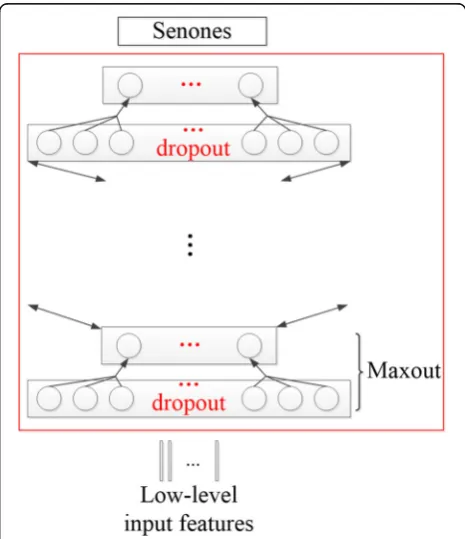
In the high-level feature extraction stage, we use maxout activation with dropout training to avoid the overfitting problem and meanwhile capture better generalities. The schematic structure of the deep neural network (DNN) hidden layers is shown in Fig.1.
DNNs are supervised by tied triphone units that are generated by GMM, while the inputs are classical low-level acoustic features. As analyzed in [16, 17], in order to build a narrow layer to extract high-level features, we apply convex nonnegative matrix factorization (CNMF) to the weight matrix of DNN after training.
As a variant of NMF, CNMF not only has no hard-bound for values, but also restrict the base matrix to convex combinations of columns from the target matrix [19]. Assuming that the target weight matrixXhas a size ofN×M, it is factorized into a base matrixF(with a size of N×R) and a coefficient matrix G (with a size of R× M). We first useK-means to initialize CNMF and obtain cluster indicators H= (h1,…,hk) where K denotes the number of total classes.h1,…,hkare vectors containing
binary values. Then, we initialize G with an empirical setting as we did in the previous research [16,17]:
Gð Þ0 ¼Hþ0:2E; ð1Þ
where E is an identity matrix. F is initialized as cluster centroids:
Fð Þ0 ¼XHD−1
n ð2Þ
Dn= diag(n1,…,nk) and n1, …, nk are the numbers of
each class. CNMF definesFto be linear combinations of columns of X, which isF=XW. According to this con-straint and Eq. (2), we get Wð0Þ¼HD−1
n . Then, G and Ware updated as follows until convergence:
Gik
ffiffiffiffiffiffiffiffiffiffiffiffiffiffiffiffiffiffiffiffiffiffiffiffiffiffiffiffiffiffiffiffiffiffiffiffiffiffiffiffiffiffiffiffiffiffiffiffiffiffiffiffiffiffiffiffiffiffiffiffiffiffiffiffiffiffiffiffiffiffiffiffiffiffiffi
XTX
þ
W
h i
ikþ GW
TXTX−W
ik
XTX
−W
ikþ GWT XTX
þ W h i ik v u u u
t →Gik
Wik
ffiffiffiffiffiffiffiffiffiffiffiffiffiffiffiffiffiffiffiffiffiffiffiffiffiffiffiffiffiffiffiffiffiffiffiffiffiffiffiffiffiffiffiffiffiffiffiffiffiffiffiffiffiffiffiffiffiffiffiffiffiffiffiffiffiffiffiffiffiffiffiffi
XTX
þ
G
h i
ikþ X
TX
−WGTG
ik
XTX
−G
ikþ XTX
þ
WGTG
h i ik v u u u
t →Wik
8 > > > > > > > > < > > > > > > > > :
ð3Þ
where (⋅)− and (⋅)+ denote the generalized {1}-inverse and Moore-Penrose pseudoinverse, respectively. After training, the base matrix F and the coefficient matrixG are obtained. We abandon Gand setFto be the weight matrix of the new feature extraction layer, as shown in Fig.2.
The new layer is functionally similar to a bottleneck layer except that we calculate the features without the bias variable:
f¼ FTu¼WTXTu ð4Þ
whereurepresents the activation outputs of the previ-ous hidden layer.
2.2 The joint CTC-attention model
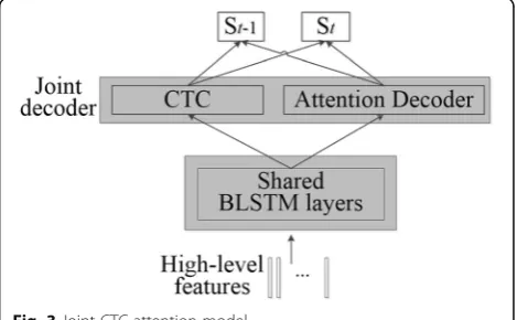
The network for feature extraction could also be consid-ered as intermediate supervision for our end-to-end models. Therefore, our features already contain high-level speech information; thus, it is not necessary to build a complex encoder that maps from raw inputs to phones. Following the setup in [17], we stack the joint CTC-attention model on top of our high-level features to build an end-to-end model, which is shown in Fig.3. This enables the utilization of the complementary ad-vantages of each model to improve the accuracy of the alignments.
We first define the symbol sets for the CTC model. Supposeπ is the sequence set decoded by CTC and de-note the tth symbol as πt whereπt∈{_,S1,…,ST}. T
de-notes the number of the character or phone symbol, and Stdenotes one of the characters or phone symbol in the original symbol set. The posteriors of a symbol πt at timetare computed over all inputsXwith bi-directional long short-term memory (BLSTM):
pðπtjXÞ ¼Softmax BLSTMð ð ÞX Þ ð5Þ
The distribution p(S|X) is modeled under conditional independent assumptions:
pCTCðSjXÞ ¼
X
π∈Φð ÞS0
pðπjXÞ≈ X
π∈Φð ÞS0
YT
t¼1
pðπtjXÞ;
ð6Þ
whereΦ(S') denotes all possible sequences.
For the attention-based model, the symbol set is γk∈ {<sos>,S1,…,ST, <eos>}. The posteriors p(S|X) of the
attention-based model are estimated directly with:
pattðSjXÞ≈
Y
k
p γkjγ1;…;γk−1;X
ð7Þ
Then, the loss functions of CTC and attention-based models to be optimized are defined as:
ℒCTC¼−lnpCTCðSjXÞ ℒatt¼−lnpattðSjXÞ
ð8Þ
The total loss function to be optimized is calculated as a combination of the logarithmic linear function of CTC and attention:
ℒ ¼λℒCTCþð1−λÞℒattention λ∈½0;1 ð9Þ
whereλis the linear weight of CTC loss.
It is known that the attention-based model decodes phone/character synchronously while CTC does it in a frame-wise way. Suppose that gl is a hypothesis with lengthl; this term could then be used to incorporate two scores. For the attention decoder, we compute the score of hypotheses in the beam search recursively:
αattð Þ ¼gl αattðgl−1Þ þ logp sðjgl−1;XÞ ð10Þ
wheresis the last character ofgl. Then, we use the CTC
prefix probability and obtain the CTC score as:
αCTCð Þ ¼gl logpðgl;…jXÞ ð11Þ
We combine the CTC score and attention score to-gether using one-pass decoding following the method in [13], and then αCTC(gl) can be combined with αatt(gl) using λ. The joint decoder gives the most likely phone sequenceSas follows:
S¼ arg max S λαCTC
gl
ð Þ þð1−λÞαattð Þgl
f g ð12Þ
3 Multi-head attention scored over multi-level outputs
Based on the model we have described in Section 2, we introduce our attention method utilizing multi-level in-formation. Previous studies on attentions have one thing in common: when calculating attention scores and the contexts, they only consider the outputs from the last layer. However, there is no clear evidence that the con-nections for alignments must be built between a certain layer of the encoder and a certain layer of the decoder. Moreover, we believe that the multi-head attentions are best suited to supplementary roles for our multi-level methods. The multi-head attentions play roles similar to those of kernels in the convolutional neural network (CNN). They are expected to extract multiple represen-tations in the encoder from different subspaces in paral-lel. This potentially allows attention-based models to capture embedded inner relations so that more accurate
attention scores can be provided. All of these facets indi-cate that the attention layer requires a better structure that can exploit as many inner relations as possible.
We will first introduce how the multi-level attention works; we propose making use of the last two consecu-tive layers of the encoder for the attention part. Our multi-level structure for the attention-based model is shown in Fig. 4. The inputs are DNN-based high-level features. The encoder is composed of a few layers of BLSTM cells and the decoder is composed of one layer of unidirectional LSTMs.
The attention mechanism is modified from the trad-itional structure of a location-based attention layer. The location-based attention includes three factors when cal-culating the score ek, t, i.e., the convolutional features fk
on previous weights, the hidden outputs for the decoder
s, and the last layer (nth) of outputs of the encoderhn. However, in Fig.4, the red dotted line starting from the second to the last layer of the encoder represents its extra contribution to the attention. Therefore, our calcu-lation of the attentions also depends on the extra out-puts of the encoder.
Let F and α denote a convolution filter and a T -di-mensional attention weight vector, respectively; then, the convolutional featuresfare calculated as follows:
f¼ Fα ð13Þ
Different from traditional attention scores, our design multiplies outputs from two consecutive layers of the encoder and inserts this term in the score. Let hn and hn−1denote the outputs from thenth layer and the (n‐
1)th layer, respectively; we usehn⊙hn−1to replacehn,
where the⊙operation is a Hadamard product. Here, we use a multiplicative operation instead of an addition or a concatenation operation because we intend to force a se-quential restriction to the attention. Because we use re-current layers as the encoder, a multiplication of consecutive layers could include long-term dependencies in the calculation of the attention score.
The multiplicative term hn⊙hn−1 enables the
atten-tion to be more sensible with regard to the multi-level outputs in case one layer of outputs is not enough and potentially embeds more long-term dependencies in the attention mechanism.
Then,ek,tis described as follows:
ek;t¼wT tanhVSsþVHðhn⊙hn−1Þ þVFfk;tþb
ð14Þ
where w, VS, VH, andVFare trainable weight matrices. Letαk,tdenote the attention weights connectingkth
en-coder outputs andtth decoder inputs. It is scaled with a
αk;t¼ exp γek;t
PT
t¼1 exp γek;t
ð15Þ
Additionally, let rk denote the context term used to decode the kth symbol. It integrates encoder outputs from two layers using attention weights:
rk¼
XT
t¼1αk;t hn;tþhn−1;t
ð16Þ
wherehn, tand hn‐1, tare the tth output vectors in the nth layer and (n‐1)th layer, respectively. We add the additionalhn‐1,tterm in Eq. (16) to form residual
con-nections and tied weights for the attention layer. This could alleviate the degradation of weights potentially brought about by our complex attention structure.
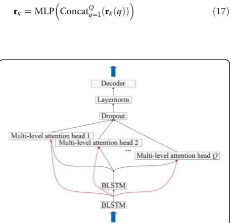
After the introduction of our multi-level method, we will incorporate multi-level outputs into multi-head at-tentions and show the schematic structure of the atten-tion layer in Fig.5.
As shown, our multi-head attention is a modified com-bination of location-based attentions. The attention score of each head relies on double outputs. Let Q de-note the total number of heads, and let rk(q) replace rk as the context of the qth attention head, the total
context is output from an MLP with a sum of contexts of each head as input:
rk¼MLP ConcatQq¼1ðrkð Þq Þ
ð17Þ Fig. 4Multi-level attention-based model
To alleviate the overfitting problem caused by increas-ing parameters, dropout is applied to connections be-tween context and the decoder. In addition, layer normalization [20] is added to normalize the distribution of the sum of all contexts. In addition, the original multi-head attentions in [18] use an additional convolu-tional operation over the encoder outputs.
Then, posteriors for the attention-based model are output from the decoder vias,rk,hn, andhn−1:
p sðkjs1;…;sk−1;XÞ ¼Decoderðs;rk;hn;hn−1Þ ð18Þ
What should be noticed in our method is that some configurations of the model may vary from the original joint CTC-attention model. The multi-task learning weight λ in the multi-head multi-level attention model should be lower because this attention type is expected to impose more restrictions on alignment; therefore, there would be less need for CTC. Additionally, we choose to use a deeper encoder and decoder for this at-tention type referring to the configurations in [18].
4 Experiments and analysis
4.1 Dataset and evaluation measurement
We test our methods on TIMIT, WSJ, and LibriSpeech in our experiments. For TIMIT, we followed the com-mon setup. All SA sentences were removed. We select 46,250 speakers, as well as 24 speakers each for the training set, dev set, and core test set. On the WSJ data-set, we used the standard setup: “si284” for the training set, “dev93” for validation, and“eval92” for the test set. No extra dataset is used. The language model is trained with all transcriptions from the training set. For LibriS-peech, we train with 960 h of data and evaluate on the “test clean”set.
Phone error rate (PER) is adopted to measure per-formance in TIMIT, and word error rate (WER) is adopted to measure performances in WSJ and LibriS-peech. Both scores are calculated with the following equation:
PER=WER¼nInsþnDelþnSub
N 100% ð19Þ
where nIns, nDel, andnSub are the numbers of insert
er-rors, delete erer-rors, and substitute erer-rors, respectively. N is the total number of words/phones in the ground truth labels.
4.2 Experimental tools
The extraction of low-level acoustic features and the training of GMMs are implemented with Kaldi [21]. We use Theano [22] and the PyMF toolkit [23] to train the DNN and apply CNMF. Our end-to-end speech recogni-tion systems are built with the Chainer [24] backend on
ESPnet [25]. Additionally, we use a single NVIDIA GeForce GTX 1080Ti to accelerate training for networks.
4.3 Experiments on TIMIT
In this part, we test our methods on the TIMIT dataset. Experiments in this part are extensions of our previous work in [17]. In short, all models are trained over high-level features with transfer learning. Except for attention layers, we copy all the configurations of the feature ex-traction and the end-to-end models from [17]. There-fore, we do not introduce many experimental details in this part.
The only difference lies in the attention layer. Instead of using a normal location-based attention, we test on location-based attention over multi-level outputs and multi-head location-based attention and their combination.
System P0 is our best system in [17]. System P1 is based on P0, with multi-level location-based attention instead of a normal location-based attention, and its out-puts from the last two consecutive layers of the encoder are included in calculations. System P2 is based on P0, with four-head location-based attention. System P3 com-bines the multi-level outputs with multi-head attention. All heads include double outputs from the encoder. We list some of the important configurations for TIMIT ex-periments in Table1.
As mentioned in Section 2.2, two important settings should be highlighted, which are the depth of the net-work and the MTL λ. We also notice a fact from [18] that as many as six layers were needed for multi-head at-tentions. Therefore, we use deeper networks for our sys-tems containing multi-head attentions. We should emphasize that adding more encoder and decoder layers does not improve the performance of the baseline, and the deeper encoder and decoder only work well with multi-head attentions (we do not discuss in detail but we conducted experiments to confirm). Therefore, the factor of a deeper structure should be excluded from the improvement contribution. Moreover, lower λ is better for our proposed attentions. The multi-head attention scored over multi-level outputs brings more restrictions, which could compensate for the need for CTC.
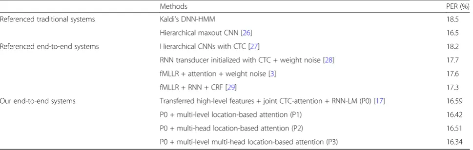
The results on TIMIT are shown in Table2.
4.4 Experiments on WSJ
smoothing method is applied with a weight of 0.05. Moreover, the MTLλ is set to 0.2, the decoding weight for CTC is 0.3, and the scaling factor for the recurrent neural network language model (RNN-LM) is 1.0 for all joint models. For the location-based attentions, the number of filters for convolutional features is 100, and the number of channels is 10.
We train a word-level RNN-LM [31] to help decode all end-to-end systems. The RNN is a 1-layer LSTM with 1000 units. The RNN-LM is trained using stochas-tic gradient descent (SGD) for 20 epochs with a batch size of 100. The softmax layer predicts 65,000-dimen-sional output values, which means that the vocabulary size is 65,000.
4.4.1 Baseline setup
The configuration for the baseline system is that which performs best in the ESPnet WSJ example, which is a joint CTC-attention-based system. However, we rerun this example with a Chainer version (the original is a PyTorch version) to make it consistent with other exper-iments in this paper. The input features are 40 Mel filter banks with delta and delta-delta components. The en-coder is a combination of a VGG net and a BLSTM. The VGG net has two components, and each component has two 2D convolutional layers with a 2D max pooling layer. The stride for max pooling is (2, 2) which means two steps of stride in each axis. A rectified linear unit (ReLU) is used as the activation function on top of each convolutional layer. The convolutional parameters are described in Table3.
The RNN of the shared encoder is composed of 4 layers of BLSTM with 320 units in each direction and layer. Add attention is used, and the attention layer has 320 units. The decoder is a 1-layer LSTM with 300 units in each layer. The batch size during training was set to 30.
Table 4 lists the performance of the baseline system K0.
4.4.2 Experiments on high-level features
We then experiment on our high-level feature-based ap-proach. The network for feature extraction is a 5-hidden layer DNN. Each layer has 1026 input units and 342 out-put units with a max pooling size of 3. Dropout is ap-plied to each hidden layer with a rate of 0.2. To obtain labels for DNN, we first build a GMM. The GMM is trained using linear discriminative analysis (LDA), max-imum linear logistic transformation (MLLT), and speaker adaptive training (SAT) with 13 MFCC features. Then, DNN is supervised by alignments of senones gen-erated by each GMM. The initial learning rate was kept at 0.2 for the first 8 epochs, and after that, it was decayed by half when the validation error did not de-cline. The training stops when the validation error finally increases.
We build a narrow layer for the DNN with CNMF. We follow the exact same setting in [16, 17] for factorization, which is applying CNMF on the weight matrix from the second to the last hidden layer. The weight matrix is factorized into 40 dimensions after 5000 iterations of training.
Table 1Important configurations for TIMIT experiments
System CTC encoder layers Attention encoder layers Decoder layers MTLλ
P1 2 3 1 0.3
P2 2 3 1 0.2
P3 3 4 2 0.2
Table 2Comparisons on the TIMIT core test set
Methods PER (%)
Referenced traditional systems Kaldi’s DNN-HMM 18.5
Hierarchical maxout CNN [26] 16.5
Referenced end-to-end systems Hierarchical CNNs with CTC [27] 18.2
RNN transducer initialized with CTC + weight noise [28] 17.7
fMLLR + attention + weight noise [3] 17.6
fMLLR + RNN + CRF [29] 17.3
Our end-to-end systems Transferred high-level features + joint CTC-attention + RNN-LM (P0) [17] 16.59
P0 + multi-level location-based attention (P1) 16.42
P0 + multi-head location-based attention (P2) 16.51
After the previous steps, these high-level features are sent to joint CTC-attention models for end-to-end train-ing. We only build shallow RNN networks on top of our high-level features. According to our experience in [17], we set a 3-layer BLSTM for the CTC encoder and a 2-layer BLSTM for the attention-based encoder. The joint decoder is a 1-layer LSTM. BLSTM and LSTM both have 320 cells in each layer and direction. We use location-based attention, and the attention layer has 160 cells. The BLSTM of the encoder and attention layer are both regularized with a dropout rate of 0.2 during train-ing. We name this system K1, and its result is shown in the second line of the third block in Table4.
4.4.3 Further experiments on multi-level multi-head attentions
We further experiment on our proposed attention methods. All attention layers have 160 units with a drop-out rate of 0.2 and a layer normalization on top of the context rk. The model is still a joint CTC-attention model upon high-level features. Except for attentions, the rest of the configuration of end-to-end models re-mains the same as the previous settings.
First, we test the multi-level location-based attention and the multi-head attention separately. System K2 is based on K1 with multi-level location-based attention, and its outputs from the last two consecutive layers of the encoder are included in the calculations. System K3
is based on K1 with four-head location-based attention. System K4 combines the level outputs with multi-head attention. All multi-heads include double outputs from the encoder. We list the best configurations for these variables in Table5.
As analyzed in TIMIT experiments, we choose various empirical settings for the number of layers and MTL λ in the WSJ experiments. We list the results of the WSJ systems in Table4.
4.5 Experiments on LibriSpeech
Finally, we experiment on larger-scale data, which is 960 h of training data in LibriSpeech, to further demon-strate the effectiveness of our methods. Models in LibriSpeech were also trained with characters. The beam size for decoding is 20. We use Adadelta for the optimizer with no label smoothing method. The MTLλ and the decoding weight are both set to 0.5, and the scaling factor for the RNN-LM is 0.7 for all joint models.
We use byte pair encoding (BPE) [39] to create 5000 subword units as the output targets of the decoder. The model is a 1-layer LSTM with 1024 units and is trained using SGD for 20 epochs with a batch size of 1024.
For the baseline, we set 1024 units for BLSTM in each layer and direction with 5 layers and 1024 units for the attention layer. The rest of the configuration of the base-line system follows the basebase-line settings in WSJ.
Table 3Parameters of convolutional layers in WSJ experiments
Layer Input channels Output channels Kernel size Stride
Convolutional layer 1 1 64 (3, 3) (1, 1)
Convolutional layer 2 64 64 (3, 3) (1, 1)
Convolutional layer 3 64 128 (3, 3) (1, 1)
Convolutional layer 4 128 128 (3, 3) (1, 1)
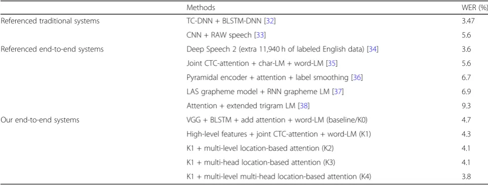
Table 4Comparisons on WSJ“eval92”
Methods WER (%)
Referenced traditional systems TC-DNN + BLSTM-DNN [32] 3.47
CNN + RAW speech [33] 5.6
Referenced end-to-end systems Deep Speech 2 (extra 11,940 h of labeled English data) [34] 3.6
Joint CTC-attention + char-LM + word-LM [35] 5.6
Pyramidal encoder + attention + label smoothing [36] 6.7
LAS grapheme model + RNN grapheme LM [37] 6.9
Attention + extended trigram LM [38] 9.3
Our end-to-end systems VGG + BLSTM + add attention + word-LM (baseline/K0) 4.7
High-level features + joint CTC-attention + word-LM (K1) 4.3
K1 + multi-level location-based attention (K2) 4.1
K1 + multi-head location-based attention (K3) 4.1
For our high-level feature-based system, we also set a 3-layer BLSTM for the CTC encoder and a 2-layer BLSTM for the attention-based encoder. The joint de-coder is a 1-layer LSTM. They have 1024 cells in each layer and direction. We use location-based attention, and the attention layer has 512 cells. A dropout rate of 0.2 is applied to both BLSTM layers and attention layers. Like the settings in WSJ, we reduce the training and de-coding weight for CTC, with both weights set to 0.4, for multi-head and multi-level attentions. For our proposed attention methods, the rest of the configuration of the end-to-end models remains the same as in WSJ.
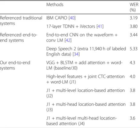
We name our baseline and our basic high-level feature-based systems as J0 and J1. For the rest of the systems, J2, J3, and J4 represent our multi-head attention system, multi-level attention system, and their combin-ation, respectively. The results on LibriSpeech are listed in Table6.
4.6 Results and discussions
Table 2shows the results of all referenced methods and our methods on TIMIT. The baseline system “P0 + RNN-LM”has the best performance in [17]. It is a joint CTC-attention model with a normal location-based at-tention. Its inputs are high-level features extracted using
transfer learning. We can see that the performance is slightly worse than that of the state-of-the-art system.
When using the attentions proposed in this paper to replace the original attention, the PERs were further re-duced. We notice that the multi-level location-based at-tention performs better than the multi-head location-based attention. This is probably because the parameters in the multi-head attention model are too much for a small corpus such as TIMIT. Finally, the system with a multi-level multi-head location-based attention achieved the best performance compared with all listed methods. This is an interesting fact because the multi-level con-nections bring even more parameters for training which is supposed to degrade the performance in TIMIT. We further implement three significance tests, including the matched pair sentence segment test, the signed pair comparison test, and the Wilcoxon signed-rank test using the SCTK toolkit.1Both P1 and P2 fail to reach a 5% level of significance of difference compared with P0. For our best system, P3 reaches a 5% level of significance in both MP and SI tests, while no significant difference is found in the WI test.
However, the improvement brought by this combin-ation demonstrates that, although our attention mechan-ism is complicated in connections, it could bring more benefit than harm even in limited resource cases.
Table 4 shows the results of all referenced methods and our methods on WSJ. We can see that the perform-ance of the baseline system K0 is already at a good level. When high-level features are introduced, our system K1 outperforms the baseline system as well as many present end-to-end models. This further demonstrates that high-level knowledge could be transferred into end-to-end models, which was also proved in our previous work [17]. Both systems K2 and K3 perform equally better than our previous systems. However, two methods help in different ways. The multi-level location-based atten-tion could strengthen long-term restricatten-tions due to the multiplicative term. The multi-head attention extracts inner relations embedded in the encoder and therefore includes a self-restriction.
When we use a combination of level and multi-head methods in the attention layer in system K4, the WER is further reduced and is only 0.2% worse than the
Table 5Important configurations for WSJ experiments
System CTC encoder layers Attention encoder layers Decoder layers MTLλ
K1 2 3 1 0.2
K2 2 3 1 0.1
K3 3 4 2 0.1
K4 3 4 2 0.1
Table 6Comparisons on LibriSpeech“test clean”
Methods WER
(%)
Referenced traditional systems
IBM CAPIO [40] 3.19
17-layer TDNN + iVectors [41] 3.80
Referenced end-to-end systems
End-to-end CNN on the waveform + conv LM [42]
3.44
Deep Speech 2 (extra 11,940 h of labeled English data) [34]
5.33
Our end-to-end systems
VGG + BLSTM + add attention + word-LM (baseline/J0)
4.3
High-level features + joint CTC-attention + word-LM (J1)
4.0
J1 + multi-level location-based attention (J2)
3.8
J1 + multi-head location-based attention (J3)
3.8
J1 + multi-level multi-head location-based attention (J4)
3.6
WER of the “Deep Speech 2” model in [34]. However, it should be noted that the “Deep Speech 2” model is trained on a much larger scale of dataset and apparently has a much deeper network with more computational components, while our method is more simplified with only a few layers in the RNN, and the model is trained only on 81 h of the WSJ dataset. Considering the gap be-tween the training data, we believe that our results are totally acceptable. We also apply three significance tests to our results. The differences among the five systems in Table 4 are all statistically significant at a 5% level in three tests.
Table 6 shows comparisons of the LibriSpeech “test clean”set. Our high-level feature-based system still beats the baseline system. The results of J2 and J3 show a similar conclusion to that which we get in WSJ, indicat-ing that multi-level attention and multi-head attention could play similar roles in improving the attention-based model. When they are combined as a more complex attention layer, the performance also further improves, just like the case in WSJ. Although our method cannot compare with the state-of-the-art system that combines multiple systems, it performs closely to the best refer-enced end-to-end approach, with only a gap of 0.16% in WER. Again, we find that the differences between the five systems in Table6are all statistically significant at a 5% level in three significance tests. The improvement brought by the combination of head and multi-level attention demonstrates that two different attention types solve different problems in attention-based models and are complementary to each other. This greatly broadens the research of attention structures.
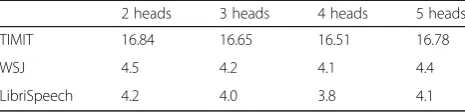
Beyond all experiments above, we further experiment on different numbers of heads ranged from two to five heads. We do not use more than five heads due to mem-ory limits. The results on single attention are summed in Table 7. The results of multi-level attention are listed in Table8.
We can see that the four-head attention performs the best among all settings in all three corpora. Lesser heads may not provide enough information, and more heads probably brings intermediate redundancy. This further demonstrates why we choose an empirical setting of four heads in multi-head attentions.
5 Conclusion
In this paper, we mainly propose the advancement of the attention mechanism in joint CTC-attention-based speech recognition. In the first phase, we adopt a high-level feature-based joint model from our previous work [17]. The only difference is that we do not use multi-lingual pre-training for DNN.
In the second phase, we introduce a new attention type for our end-to-end models. We add extra connections for the second to the last layer of the encoder and then apply multi-head attentions. Unlike other normal attention types, this attention is scored over multi-level outputs of the RNN and therefore brings extra long-term dependen-cies on the attention. Experiments on TIMIT show that all of our models perform better than all referenced methods and prove the robustness of our method. Further experiments on WSJ and LibriSpeech show that our atten-tion mechanism could achieve the best performance among all end-to-end methods without data augmenta-tion, and it is only slightly worse than the state-of-the-art performance. In the future, we would study other ways of utilizing multi-level information [43].
Abbreviations
BLSTM:Bi-directional long short-term memory; BPE: Byte pair encoding; CNMF: Convex nonnegative matrix factorization; CNN: Convolutional neural network; CTC: Connectionist temporal classification; DNN: Deep neural network; GMMs: Gaussian mixture models; HMMs: Hidden Markov models; LDA: Linear discriminative analysis; MLLT: Maximum linear logistic transformation; MLP: Multi-layer perceptron; NMF: Nonnegative matrix factorization; NTM: Neural Turing machines; PER: Phone error rate; ReLU: Rectified linear unit; RNN-LM: Recurrent neural network language model; SAT: Speaker adaptive training; SGD: Stochastic gradient descent; WER: Word error rate
Acknowledgements
We also would like to express our thanks to the professional writing services provided by Springer Nature Author Services, which improves the writing quality of our manuscript.
Authors’contributions
CXQ and DQ conceived and designed the study. CXQ performed the experiments. CXQ and DQ wrote the paper. CXQ, DQ, and WLZ reviewed and edited the manuscript. All authors read and approved the manuscript.
Authors’information
Chu-Xiong Qin was born in Shijiazhuang, China, in 1991. He received his BS and MS degrees in Information and Communication from the National Digital Switching System Engineering and Technological R&D Center, Zhengzhou, China, in 2013 and 2016, respectively. He is currently working towards his PhD degree in Speech Recognition at the National Digital Switching System Engineering and Technological R&D Center. His research interests are speech signal processing, continuous speech recognition, and machine learning.
Table 7Comparisons on different heads for single attention
2 heads 3 heads 4 heads 5 heads
TIMIT 16.84 16.65 16.51 16.78
WSJ 4.5 4.2 4.1 4.4
LibriSpeech 4.2 4.0 3.8 4.1
Table 8Comparisons on different heads for multi-level attention
2 heads 3 heads 4 heads 5 heads
TIMIT 16.73 16.52 16.34 16.60
WSJ 4.2 4.0 3.8 4.0
Wen-Lin Zhang received his PhD degree in Information and Communication Engineering from the National Digital Switching System Engineering and Technological R&D Center, Zhengzhou, China, in 2014. He is a lecturer at the National Digital Switching System Engineering and Technological R&D Center. His research interest is speech signal processing.
Dan Qu received her MS degree in Communication and Information System from Xi’an Information Science and Technology Institute, Xi’an, China, in 2000 and her PhD degree in Information and Communication Engineering from the National Digital Switching System Engineering and Technological R&D Center, Zhengzhou, China, in 2005. She is an associate professor at the National Digital Switching System Engineering and Technological R&D Center. Her research interests are speech signal processing and pattern recognition.
Funding
This work was supported in part by the National Natural Science Foundation of China (No. 61673395 and No. 61403415), Natural Science Foundation of Henan Province (No. 162300410331), and the China Postdoctoral Science Foundation (No. 2016 M602975).
Availability of data and materials
All data used in our experiments are all available. The TIMIT is available as LDC corpus LDC93S1, which is one of the original clean speech databases. The WSJ corpus is available from the LDC as either [catalog numbers LDC93S6A (WSJ0) and LDC94S13A (WSJ1)] or [catalog numbers LDC93S6B (WSJ0) and LDC94S13B (WSJ1)]. The LibriSpeech is available for download for free athttp://www.openslr.org/12/. It was prepared as a speech recognition corpus by Vassil Panayotov.
Competing interests
The authors declare that they have no competing interests.
Received: 2 April 2019 Accepted: 25 September 2019
References
1. L.R. Rabiner, A tutorial on hidden Markov models and selected applications in speech recognition. Proc. IEEE77(2), 257–286 (1989)
2. L.R. Rabiner, B.H. Juang,Fundamentals of speech recognition, vol 14 (PTR Prentice Hall, Englewood Cliffs, 1993)
3. J.K. Chorowski, D. Bahdanau, D. Serdyuk, K. Cho, and Y. Bengio, Attention-based models for speech recognition n Advances in Neural Information Processing Systems (NIPS), 2015, pp. 577–585
4. Y. Miao, M. Gowayyed, and F. Metze, EESEN: end-to-end speech recognition using deep RNN models and WFST-based decoding, Automatic Speech Recognition and Understanding (ASRU), 2015 IEEE Workshop on. IEEE, 2015 5. C. C. Chiu, T. N. Sainath, Y. Wu, R. Prabhavalkar, P. Nguyen, Z. Chen, A.
Kannan, R. J. Weiss, K. Rao, K. Gonina, et al., State-of-the-art speech recognition with sequence-to-sequence models, 2018 IEEE International Conference on Acoustics, Speech and Signal Processing (ICASSP), 2018 6. D. Bahdanau, K. Cho, and Y. Bengio, Neural machine translation by jointly
learning to align and translate, arXiv preprint arXiv:1409.0473 (2014) 7. Luong, Minh-Thang, Hieu Pham, and Christopher D. Manning, Effective
approaches to attention-based neural machine translation, arXiv preprint arXiv:1508.04025 (2015)
8. W. Chan, N. Jaitly, Q. Le, and O. Vinyals, Listen, attend and spell: a neural network for large vocabulary conversational speech recognitione, in IEEE International Conference on Acoustics, Speech and Signal Processing (ICASSP), 2016, pp. 4960–4964
9. P. Ren, Z. Chen, Z. Ren, et al., (2017), Leveraging contextual sentence relations for extractive summarization using a neural attention model, in Proceedings of the 40th International ACM SIGIR Conference on Research and Development in Information Retrieval, pp. 95–104
10. Y. Cui, Z. Chen, S. Wei, et al., Attention-over-attention neural networks for reading comprehension arXiv preprint arXiv:1607.04423(2016)
11. J. Gehring, M. Auli, D. Grangier, et al., Convolutional sequence to sequence learning, arXiv preprint arXiv:1705.03122, 2017
12. S. Watanabe, T. Hori, S. Kim, et al., Hybrid CTC/attention architecture for end-to-end speech recognition. IEEE. J. Select. Topics. Signal. Process.11(8), 1240–1253 (2017)
13. T. Hori, S. Watanabe, and J. Hershey, Joint CTC/attention decoding for end-to-end speech recognition, Proceedings of the 55th Annual Meeting of the Association for Computational Linguistics (Volume 1: Long Papers). 1. 2017 14. S. Kim, T. Hori, S. Watanabe, Joint CTC-attention based end-to-end speech
recognition using multi-task learning, Acoustics, Speech and Signal Processing (ICASSP), 2017 IEEE International Conference on. IEEE, 2017: 4835–4839
15. T. Hori, S. Watanabe, Y. Zhang, et al., Advances in joint CTC-attention based end-to-end speech recognition with a deep CNN encoder and RNN-LM, arXiv preprint arXiv:1706.02737 (2017)
16. C. Qin, and L. Zhang, Deep neural network based feature extraction using convex-nonnegative matrix factorization for low-resource speech recognition, in Information Technology, Networking, Electronic and Automation Control Conference (ITNEC), 2016
17. C.-X. Qin, Q. Dan, L.-H. Zhang, Towards end-to-end speech recognition with transfer learning. EURASIP J Audio. Speech. Music. Process18, 1–9 (2018) 18. A. Vaswani, N. Shazeer, N. Parmar, J. Uszkoreit, L. Jones, A.N. Gomez, et al.,
Attention is all you need. Adv. Neural. Inf. Process. Syst.(NIPS)2017, 5998– 6008 (2017)
19. C.H. Ding, T. Li, M.I. Jordan, Convex and semi-nonnegative matrix factorizations. IEEE Trans. Pattern Anal. Mach. Intell.32(1), 45–55 (2010) 20. J. L. Ba, J. R. Kiros, and G. E. Hinton, Layer normalization, arXiv preprint arXiv:
1607.06450 (2016)
21. D. Povey, A. Ghoshal, G. Boulianne, et al., The Kaldi speech recognition toolkit, IEEE 2011 workshop on automatic speech recognition and understanding. No. EPFL-CONF-192584. IEEE Signal Processing Society, 2011 22. the Montreal Institute for Leaning Algorithms (MILA), Theano,http://www.
deeplearning.net/software/theano/, 2017
23. Christian Thurau, PyMF - Python Matrix Factorization Module,https://github. com/cthurau/pymf, 2013
24. S. Tokui, K. Oono, S. Hido, J. Clayton,Chainer: a next-generation open source framework for deep learning, Proceedings of Workshop on Machine Learning Systems (LearningSys) in The Twenty-ninth Annual Conference on Neural Information Processing Systems (NIPS)(2015)
25. S. Watanabe, T. Hori, S. Karita, et al., ESPnet: end-to-end speech processing toolkit, arXiv preprint arXiv:1804.00015, 2018
26. L. Tóth, Phone recognition with hierarchical convolutional deep maxout networks. EURASIP J Audio. Speech. Music. Process. (1), 25 (2015) 27. Y. Zhang, M. Pezeshki, P. Brakel, S. Zhang, C. L. Y. Bengio, and A. Courville,
Towards end-to-end speech recognition with deep convolutional neural networks, arXiv preprint arXiv: 1701.02720, 2017
28. A. Graves, A. R. Mohamed, and G. Hinton, Speech recognition with deep recurrent neural networks, in IEEE International Conference on Acoustics, Speech and Signal Processing (ICASSP), pp. 6645–6649, 2013
29. L. Lu, L. Kong, C. Dyer, N. A. Smith, Multi-task learning with CTC and segmental CRF for speech recognition, arXiv preprint arXiv: 1702.06378, 2017
30. R. Pascanu, T. Mikolov, and Y. Bengio, On the difficulty of training recurrent neural networks, arXiv preprint arXiv: 1211.5063, 2012
31. T. Hori, J. Cho, and S. Watanabe, End-to-end speech recognition with word-based RNN language models, arXiv preprint arXiv:1808.02608, 2018 32. W. Chan, and I. Lane, Deep recurrent neural networks for acoustic
modelling, arXiv preprint arXiv:1504.01482(2015)
33. D. Palaz, M. M. Doss, and R. Collobert, Convolutional neural networks-based continuous speech recognition using raw speech signal, Acoustics, Speech and Signal Processing (ICASSP), 2015 IEEE International Conference on. IEEE, 2015 34. D. Amodei, R. Anubhai, E. Battenberg, et al, Deep Speech 2: end-to-end speech recognition in English and Mandarin, Computer Science, 2015 35. T. Hori, S. Watanabe, and J. R. Hershey, Multi-level language modeling and decoding for open vocabulary end-to-end speech recognition, Automatic Speech Recognition and Understanding Workshop (ASRU), 2017 IEEE. IEEE, 2017 36. J. Chorowski, and N. Jaitly, Towards better decoding and language model
integration in sequence to sequence models, arXiv preprint arXiv:1612. 02695, 2016
37. A. Kannan, Y. Wu, P. Nguyen, T. N. Sainath, Z. Chen, and R. Prabhavalkar, An analysis of incorporating an external language model into a sequence-to-sequence model, In 2018 IEEE International Conference on Acoustics, Speech and Signal Processing (ICASSP), 2018
39. R. Sennrich, B. Haddow, and A. Birch, Neural machine translation of rare words with subword units, in ACL, Berlin, 2016, pp. 1715–1725
40. K. J. Han, A. Chandrashekaran, J. Kim, & I. Lane, The CAPIO 2017 conversational speech recognition system. arXiv preprint arXiv:1801.00059, 2017
41. D. Povey, G. Cheng, Y. Wang, K. Li, H. Xu, M. Yarmohamadi, and S. Khudanpur, Semi-orthogonal low-rank matrix factorization for deep neural networks. In Proceedings of the 19th Annual Conference of the International Speech Communication Association (INTERSPEECH 2018), Hyderabad, India
42. N. Zeghidour, Q. Xu, V. Liptchinsky, N. Usunier, G. Synnaeve, and R. Collobert. Fully convolutional speech recognition. arXiv preprint arXiv:1812. 06864, 2018
43. Y. Tang, G. Ding, J. Huang, X. He, & B. Zhou, Deep speaker embedding learning with multi-level pooling for text-independent speaker verification, arXiv preprint arXiv:1902.07821, 2019
Publisher’s Note