R E S E A R C H
Open Access
Iterative approximation of solutions for
proximal split feasibility problems
Yekini Shehu
1, Gang Cai
2*and Olaniyi S Iyiola
3*Correspondence: [email protected] 2School of Mathematics Science, Chongqing Normal University, Chongqing, 400047, China Full list of author information is available at the end of the article
Abstract
In this paper, our aim is to introduce a viscosity type algorithm for solving proximal split feasibility problems and prove the strong convergence of the sequences generated by our iterative schemes in Hilbert spaces. First, we prove strong convergence result for a problem of finding a point which minimizes a convex functionfsuch that its image under a bounded linear operatorAminimizes another convex functiong. Secondly, we prove another strong convergence result for the case where one of the two involved functions is prox-regular. In all our results in this work, our iterative schemes are proposed by way of selecting the step sizes such that their implementation does not need any prior information about the operator norm because the calculation or at least an estimate of the operator normAis not an easy task. Finally, we give a numerical example to study the efficiency and
implementation of our iterative schemes. Our results complement the recent results of Moudafi and Thakur (Optim. Lett. 8:2099-2110, 2014, doi:10.1007/s11590-013-0708-4) and other recent important results in this direction.
MSC: 49J53; 65K10; 49M37; 90C25
Keywords: proximal split feasibility problems; Moreau-Yosida approximate; prox-regularity; strong convergence; Hilbert spaces
1 Introduction
In this paper, we shall assume thatHis a real Hilbert space with inner product·,·and norm · . LetIdenote the identity operator onH. LetCandQbe nonempty, closed, and convex subsets of real Hilbert spacesHandH, respectively. Thesplit feasibility problem
(SFP) is to find a point
x∈Csuch thatAx∈Q, (.)
whereA:H→H is a bounded linear operator. The SFP in finite-dimensional Hilbert
spaces was first introduced by Censor and Elfving [] for modeling inverse problems which arise from phase retrievals and in medical image reconstruction []. The SFP attracts the attention of many authors due to its application in signal processing. Various algorithms have been invented to solve it (see, for example, [–] and references therein). For a more current and up-to-date survey on split feasibility problems, please see [].
Note that the split feasibility problem (.) can be formulated as a fixed point equation by using the fact
PC
I–γA∗(I–PQ)Ax∗=x∗; (.)
that is,x∗ solves the SFP (.) if and only ifx∗ solves the fixed point equation (.) (see [] for the details). This implies that we can use fixed point algorithms (see [–]) to solve SFP. A popular algorithm that solves the SFP (.) is due to Byrne’s CQ algorithm [] which is found to be a gradient-projection method (GPM) in convex minimization. Subsequently, Byrne [] applied Krasnoselskii-Mann iteration to the CQ algorithm, and Zhao and Yang [] applied Krasnoselskii-Mann iteration to the perturbed CQ algorithm to solve the SFP. It is well known that the CQ algorithm and the Krasnoselskii-Mann al-gorithm for a split feasibility problem do not necessarily converge strongly in the infinite-dimensional Hilbert spaces.
Our goal in this paper is to study the more general case of proximal split minimization problems and to investigate the strong convergence properties of the associated numerical solutions. To begin with, let us consider the following problem: Find a solutionx∗∈H
such that
min x∈H
f(x) +gλ(Ax)
, (.)
whereH,Hare two real Hilbert spaces,f :H→R∪ {+∞},g:H→R∪ {+∞}two
proper, convex, lower-semicontinuous functions andA:H→Ha bounded linear
oper-ator,gλ(y) =minu∈H{g(u) +
λu–y}stands for the Moreau-Yosida approximate of the
functiongof parameterλ.
Observe that by takingf =δC (defined as δC(x) = ifx∈Cand +∞otherwise),g= δQthe indicator functions of two nonempty, closed, and convex setsC,QofH andH,
respectively, problem (.) reduces to
min x∈H
δC(x) + (δQ)λ(Ax)
⇔ min x∈C
λ(I–PQ)(Ax)
(.)
which, whenC∩A–(Q)=∅, is equivalent to (.).
By the differentiability of the Yosida approximategλ, see for instance [], we have the
additivity of the subdifferentials and thus we can write
∂f(x) +gλ(Ax)
=∂f(x) +A∗∇gλ(Ax) =∂f(x) +A∗
I–proxλg
λ
(Ax).
This implies that the optimality condition of (.) can then be written as
∈λ∂f(x) +A∗(I–proxλg)(Ax), (.) whereproxλg =argminu∈H
{g(u) +
λu–y
}stands for the proximal mapping ofgand
the subdifferential off atxis the set
∂f(x) :=u∈H:f(y)≥f(x) +u,y–x,∀y∈H
The inclusion (.) in turn yields the following equivalent fixed point formulation:
proxμλfx∗–μA∗(I–proxλg)Ax∗=x∗. (.) To solve (.), (.) suggests us to consider the following split proximal algorithm:
xn+=proxμnλf
xn–μnA∗(I–proxλg)
Axn. (.)
Based on an idea introduced in work of Lopez et al. [], Moudafi and Thakur [] recently proved weak convergence results for solving (.) in the case argminf ∩ A–(argming)=∅, or in other words: in finding a minimizerx∗off such thatAx∗ min-imizesg, namely
x∗∈argminf such thatAx∗∈argming, (.)
f,gbeing two proper, lower-semicontinuous convex functions,argminf :={¯x∈H:f(x¯)≤ f(x),∀x∈H} and argming:={¯y∈H:g(¯y)≤g(y),∀y∈H}. We will denote the
solu-tion set of (.) by . Concerning problem (.), Moudafi and Thakur [] introduced a new way of selecting the step sizes: Set θ(xn) :=∇h(x)+∇l(x) with h(x) =
(I–proxλg)Ax,l(x) = (I–proxλμnf)xand introduced the following split proximal algorithm.
Split proximal algorithm Given an initial pointx∈H. Assume thatxnhas been con-structed andθ(xn)= , then computexn+via the rule
xn+=proxλμnf
xn–μnA∗(I–proxλg)Axn
, n≥, (.)
where the step sizeμn:=ρnh(xnθ)+(xnl(xn) )with <ρn< . Ifθ(xn) = , thenxn+=xnis a solution of (.) and the iterative process stops, otherwise, we setn:=n+ and go to (.).
Using the split proximal algorithm (.), Moudafi and Thakur [] proved the following
weak convergencetheorem for approximating a solution of (.).
Theorem . Assume that f and g are two proper convex lower-semicontinuous functions and that(.)is consistent(i.e.,=∅).If the parameters satisfy the conditions ≤ρn≤
h(xn)
h(xn)+l(xn)– (for some > small enough),then the sequence{xn}generated by(.)weakly converges to a solution of (.).
Furthermore, Moudafi and Thakur [] assumedfto be convex and allowed the function
gto be nonconvex. In the case of indicator functions of subsets withA=I, such a situation is encountered in a numerical solution to phase retrieval problem in inverse scattering [] and is therefore of great practical interest. They considered the more general problem of finding a minimizerx¯off such thatAx¯is a critical point ofg, namely
∈∂f(¯x) such that ∈∂pg(Ax¯), (.)
Split proximal algorithm Given an initial pointx∈H. Assume thatxnhas been con-structed andθ(xn)= , then computexn+via the rule
xn+=proxλnμnf
xn–μnA∗(I–proxλng)Axn
, n≥, (.)
where the step sizeμn:=ρnh(xnθ)+(xnl(xn) )with <ρn< . Ifθ(xn) = , thenxn+=xnis a solution of (.) and the iterative process stops, otherwise, we setn:=n+ and go to (.).
Using (.), Moudafi and Thakur [] proved the followingweak convergencetheorem for the approximation of the solution of (.).
Theorem . Assume that f is a proper convex lower-semicontinuous function,g is
lo-cally lower-semicontinuous at Ax¯,prox-bounded,and prox-regular at Ax for¯ v¯= with
¯
x a point which solves (.)and A a bounded linear operator which is surjective with a dense domain. If the parameters satisfy the following conditions: ∞n=λn <∞ and infnρn(h(xnh)+(xnl()xn)–ρn) > and ifx–x¯is small enough,then the sequence{xn} gener-ated by(.)weakly converges to a solution of (.).
Remark . We comment here that the split proximal algorithm (.) introduced Moudafi and Thakur [] for approximating a solution of (.) has, in general, weak convergence only, unless the underlying Hilbert space is finite-dimensional. Indeed, based on the results of Hundal [], we can construct a counterexample as follows.
Example . In the real Hilbert spaceH=, Hundal [] constructed two closed and
convex subsetsCandQsuch that (see also [–])
(i) C∩Q=∅;
(ii) the sequence{xn}∞n=generated by alternating projections,
xn= (PC◦PQ)nx, n≥ (.)
withx∈C, converges weakly, but not strongly.
(Hundal’s counterexample settles in the negative the question whether alternating projec-tions onto closed convex subsets of a Hilbert space can have strong convergence, which remained open for nearly years.) Now in problem (.), let us takef =δCandg=δQthe indicator functions of two nonempty, closed, and convex setsC,QofHandH,
respec-tively, whereH==H. Thenproxλμnf(x) =PC(x) andproxλg(x) =PQ(x). Furthermore, takeA=I=A∗, whereIis an identity mapping on. Taking an initial guessx∈Cand μn= ,∀n≥, we see that the split proximal algorithm (.) generates a sequence{xn}∞n=
which coincides with the sequence{xn}∞n=given in (.). Therefore, the split proximal al-gorithm (.) generatesweakly(not strongly)convergent sequencesto a solution of problem (.), in general, in infinite-dimensional real Hilbert spaces.
Example . naturally gives rise to this question.
It is our aim in this paper to answer the above question in the affirmative. Thus, moti-vated by the results of Lopezet al.[] and Moudafi and Thakur [], our aim in this paper is to introduce new iterative schemes for solving problems (.) and (.) andprove strong convergenceof the sequences generated by our schemes in real Hilbert spaces. Our results complement the results of Moudafi and Thakur [] and Shehu [–].
2 Preliminaries
We state the following well-known lemmas which will be used in the sequel.
Lemma . Let H be a real Hilbert space.Then we have the following well-known results:
(i) x+y=x+ x,y+y, ∀x,y∈H,
(ii) x+y≤ x+ y,x+y, ∀x,y∈H.
Lemma .(Xu []) Let{an}be a sequence of nonnegative real numbers satisfying the following relation:
an+≤( –αn)an+αnσn+γn, n≥,
where
(i) {an} ⊂[, ],αn=∞;
(ii) lim supσn≤;
(iii) γn≥(n≥),
γn<∞.
Then an→as n→ ∞.
3 Strong convergence for convex minimization feasibility problem
In this section, we modify algorithm (.) above so as to have strong convergence. Below we include such modification. Let r:H→H be a contraction mapping with constant α∈(, ). Setθ(x) :=∇h(x)+∇l(x)withh(x) =
(I–proxλg)Ax,l(x) =(I–
proxλμnf)xand introduce the following modified split proximal algorithm.
Modified split proximal algorithm Given an initial pointx∈H. Assume thatxnhas been constructed andθ(xn)= , then computexn+via the rule
yn=xn–μnA∗(I–proxλg)Axn,
xn+=αnr(xn) + ( –αn)proxλμnfyn, n≥,
(.)
where the step sizeμn:=ρnh(xnθ)+(xnl(xn) )with <ρn< . Ifθ(xn) = , thenxn+=xnis a solution of (.) and the iterative process stops, otherwise, we setn:=n+ and go to (.).
Using (.), we prove the following strong convergence theorem for approximation of solutions of problem (.).
Theorem . Assume that f and g are two proper convex lower-semicontinuous functions
and that(.)is consistent(i.e.,=∅).If the parameters satisfy the following conditions:
(b) ∞n=αn=∞;
(c) ≤ρn≤h(xnh)+(xnl()xn)– for some > ,
the sequence{xn}generated by(.)strongly converges to a solution of (.)which is also the unique solution of the variational inequality(VI),
x∗∈, (I–r)x∗,x–x∗≥, x∈. (.)
In other words,x∗is the unique fixed point of the contractionProjr,x∗= (Projr)x∗.
Proof Letx∗∈. Observe that∇h(x) =A∗(I–proxμng)Ax,∇l(x) = (I–proxμnλf)x. Using the fact thatproxμ
nλf is nonexpansive,x
∗verifies (.) (since minimizers of any function
are exactly fixed points of its proximal mapping) and having in hand
∇h(xn),xn–x∗
=(I–proxμng)Axn,Axn–Ax∗
≥(I–proxμng)Axn= h(xn),
thanks to the fact thatI–proxμng is firmly nonexpansive, we can write
yn–x∗ =xn–x∗+μn∇h(xn)
– μn
∇h(xn),xn–x∗
≤xn–x∗
+μn∇h(xn)
– μnh(xn)
=xn–x∗+ρn
(h(xn) +l(xn))
(θ(x
n))
∇h(xn)– ρn
h(xn) +l(xn) θ(x
n)
h(xn)
≤xn–x∗
+ρn(h(xn) +l(xn))
θ(xn) – ρn
(h(xn) +l(xn)) θ(xn)
h(xn)
h(xn) +l(xn)
=xn–x∗
–ρn
h(xn)
h(xn) +l(xn)–ρn
(h(xn) +l(xn))
θ(xn) . (.)
From (.) and (.), we obtain
xn+–x∗=αnr(xn) + ( –αn)proxλμnfyn–x∗ ≤αnr(xn) –x∗+ ( –αn)yn–x∗ ≤αnr(xn) –r
x∗+rx∗–x∗+ ( –αn)yn–x∗ ≤αnαxn–x∗+αnr
x∗–x∗+ ( –αn)xn–x∗ = –αn( –α)xn–x∗+αnr
x∗–x∗
≤maxxn–x∗,
r(x∗) –x∗
–α
.. .
≤maxx–x∗,
r(x∗) –x∗
–α
. (.)
Therefore,{xn}and{yn}are bounded.
The rest of the proof will be divided into two parts.
Case. Suppose that there existsn∈Nsuch that{yn–x∗}∞n=nis nonincreasing. Then
we have
ρn
h(xn)
h(xn) +l(xn)–ρn
(h(xn) +l(xn)) θ(xn)
≤xn–x∗
–yn–x∗
≤αn–r(xn–) –x∗+ ( –αn–)yn––x∗
–yn–x∗
≤yn––x∗
–yn–x∗
+ αn–r(xn–) –x∗yn––x∗+αn–r(xn–) –x∗
.
Condition (a) above implies that
ρn
h(xn)
h(xn) +l(xn)–ρn
(h(xn) +l(xn))
θ(xn) →, n→ ∞.
Hence, we obtain
(h(xn) +l(xn))
θ(xn) →, n→ ∞. (.)
Consequently, we have
lim n→∞
h(xn) +l(xn)= ⇔ lim
n→∞h(xn) = and nlim→∞l(xn) = ,
becauseθ(xn) =∇h(xn)+∇l(xn)is bounded. This follows from the fact that∇his
Lipschitz continuous with constantA,∇lis nonexpansive and{xn}is bounded. More
precisely, for anyx∗which solves (.), we have
∇h(xn)=∇h(xn) –∇x∗≤ Axn–x∗ and
∇l(xn)=∇l(xn) –∇x∗≤xn–x∗.
We observe that
<μn<
h(xn) +l(xn)
θ(xn) →, n→ ∞,
implies thatμn→,n→ ∞. Hence, we have from (.) that
yn–xn=μnA∗(I–proxλg)Axn≤μnM→, n→ ∞,
for someM> .
Fromlimn→∞(I–proxλμnf)xn=limn→∞l(xn) = andlimn→∞yn–xn= , we have yn–proxλμnfxn ≤ yn–xn+(I–proxλμnf)xn→, n→ ∞.
So,
and
xn–proxλμnfyn ≤ xn–yn+yn–proxλμnfyn →, n→ ∞.
Also, observe that from (.), we obtainxn+–proxλμnfyn →,n→ ∞. We then have
xn+–xn ≤ xn+–proxλμnfyn+xn–proxλμnfyn →, n→ ∞.
Now, letzbe a weak cluster point of{xn}, there exists a subsequence{xnj}which weakly converges toz. The lower-semicontinuity ofhthen implies that
≤h(z)≤lim inf
j→∞ h(xnj) =nlim→∞h(xn) = . That ish(z) =
(I–proxλg)Az= ,i.e.,Azis a fixed point of the proximal mapping ofg or equivalently ∈∂g(Az). In other words,Azis a minimizer ofg.
Likewise, the lower-semicontinuity oflimplies that
≤l(z)≤lim inf
j→∞ l(xnj) =nlim→∞l(xn) = .
That is,l(z) =(I–proxμnλf)z= ,i.e.,zis a fixed point of the proximal mapping off or equivalently ∈∂f(z). In other words,zis a minimizer off. Hence,z∈.
Next, we prove that{xn}converges strongly tox∗, wherex∗is the unique solution of the VI (.). First observe that there is somez∈ωw(xn)⊂(whereωw(xn) :={x:∃xnjx}is the weakw-limit set of the sequence{xn}∞n=) such that
lim sup n→∞
rx∗–x∗,xn–x∗
=rx∗–x∗,z–x∗≤. (.)
Applying Lemma .(ii) to (.), we have
yn+–x∗
≤xn+–x∗
=αn
r(xn) –x∗+ ( –αn)proxλμnfyn–x∗
=αn
r(xn) –rx∗+ ( –αn)proxλμnfyn–x∗
+αn
rx∗–x∗
≤αn
r(xn) –rx∗+ ( –αn)proxλμnfyn–x∗
+ αn
rx∗–x∗,xn+–x∗
≤αnr(xn) –r
x∗+ ( –αn)yn–x∗
+ αn
rx∗–x∗,xn+–x∗
≤αnr(xn) –r
x∗+ ( –αn)xn–x∗
+ αn
rx∗–x∗,xn+–x∗
≤αnαxn–x∗
+ ( –αn)xn–x∗
+ αn
rx∗–x∗,xn+–x∗
= – –ααnxn–x∗+ αn
rx∗–x∗,xn+–x∗
. (.)
Now, using Lemma . in (.), we havexn–x∗ →. That is,xn→x∗,n→ ∞.
Case. Assume that{yn–x∗}is not a monotonically decreasing sequence. Setn= yn–x∗and letτ:N→Nbe a mapping for alln≥n(for somenlarge enough) by
Clearly,τ is a nondecreasing sequence such thatτ(n)→ ∞asn→ ∞and
≤τ(n)≤τ(n)+, ∀n≥n.
This implies thatyτ(n)–x∗ ≤ yτ(n)+–x∗,∀n≥n. Thuslimn→∞yτ(n)–x∗exists.
By (.) and (.), we obtain
ρτ(n)
h(xτ(n)) h(xτ(n)) +l(xτ(n))
–ρτ(n)
(h(xτ(n)) +l(xτ(n))) θ(x
τ(n))
≤xτ(n)–x∗–yτ(n)–x∗
≤ατ(n)–r(xτ(n)–) –x∗+ ( –ατ(n)–)yτ(n)––x∗
–yτ(n)–x∗
≤yτ(n)––x∗
–yτ(n)–x∗
+ ατ(n)–r(xτ(n)–) –x∗yτ(n)––x∗
+ατ(n)–r(xτ(n)–) –x∗
.
Using condition (a) in the last inequality above, we have
ρτ(n)
h(xτ(n)) h(xτ(n)) +l(xτ(n))
–ρτ(n)
(h(xτ(n)) +l(xτ(n))) θ(x
τ(n))
→, n→ ∞.
Hence, we obtain
(h(xτ(n)) +l(xτ(n))) θ(xτ
(n)) →
, n→ ∞. (.)
Consequently, we have
lim n→∞
h(xτ(n)) +l(xτ(n))
= ⇔ lim
n→∞h(xτ(n)) = and nlim→∞l(xτ(n)) = . Furthermore, we observe that
<μτ(n)<
h(xτ(n)) +l(xτ(n)) θ(x
τ(n))
→, n→ ∞,
implies thatμτ(n)→,n→ ∞. This implies from (.) that
yτ(n)–xτ(n)=μτ(n)A∗(I–proxλg)Axτ(n)≤μτ(n)M∗→, n→ ∞,
for someM∗> . Since{xτ(n)}is bounded, there exists a subsequence of{xτ(n)}, still
de-noted by{xτ(n)}, which converges weakly toz. Observe that sincelimn→∞xτ(n)–yτ(n)= ,
we also haveyτ(n)z. By similar argument as above in Case , we can show thatz∈and
limn→∞xτ(n)+–xτ(n)= . Using (.) and (.), we obtain
yτ(n)+–x∗
≤xτ(n)+–x∗
=ατ(n)
r(xτ(n)) –x∗
+ ( –ατ(n))
proxλμ
τ(n)fyτ(n)–x
∗
=ατ(n)
r(xτ(n)) –r
x∗+ ( –ατ(n))
proxλμ
τ(n)fyτ(n)–x
+ατ(n)
rx∗–x∗
≤ατ(n)
r(xτ(n)) –r
x∗+ ( –ατ(n))
proxλμ
τ(n)fyτ(n)–x
∗
+ ατ(n)
rx∗–x∗,xn+–x∗
≤ατ(n)r(xτ(n)) –r
x∗+ ( –ατ(n))yτ(n)–x∗
+ ατ(n)
rx∗–x∗,xn+–x∗
≤ατ(n)αxτ(n)–x∗+ ( –ατ(n))yτ(n)–x∗
+ ατ(n)
rx∗–x∗,xn+–x∗
≤ατ(n)αyτ(n)–x∗+xτ(n)–yτ(n)
+ ( –ατ(n))yτ(n)–x∗
+ ατ(n)
rx∗–x∗,xn+–x∗
=ατ(n)αyτ(n)–x∗
+ yτ(n)–x∗xτ(n)–yτ(n)+xτ(n)–yτ(n)
+ ( –ατ(n))yτ(n)–x∗+ ατ(n)
rx∗–x∗,xn+–x∗
= – –αατ(n)yτ(n)–x∗
+ατ(n)α
yτ(n)–x∗xτ(n)–yτ(n)+xτ(n)–yτ(n)
+ ατ(n)
rx∗–x∗,xn+–x∗
,
which implies that, for alln≥n,
≤yτ(n)+–x∗
–yτ(n)–x∗
≤ατ(n)
rx∗–x∗,xτ(n)+–x∗
– –αyτ(n)–x∗
+ατ(n)α
yτ(n)–x∗xτ(n)–yτ(n)+xτ(n)–yτ(n)
.
Thus, we have
yτ(n)–x∗
≤ –α
rx∗–x∗,xτ(n)+–x∗
+ α
–α
yτ(n)–x∗xτ(n)–yτ(n)+xτ(n)–yτ(n)
.
Hence, we obtain (noting thatx∗is the unique solution of the VI (.))
lim sup n→∞
yτ(n)–x∗
≤ –α
rx∗–x∗,z–x∗
+ α
–αlim sup
n→∞
yτ(n)–x∗xτ(n)–yτ(n)
+ α
–αlim sup
n→∞ xτ(n)–yτ(n)
≤,
which implies that
lim
n→∞yτ(n)–x
Therefore,
lim
n→∞τ(n)=nlim→∞τ(n)+= .
Furthermore, forn≥n, it is easy to see thatτ(n)≤τ(n)+ifn=τ(n) (that is,τ(n) <n),
becausej≥j+forτ(n) + ≤j≤n. As a consequence, we obtain for alln≥n,
≤n≤max{τ(n),τ(n)+}=τ(n)+.
Hence,limn= , that is,{yn}converges strongly tox∗. Hence,{xn}converges strongly
tox∗. This completes the proof.
Takingr(x) =uin (.), we have the following algorithm.
Given an initial pointx∈H. Assume thatxnhas been constructed andθ(xn)= , then computexn+via the rule
yn=xn–μnA∗(I–proxλg)Axn,
xn+=αnu+ ( –αn)proxλμnfyn, n≥,
(.)
where the step sizeμn:=ρnh(xnθ)+(xnl(xn) )with <ρn< . Ifθ(xn) = , thenxn+=xnis a solution of (.) and the iterative process stops, otherwise, we setn:=n+ and go to (.).
Corollary . Assume that f and g are two proper convex lower-semicontinuous functions and that(.)is consistent(i.e.,=∅).If the parameters satisfy the following conditions:
(a) limn→∞αn= ;
(b) ∞n=αn=∞;
(c) ≤ρn≤h(xnh)+(xnl()xn)– for some > ,
the sequence{xn}generated by(.)strongly converges to a solution of (.)which is closest to u from the solution set.In other words,x∗is the unique fixed point of the contraction
Projr,x∗= (Proj)u.
4 Strong convergence for nonconvex minimization feasibility problem
Throughout this sectiongis assumed to be prox-regular. The following problem:
∈∂f(¯x) such that ∈∂pg(Ax¯), (.)
is very general in the sense that it includes, as special cases,gis convex andgis a lower-C
function which is of great importance in optimization and can be locally expressed as a differenceg–r
·
, wheregis a finite convex function, hence a large core of problems
of interest in variational analysis and optimization. It should be noticed that examples abound of practitioners needing algorithms for solving nonconvex problems, for instance, in crystallography, astronomy, and, more recently in inverse scattering; see, for example, []. In what follows, we shall represent the set of solutions of (.) by.
Definition . Letg:H→R∪ {+∞}be a function and letx¯∈domg,i.e.,g(x¯) < +∞.
for allx∈B(¯x, ),
v,x–x¯ ≤g(x) –g(¯x) + r x–x¯
.
Wheng(¯x) = +∞, one puts∂pg(¯x) =∅.
Before stating the definition of prox-regularity ofgand properties of its proximal map-ping, we recall thatgis locally l.s.c. atx¯if its epigraph is closed relative to a neighborhood of (x¯,g(¯x)), prox-bounded ifgis minorized by a quadratic function, and recall that for > , theg-attentive -localization of∂pg(¯x) around (¯x,v¯), is the mappingT :H→Hdefined
by
{v∈∂pg(x),v–v¯< } ifx–x¯< and|g(x) –g(¯x)|< ,
∅ otherwise.
Definition . A functiongis said to be prox-regular atx¯forv¯∈∂pg(¯x) if there exist some
r> and > such that for allx,x∈B(x¯, ) with|g(x) –g(x)|< and allv∈B(v¯, ) with
v∈∂pg(¯x) one has
gx≥g(x) +v,x–x– r x
–x
.
If the property holds for all vectorsv¯∈∂pg(¯x), the function is said to be prox-regular atx¯. Fundamental insights into the properties of a functiong come from the study of its Moreau-Yosida regularizationgλand the associated proximal mappingproxλgdefined for λ> , respectively, by
gλ(x) = inf
u∈H
g(u) +
λu–x
and proxλg:=argmin u∈H
g(u) +
λu–x
.
The latter is a fundamental tool in optimization and it was shown that a fixed point itera-tion on the proximal mapping could be used to develop a simple optimizaitera-tion algorithm, namely, the proximal point algorithm.
Note also, see, for example, Section in [], that local minima are zeros of the proximal subdifferential and that the proximal subdifferential and the convex one coincide in the convex case.
Now, let us state the following key property of the proximal mapping complement, which was proved in Remark . of Moudafi and Thakur [].
Lemma .(Moudafi and Thakur []) Suppose that g is locally lower-semicontinuous atx and prox-regular at¯ x for¯ v¯= with respect to r and . Let T be the g-attentive -localization of∂pg around(x¯,v¯).Then for eachλ∈(,r)and x,x in a neighborhood Uλofx¯,one has
(I–proxλg)(x) – (I–proxλg)(x),x–x
≥(I–proxλg)(x) – (I–proxλg)(x)
– λr
Observe that whenr= , which amounts to saying thatgis convex, we recover the fact that the mappingI–proxλgis firmly nonexpansive.
Now, the regularization parametersλare allowed to vary in algorithm (.), namely con-sidering possibly variable parametersλ∈(,
r – ) (for some > small enough) and μn> , our interest is in studying the convergence properties of the following algorithm.
Modified split proximal algorithm Letr:H→H be a contraction mapping with
constantα∈(, ). Given an initial pointx∈H. Assume thatxnhas been constructed andθ(xn)= , then computexn+via the rule
yn=xn–μnA∗(I–proxλng)Axn,
xn+=αnr(xn) + ( –αn)proxλμnfyn, n≥,
(.)
where the step sizeμn:=ρnh(xnθ)+(xnl(xn) )with <ρn< . Ifθ(xn) = , thenxn+=xnis a solution of (.) and the iterative process stops, otherwise, we setn:=n+ and go to (.).
Theorem . Assume that f is a proper convex lower-semicontinuous function,g is locally lower-semicontinuous at Ax¯,prox-bounded and prox-regular at Ax for¯ v¯= withx a point¯ which solves(.)and A a bounded linear operator which is surjective with a dense domain.
If the parameters satisfy the following conditions:
(a) limn→∞αn= ;
(b) ∞n=αn=∞;
(c) ≤ρn≤h(xnh)+(xnl()xn)– for some > ;
(d) ∞n=λn<∞;
and ifx–x¯is small enough,then the sequence{xn}generated by(.)strongly converges to a solution of (.)which is also the unique solution of the variational inequality(VI)
¯
x∈, (I–r)¯x,x–x¯≥, x∈. (.)
In other words,x is the unique fixed point of the contraction¯ Projr,x¯= (Projr)¯x.
Proof Using the fact thatproxλnμnf is nonexpansive,x¯verifies (.) (critical points of any function are exactly fixed points of its proximal mapping) and having in mind Lemma ., we can write
yn–x¯ =xn–x¯+μn∇h(xn)
– μn
∇h(xn),xn–x¯
≤ xn–x¯+μn∇h(xn)
– μn h(xn) –
λnrA ( –λnr)
xn–x¯
=xn–x¯+ μn
λnrA ( –λnr)
xn–x¯– μnh(xn) +μn∇h(xn)
≤ xn–x¯+ ρn
h(xn) +l(xn) ∇h(xn)+∇l(xn)
λnrA ( –λnr)
xn–x¯
–ρn
h(xn)
h(xn) +l(xn)–ρn
(h(xn) +l(xn)) θ(xn)
≤ +λnρn
h(xn) ∇h(xn) +
l(xn) ∇l(xn)
rA
( –λnr)
xn–x¯
–ρn
h(xn)
h(xn) +l(xn) –ρn
(h(xn) +l(xn)) θ(x
n)
= +λnρn +
h(xn) ∇h(xn)
rA
( –λnr)
xn–x¯
–ρn
h(xn)
h(xn) +l(xn)–ρn
(h(xn) +l(xn))
θ(xn) . (.)
Recall thatAis surjective with a dense domain⇔ ∃γ > such thatA∗x ≥γx(see, for example, Theorem II. of Brézis []). This ensures that
h(xn) ∇h(xn) =
(I–proxλng)(Axn) A∗(I–proxλng)(Axn) ≤
γ.
The conditions on the parametersλnandρnassure the existence of a positive constantM such that
yn–x¯≤( +Mλn)xn–x¯–ρn
h(xn)
h(xn) +l(xn)–ρn
(h(xn) +l(xn))
θ(xn) . (.)
Using (.) in (.) (taking into account that +x≤ex,x≥), we obtain
xn+–x¯ ≤αnr(xn) + ( –αn)proxλμnfyn–x¯ ≤αnr(xn) –x¯+ ( –αn)yn–x¯
≤αnr(xn) –r(x¯)+r(x¯) –x¯+ ( –αn)yn–x¯ ≤αnαxn–x¯+αnr(x¯) –x¯+ ( –αn)( +Mλn)
x
n–x¯
≤eMλn –αn( –α)x
n–x¯+αnr(¯x) –x¯
≤eMλn
max
xn–x¯,
r(¯x) –x¯
–α
=eMλn max
xn–x¯,
r(¯x) –x¯
–α
.. .
≤eM
∞
n=λn max
x–x¯,
r(¯x) –x¯
–α
.
Therefore,{xn}and{yn}are bounded.
Following the method of proof of Theorem ., we can show that
lim n→∞
h(xn) +l(xn)= ⇔ lim
n→∞h(xn) = and nlim→∞l(xn) = .
If zis a weak cluster point of{xn}, then there exists a subsequence{xnj}which weakly converges toz. From the proof of Theorem ., we can show that ∈∂f(z) such that ∈ ∂pg(Az).
Finally, from (.), we have
xn+–x¯ =αn
r(xn) –x¯+ ( –αn)(proxλμnfyn–x¯)
=αn
r(xn) –r(¯x)+ ( –αn)(proxλμnfyn–x¯) +αn
≤αn
r(xn) –r(¯x)+ ( –αn)(proxλμnfyn–x¯)
+ αn
r(¯x) –x¯,xn+–x¯
≤αnr(xn) –r(¯x)
+ ( –αn)yn–x¯+ αn
r(¯x) –x¯,xn+–x¯
≤αnr(xn) –r(x¯)
+ ( –αn)( +Mλn)xn–x¯+ αn
r(x¯) –x¯,xn+–x¯
≤αnαxn–x¯+ ( –αn)xn–x¯ + αn
r(x¯) –x¯,xn+–x¯
+Mλnxn–x¯
= – –ααn
xn–x¯+ αn
r(¯x) –x¯,xn+–x¯
+λnM, (.)
for someM> , from which one concludes that the sequence{xn}strongly converges to
a solution of (.) using Lemma ..
Remark . From Example ., we recall that iff =δCandg=δQthe indicator functions of two nonempty, closed, and convex setsC,QofHandH, respectively, whereH== H, thenproxλμnf(x) =PC(x) andproxλg(x) =PQ(x). Furthermore, ifA=I=A∗, whereIis an identity mapping on,μn= ,∀n≥, then our modified split proximal algorithm (.) for approximation of solutions of problem (.) becomesx∈C,
xn+=αnr(xn) + ( –αn)(PC◦PQ)xn, n≥. (.)
Noting thatyn=PQxnin (.) and following the same method of proof as in Theorem ., we see that our algorithm (.)converges stronglyto a solution of problem (.).
We see from Example . and the above remark that the split proximal algorithm (.) generates weakly(not strongly)convergent sequences in general in infinite-dimensional spaces, while our modified split proximal algorithm (.) generatesstrongly convergent sequencesin infinite-dimensional real Hilbert spaces.
5 Numerical results
In this section, we provide some concrete example including numerical results of the prob-lem considered in Section of this paper. All codes were written in Matlab b and run on HP i Dual Core . GB (. GB usable) RAM laptop.
Example . LetC=Q={x∈R:x
≤}and take
A= ×
⎛ ⎜ ⎝
⎞ ⎟ ⎠.
In problem (.), letf =δCandg=δQbe the indicator functions of two nonempty, closed, and convex setsC,QofR=H
=H. Then
proxλμnf(x) =PC(x) =proxλg(x) =PQ(x) =
x, x≤,
x
x, x> ,x∈R
.
Hence problem (.) becomes: Find some point x in C such that Ax∈Q. Now, take ρn = , αn= n+ . Also, h(xn) = (I –PQ)Axn, l(xn) = (I –PC)xn and θ(xn) :=
∇h(xn)
+∇l(xn)with∇h(xn)=AT(I–PQ)Axn,∇l(xn)=(I–PC)xn.
In the implementation, we tookAT(I–PQ)Axn
+(I–PC)xn< as the stopping
Table 1 Example 5.1, Case I
Time taken No. of iterations xn+1– xn2
1.8966e–04 1 0.1295
2 0.0359
3 0.0064
4 0.0011
5 0.0005
6 0.0004
7 0.0002
Figure 1 Example 5.1, Case I.
Table 2 Example 5.1, Case II
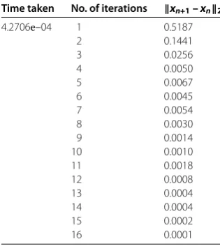
Time taken No. of iterations xn+1– xn2
4.2706e–04 1 0.5187
2 0.1441
3 0.0256
4 0.0050
5 0.0067
6 0.0045
7 0.0054
8 0.0030
9 0.0014
10 0.0010
11 0.0018
12 0.0008
13 0.0004
14 0.0004
15 0.0002
16 0.0001
Our iterative scheme (.) then becomes
yn=xn–μnAT(I–PQ)Axn,
xn+=αnr(xn) + ( –αn)PCyn, n≥.
(.)
Letr(x) =(x,x,x),x= (x,x,x). We consider initial values for the problem considered
in this example.
Case I: Takex= (., ., .). The numerical result of this problem using our algorithm
(.) with this initial value is listed in Table and the graph is given in Figure .
Case II: Takex= (., ., .). The numerical result of this problem using our
Figure 2 Example 5.1, Case II.
Table 3 Example 5.1, Case III
Time taken No. of iterations xn+1– xn2
3.2844e–04 1 0.7133
2 0.1982
3 0.0352
4 0.0069
5 0.0082
6 0.0060
7 0.0123
8 0.0025
9 0.0007
10 0.0010
11 0.0003
12 0.0002
Figure 3 Example 5.1, Case III.
Case III: Takex= (., ., .). The numerical result of this problem using our
al-gorithm (.) with this initial value is listed in Table and the graph is given in Figure .
Competing interests
The authors declare that there is no conflict of interests regarding this manuscript.
Authors’ contributions
All authors contributed equally to the writing of this paper. All authors read and approved the final manuscript.
Author details
Acknowledgements
This work was supported by the NSF of China (No. 11401063) and Natural Science Foundation of Chongqing (cstc2014jcyjA00016).
Received: 18 December 2014 Accepted: 2 July 2015
References
1. Censor, Y, Elfving, T: A multiprojection algorithm using Bregman projections in a product space. Numer. Algorithms
8(2-4), 221-239 (1994)
2. Byrne, C: Iterative oblique projection onto convex sets and the split feasibility problem. Inverse Probl.18(2), 441-453 (2002)
3. Byrne, C: A unified treatment of some iterative algorithms in signal processing and image reconstruction. Inverse Probl.20(1), 103-120 (2004)
4. Maingé, PE: The viscosity approximation process for quasi-nonexpansive mappings in Hilbert spaces. Comput. Math. Appl.59(1), 74-79 (2010)
5. Qu, B, Xiu, N: A note on the CQ algorithm for the split feasibility problem. Inverse Probl.21(5), 1655-1665 (2005) 6. Xu, H-K: A variable Krasnosel’skii-Mann algorithm and the multiple-set split feasibility problem. Inverse Probl.22(6),
2021-2034 (2006)
7. Yang, Q: The relaxed CQ algorithm solving the split feasibility problem. Inverse Probl.20(4), 1261-1266 (2004) 8. Yang, Q, Zhao, J: Generalized KM theorems and their applications. Inverse Probl.22(3), 833-844 (2006)
9. Yao, Y, Jigang, W, Liou, Y-C: Regularized methods for the split feasibility problem. Abstr. Appl. Anal.2012, Article ID 140679 (2012)
10. Ansari, QH, Rehan, A: Split feasibility and fixed point problems. In: Ansari, QH (ed.) Nonlinear Analysis: Approximation Theory, Optimization and Applications, pp. 281-322. Springer, New York (2014)
11. Xu, H-K: Iterative methods for the split feasibility problem in infinite-dimensional Hilbert spaces. Inverse Probl.26(10), Article ID 105018 (2010)
12. Yao, Y, Chen, R, Liou, Y-C: A unified implicit algorithm for solving the triple-hierarchical constrained optimization problem. Math. Comput. Model.55(3-4), 1506-1515 (2012)
13. Yao, Y, Cho, Y-J, Liou, Y-C: Hierarchical convergence of an implicit double-net algorithm for nonexpansive semigroups and variational inequalities. Fixed Point Theory Appl.2011, Article ID 101 (2011)
14. Yao, Y, Liou, Y-C, Kang, SM: Two-step projection methods for a system of variational inequality problems in Banach spaces. J. Glob. Optim.55(4), 801-811 (2013)
15. Zhao, J, Yang, Q: Several solution methods for the split feasibility problem. Inverse Probl.21(5), 1791-1799 (2005) 16. Rockafellar, RT, Wets, R: Variational Analysis. Springer, Berlin (1988)
17. Lopez, G, Martin-Marquez, V, Wang, F, Xu, H-K: Solving the split feasibility problem without prior knowledge of matrix norms. Inverse Probl.28, Article ID 085004 (2012)
18. Moudafi, A, Thakur, BS: Solving proximal split feasibility problems without prior knowledge of operator norms. Optim. Lett.8, 2099-2110 (2014). doi:10.1007/s11590-013-0708-4
19. Luke, DR, Burke, JV, Lyon, RG: Optical wavefront reconstruction: theory and numerical methods. SIAM Rev.44, 169-224 (2002)
20. Hundal, H: An alternating projection that does not converge in norm. Nonlinear Anal.57, 35-61 (2004) 21. Bauschke, HH, Burke, JV, Deutsch, FR, Hundal, HS, Vanderwerff, JD: A new proximal point iteration that converges
weakly but not in norm. Proc. Am. Math. Soc.133, 1829-1835 (2005)
22. Bauschke, HH, Matouskova, E, Reich, S: Projections and proximal point methods: convergence results and counterexamples. Nonlinear Anal.56, 715-738 (2004)
23. Matouskova, E, Reich, S: The Hundal example revisited. J. Nonlinear Convex Anal.4, 411-427 (2003)
24. Shehu, Y: Approximation of common solutions to proximal split feasibility problems and fixed point problems. Fixed Point Theory (accepted)
25. Shehu, Y: Iterative methods for convex proximal split feasibility problems and fixed point problems. Afr. Math. (2015). doi:10.1007/s13370-015-0344-5
26. Shehu, Y, Ogbuisi, FU: Convergence analysis for proximal split feasibility problems and fixed point problems. J. Appl. Math. Comput.48, 221-239 (2015)
27. Xu, H-K: Iterative algorithm for nonlinear operators. J. Lond. Math. Soc.66(2), 1-17 (2002)
28. Luke, DR: Finding best approximation pairs relative to a convex and prox-regular set in Hilbert space. SIAM J. Optim.
19(2), 714-729 (2008)