Protein-dependent prediction of messenger RNA binding using Support Vector Machines

(1)

PhD Dissertation

International Doctorate School in Information and Communication Technologies

DISI - University of Trento

Protein-dependent prediction of

messenger RNA binding using Support Vector

Machines

Carmen Maria Livi

Advisor:

Prof. Enrico Blanzieri

University of Trento

(2)

(3)

Abstract

RNA-binding proteins interact specifically with RNA strands to regulate important cellular processes. Knowing the binding partners of a protein is a crucial issue in biology and it is essential to understand the protein function and its involvement in diseases. The identification of the interactions is currently resolvable only through in vivo and in vitro experiments which may not detect all binding partners. Computational methods which capture the protein-dependent nature of the binding phenomena could help to predict, in silico, the binding and could be resistant against experimental biases.

This thesis addresses the creation of models based on support vector machines and trained on experimental data. The goal is the identification of RNAs which bind specifically to a regula-tory protein. Starting from a case study, done with protein CELF1, we extend our approach and propose three methods to predict whether an RNA strand can be bound by a particular RNA-binding protein. The methods use support vector machines and different features based on the sequence (method Oli), the motif score (method OliMo) and the secondary structure (method OliMoSS). We apply them to different experimentally-derived datasets and compare the predictions with two methods: RNAcontext and RPISeq. Oli outperforms OliMoSS and RPISeq affirming our protein specific prediction and suggesting that oligo frequencies are good discriminative features. Oli and RNAcontext are the most competitive methods in terms of AUC. A Precision-Recall analysis reveals a better performance for Oli. On a second experimen-tal dataset, where negative binding information is available, Oli outperforms RNAcontext with a precision of 0.73 vs. 0.59. Our experiments show that features based on primary sequence in-formation are highly discriminative to predict the binding between protein and RNA. Sequence motifs can improve the prediction only for some RNA-binding proteins. Finally, we can con-clude that experimental data on RNA-binding can be effectively used to train protein-specific models for in silico predictions.

Keywords

(4)

(5)

A Oma, e a me :)

(6)

(7)

Acknowledgements

First of all I would like to thank my advisor Prof. Enrico Blanzieri for his supervision and his guide through my PhD activity. Special thanks go to Yann Audic and Luc Paillard of the Institut Génétique et Développement de Rennes (France) for the internship opportunity and for giving me access to their dataset. Moreover their suggestions regarding CELF1-binding and high-throughput methods gave the right hint for my research. I am grateful to Dr. Michela A. Denti and Dr. Francesca Demichelis for their help when I was lost in biology. My sincere thanks also to Nicola Segata who taught me a lot at the beginning and for his support at the ending phase of my PhD work.

Ich danke meiner ganzen Familie f¨ur Ihre Unterst¨utzung, ganz besonders Mami und Tati, meiner Schwester Marion und meiner lieben Oma ... auf das klein Emma vielleicht auch einmal eine These schreibt.

Alla fine vorrei ringraziare una persona che era sempre al mio fianco, che ha sopportato i miei drammi personali quando tutto andava storto e che mi ha spinto quando non volevo pi`u. Purtroppo le nostre strade si sono divise ma senza di te Paolo non sarei la persona che sono oggi, alla fine di questo PhD.

Carmen

(8)

(9)

List of Tables

2.1 Physical-chemical amino acid properties . . . 9

2.2 Methods for RNA-binding site predictions . . . 17

3.1 Dataset description . . . 29

3.2 Performance of five different feature combinations . . . 32

3.3 Predicted binding and non-binding residues in six complexes using SVM1.4 . . 33

3.4 Constructed versus real RNA-strands . . . 34

4.1 Summary of the CELF1 datasets . . . 38

4.2 Performance of the CELF1 model with different feature combinations . . . 41

4.3 Results of the first experiment . . . 41

4.4 Results of the second experiment . . . 42

5.1 Performance ofOli, OliMo,OliMoSS,RNAcontext and RPISeq on the AURA-dataset . . . 50

5.2 p-values of the Wilcoxon signed-rank test forOli,OliMo,OliMoSS,RNAcontext and RPISeq. . . 51

5.3 Precision values for Oli,OliMo,OliMoSS, RNAcontext and RPISeq. . . 52

5.4 Performance of Oli, OliMo,OliMoSS,RNAcontext and bothRPISeq methods on PUM2+ in combination with two different negative datasets . . . 63

5.5 Additional analysis to test the ability of the model to identify binding sequences among general 3’UTRs. . . 64

(12)

(13)

List of Figures

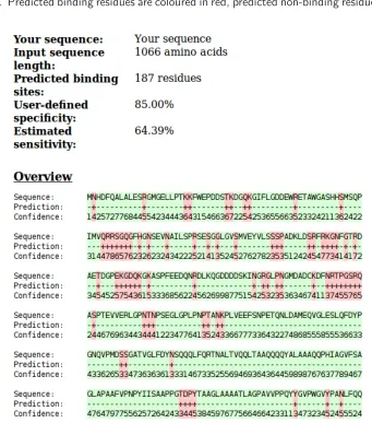
2.1 BindN+ output example for the protein sequence PUM2 HUMAN (Q8TB72). 15

3.1 RNA-sequence construction based on predicted binding residues. . . 29

4.1 CELF1-binding motif of length 11. The corresponding PSSM produces scores which are used as features in our model . . . 37

4.2 CELF1-binding motif of length 15 . . . 37

4.3 Schematic diagram of oligo feature extraction . . . 39

4.4 Schematic diagram of the motif-score calculation. . . 39

5.1 Precision-Recall curves forOli andRNAcontexton protein SLBP, MSI1, TIAL1, CEPB4, AGO2 and CPEB1. . . 53

5.2 Precision-Recall curves forOli andRNAcontext on protein CUGBP1, TNRC6A, PUM1, TNRC6C, PABP and U2AF65. . . 54

5.3 Precision-Recall curves forOli andRNAcontext on protein AGO4, QKI, TNRC6B, ELAVL1, AUF1 and AGO1. . . 55

5.4 ROC curves for Oli and RNAcontext on protein SLBP, MSI1, TIAL1, CEPB4, AGO2 and CPEB1.. . . 56

5.5 ROC curves for Oli and RNAcontext on RBP CUGBP1, TNRC6A, PUM1, TNRC6C, PABP and U2AF65. . . 57

5.6 ROC curves forOli and RNAcontext on RBP AGO4, QKI, TNRC6B, ELAVL1, AUF1 and AGO1. . . 58

5.7 ROC curve of the Oli performance on the AURAdataset. . . 60

5.8 ROC curves of Oli, OliMo,OliMoSS, RNAcontext,RPISeq-SVM and RPISeq-RF on 3K- . . . 61

5.9 ROC curves of Oli, OliMo,OliMoSS, RNAcontext,RPISeq-SVM and RPISeq-RF on PUM2- . . . 62

5.10 PR curve of Oli on PUM2+ in combination with 3K- and PUM2-.. . . 63

5.11 Precision-Recall curves for Oli and RNAcontext. . . 65

5.12 The approach . . . 66

(14)

(15)

Chapter 1

Introduction

Proteprotein and RNA-protein interactions are crucial mechanisms in cells as they are in-volved in many processes like the regulation of gene transcription or the regulation of molecular pathways. A deeper understanding of the specificity of the binding is a basic step towards the construction of computational models for simulations and in silico binding predictions.

1.1

The context

Inside the eukaryotic nucleus genes are transcribed into ribonucleic acids (RNAs). An RNA is a consecutive sequence of four nucleotides: Adenine (A), Guanine (G), Cytosine (C) and Uracil (U). There exists several types of RNAs: mRNA codifies for a protein and tRNA is involved in the translation of mRNAs into protein sequences. Proteins are organic structures made of amino acids which fold into a globular and compact form. In eukaryotic cells proteins functionally act as enzymes, structural proteins or attend to the cell signalling.

(16)

The interplay between RBPs and RNA is a fine-tuned system in the cell and its perturbation can cause disorders. Many abnormal splicing proteins are found in tumours. Therefore knowing more about RBP-RNA binding for splicing and transcription factors is of interest in cancer research. Consequently a better understanding of such interactions could help to explore their importance in diseases (Khalil and Rinn, 2011; Zhang and Darnell, 2011). Moreover, the identification of RNA targets is of special interest in biology and essential to understand proteins function (Uren et al., 2011; Auweter et al., 2006; Lichtarge and Sowa, 2002). More precise binding descriptions and accurate binding predictions are therefore needed (Mukherjee et al., 2011).

In the last decade different computational approaches focused on the prediction of RBP-RNA interactions. One category of approaches relies on the use of machine learning techniques like Neural Networks (Jeong et al., 2004), Random Forest (RF) (Liu et al., 2010), Na¨ıve Bayes (Terribilini et al., 2006) and Support Vector Machines (SVM) (Wang and Brown, 2006; Cheng et al., 2008;Wang et al., 2011) to predict single amino acids that on the protein surface potentially interact with ribonucleotides. These methods are based on the binding informa-tion extracted from 3-dimensional binding complexes and exhibit high predicinforma-tion accuracies. Unfortunately they do not consider the RNA-binding partner and give no information about the RNA sequence potentially bound by an RBP. RPISeq (Muppirala et al., 2011) instead addresses this binding-partner problem and predicts if a given RNA sequence is bound by a specific RBP, obtaining high positive-prediction rates. Another class of computational ap-proaches is that of motif-finding tools which search for binding sites on RNA strands (Glisovic et al., 2008; Lichtarge and Sowa, 2002). These methods need experimental data to extract significant sequence motifs within the bound sequences (Bailey et al., 2009) or to search for significant sequences and structural motifs by learning from both bound and non-bound data (Kazan et al., 2010). Another category of studies concentrate on the amino acid propensity (Jeong et al., 2003; P´erez-Cano and Fern´andez-Recio, 2010; Gupta and Gribskov, 2011) and the structural analysis (Bahadur et al., 2008; Jones et al., 2001) of RNA-protein complexes concluding that amino acids and nucleotides have no significant preference for binding.

(17)

The problem 3

1.2

The problem

Currently the detection of RNA targets and the identification of real binding sites has to be done through in vitro and in vivo experiments like for example the systematic evolution of ligands by exponential enrichment (SELEX) technique (Tuerk and Gold, 1990) or cross-linking and immunoprecipitation (CLIP) techniques (Kishore et al., 2011;Hafner et al., 2010; Jaskiewicz et al., 2012). Unfortunately they are costly and time consuming and each such technique has its assumptions and its limitations due to experimental biases (Kishore et al., 2011;Ank¨o and Neugebauer, 2012¨ ;Puton et al., 2011). Furthermore the assessed RBP-RNA interactions are limited to the deployed species, the deployed cell type and the experimental conditions. Moreover the observed binding sequences are restricted to the currently transcribed genes and not all binding-partners might be detected. The same holds for the non-binding information: the transcriptome in a specific sample does not cover all the possible transcripts even in the same species. Therefore by performing one experiment one may have only a subset of all possible binding and non-binding sequences.

Computational methods, capable to capture the specific and protein-dependent nature of the binding phenomena, could help to detect the interaction partnersin silicoand could be resistant against introduced biases. On the other hand high-throughput datasets contain precious information on detected RNA-protein interactions. Exploiting the information contained in these experimental data to predict in silico the other RNA-protein bindings seems therefore a promising strategy.

(18)

1.3

Our approach

Knowledge about the binding partners is of great interest in molecular biology. Computational predictions could reduce the number of laboratory experiments, which are costly and time intensive, and the lack of literature in this domain let us conclude that there is a niche which is not yet occupied. Therefore in this thesis we aim to create an in silico binding prediction based on SVM. Experimental in vivo data constitute a precious source for model constructions because they may contain important information regarding RBP affinities and binding preferences. Consequently we create our models on this kind of data. Since each RBP interacts differently with its target RNAs (Glisovic et al., 2008), it seems reasonable to train one SVM per RBP to model the specific binding phenomena. We represent each RNA sequence initially by its oligonucleotide composition and include significant binding patterns as features. Afterwards we extend the model with secondary structure and accessibility features and apply it to more experimentally derived RBPs. The use of SVMs is motivated by the good classification performance shown in previously published studies (Wang et al., 2010; Tong et al., 2008;Wang et al., 2011).

In this thesis we present a method which predicts RNA-target sequences in a protein specific way. The innovative aspect of our approach is the use of experimental datasets of detected RBP-RNA binding partners to construct prediction models. Another innovative property is the application of secondary structure and accessibility information as features. Even if our contribution to the literature is a first step, the treated argument is of importance in biology and still far away from being resolved (Puton et al., 2011). Therefore in the thesis we will show that:

• negative data, even if not detected in laboratory can be used to train models;

• secondary structure information appears to be not necessary to predict the binding;

• high-throughput data can effectively be used to create models.

1.4

Structure of the thesis

(19)

Structure of the thesis 5

(20)

(21)

Chapter 2

Background

In this chapter we introduce the RNA-protein binding first from a biological point of view by describing RNA, protein, their binding and the involved physical and chemical forces. Then we explain relevantin vivo andin vitro experiments used to detect an occurred binding. From the computational point of view this chapter introduces the state-of-the-art literature concerned with RNA-protein binding and presents some databases where biological data is stored.

2.1

RNA-protein binding. A biological point of view

Post-transcriptional regulations like alternative splicing or RNA translation are crucial processes in cells and are mediated by RBPs and transacting RNAs. Furthermore RBPs are part of complex regulatory networks and their interplay with RNA sequences is crucial in cells whereas perturbations can cause disorders (Glisovic et al., 2008; Hogan et al., 2008). Consequently a better understanding of their interactions helps to explore their importance in diseases (Khalil and Rinn, 2011; Zhang and Darnell, 2011).

It is known that RBPs interact specifically with their mRNA targets and understanding the exact molecular recognition (Westhof and Fritsch, 2011) is important to determine the mecha-nism of these specific binding. The identification of the binding partners is important in biology to determine a protein function (Uren et al., 2011; Auweter et al., 2006) and consequently better descriptions of the binding are required (Mukherjee et al., 2011).

2.1.1 RNA

(22)

have all different assignments, for example mRNAs codify for proteins. An mRNA contains several regions:

- the coding region

- the 5’ untranslated region (5’UTR) - the 3’ untranslated region (3’UTR)

The coding region of the mRNA strand is used as a kind of “blueprint” and translated into a protein sequence. Especially on the 3’UTR several regulatory sequences and RBP binding sites are established (Cor`a et al., 2007; Hogan et al., 2008). Usually RNA strands appear single stranded but guided by molecular forces, such as hydrogen bonds and stacking interactions, some RNAs can form secondary structures like stems, hairpin-loops and bulges.

There exists in silico methods which predict the formed secondary structure of an input se-quence. For instance the Vienna RNA package (Lorenz et al., 2011) provides software tools to predict RNA secondary structures, to analyse and to compare them. The predictions use different approaches based on the minimum free energy, on the pair probabilities or based on suboptimal structure folding. For instance RNAfold calculates the minimum free energy secondary structure of a corresponding RNA (Hofacker et al., 1994).

2.1.2 Protein

An mRNA sequence codifies for a protein sequence. Proteins are organic structures build up by a consecutive sequence of amino acids, also called the primary structure of the protein. 20 amino acids exist in nature. Table 2.1 lists the 20 amino acids and some of their molecular properties. Similarly to RNA also the protein sequence forms secondary structures and folds into a 3-dimensional structure. Small molecular forces like hydrogenbonds, Van der Waals forces, stacking interactions and electrostatic interactions (Auweter et al., 2006) induce the formation of three types of secondary structures called α-helix, β-sheets and coils. The ar-rangement of these structures in the 3-dimensional space is called the tertiary structure in which the protein folds into a compact and globular form. Each element of the protein chain, namely each amino acid, has individual chemical and physical properties such as charge, molec-ular mass or hydrophobicity. These properties determine the folding of the protein and are involved in the destined function of the folded protein.

2.1.3 The binding

(23)

RNA-protein binding. A biological point of view 9

Table 2.1: Physical-chemical amino acid properties. The Table lists each amino acid by name and gives some values regarding its hydrophobicity (Kyte and Doolittle, 1982), its molecular weight (Artimo et al., 2012) and the acid dissociation constant pKa for each side-chain (Parrill, 1997).

Name Hydrophobicity Chemical structure Molecular weight pKa1a

pKa1b

[g/mol]

Alanine 1.8 C3H5ON 71.0788 2.35 9.87

Arginine -4.5 C6H12ON4 156.1875 2.01 9.04

Asparagine -3.5 C4H6O2N2 114.1038 2.02 8.80

Aspartic Acid 3.5 C4H5O3N 115.0886 2.10 9.82

Cysteine 2.5 C3H5ONS 103.1388 2.05 10.25

Glutamic Acid -3.5 C5H7O3N 129.1155 2.10 9.47

Glutamine -3.5 C5H8O2N2 128.1307 2.17 9.13

Glycine -0.4 C2H3ON 57.0519 2.35 9.78

Histidine -3.2 C6H7ON3 137.1411 1.77 9.18

Isoleucine 4.5 C6H11ON 113.1594 2.32 9.76

Leucine 3.8 C6H11ON 113.1594 2.33 9.74

Lysine -3.9 C6H12ON2 128.1741 2.18 8.95

Methionine 1.9 C5H9ONS 131.1926 2.28 9.21

Phenylalanine 2.8 C9H9ON 147.1766 2.58 9.24

Proline -1.6 C5H7ON 97.1167 2.00 10.60

Serine -0.8 C3H5O2N 87.0782 2.21 9.15

Threonine -0.7 C4H7O2N 101.1051 2.09 9.10

Tryptophan -0.9 C11H10ON2 186.2132 2.38 9.39

Tyrosine -1.3 C9H9O2N 163.1760 2.20 9.11

Valine 4.2 C5H9ON 99.1326 2.29 9.72

1

the pKa is defined as the logarithm of the dissociation constant Ka[mol/L]: pKa = −log₁₀(Ka)

a

pKa of the carboxylic-acid group

b

(24)

1998;Cl´ery et al., 2008). After the analysis of several RNA-protein complexes Draper (Draper, 1999) confirms that some proteins recognize a specific sequence of ribonucleotides whereas other proteins “bind to RNA hairpins and loops” (Guzman et al., 1998).

- Some RBPs use so-called binding motifs to dock RNA. Binding motifs are specialised do-mains arranged on the protein surface and able to bind ribonucleotides. Many scientific works address the analysis of the domain specific binding. The most studied domains are probably the RNA recognition motif (RRM), the K-Homology (KH) domain, the Zinc binding domain, the double stranded RNA-binding domain (dsRBD) and the Pumilio ho-mology domain (PUF or PUM-HD) (Glisovic et al., 2008; Auweter et al., 2006;Guzman et al., 1998;Draper, 1999; Cl´ery et al., 2008).

- Other RBPs, independently from the presence or from the absence of binding domains on the protein surface, bind specific sequences on the target RNA, called sequence motifs or consensus sequences (Ray et al., 2009). Some proteins can bind also structural motifs of the RNA sequence such as bulges or stem-loops (Jones et al., 2001; Draper, 1999; Kishore et al., 2010).

- Yet other RBPs use for binding neither motifs on the protein surface nor motifs on the target RNA: they dock to the RNA backbone phosphate or ribose group (Guzman et al., 1998; Draper, 1999).

The forces guiding the binding are similar to the forces which lead to the formation of the secondary and the tertiary structure of the protein. The binding is directed by several fac-tors including hydrogen bonds, base-stacking, electrostatic and hydrophobic interactions be-tween amino acids and ribonucleotides (Guzman et al., 1998; Draper, 1999; P´erez-Cano and Fern´andez-Recio, 2010; Jones et al., 2001; Auweter et al., 2006) . Also the 3-dimensional structure of the protein and its binding-pocket influences the binding: the “mutual accommo-dation of the protein and RNA-binding surfaces” (Draper, 1999) determines significantly the ligation (Auweter et al., 2006). The RNA can insert itself spatially and “. . . the side chains of the protein have to access the edges of the RNA bases” (Westhof and Fritsch, 2011).

(25)

RNA-protein binding. A biological point of view 11

2.1.4 Laboratory experiments

Different in vivo and in vitro experimental techniques are used in biology to detect RBP-binding targets (Glisovic et al., 2008). In vivo high-throughput techniques are able to identify binding interactions genome-wide and to observe the binding in the living cell. However each of these techniques has its strength and its weakness regarding experimental errors (Corden, 2010; Ank¨o and Neugebauer, 2012¨ ;Khalil and Rinn, 2011).

Systematic Evolution of Ligands by Exponential Enrichment (SELEX)

SELEX is anin vitromethod whose goal is to identify the nucleic acid (DNA or RNA) sequences bound by an RBP of interest. Out of a pool of artificially generated RNA sequences the technique detects high-affinity targets. Kishore and colleagues (Kishore et al., 2010) argue that this high-affinity is not always the most specific one and Jeffry L. Corden (Corden, 2010) affirms that “. . . such short sequences have limited value in predicting in vivo binding sites”. However a frequent application of SELEX is the detection of a consensus sequence in the experimental outcomes by searching for significant motifs. Several motif based sequence analysis tools implement algorithms which discover motifs in these sequences and calculate the corresponding position-specific scoring matrices (PSSM) (for a more detailed description see Section2.2.3).

Cross-linking and immunoprecipitation assay (CLIP)

Thein vivodetection of RBP-RNA interactions can be done by the “fixation”, also called cross-linking, of the occurred binding in the living cell using UV light. After the cross-linking the cell is broken and the interacting elements are isolated. This technique is called Cross-linking and immunoprecipitation assay (CLIP). The obtained pieces of transcripts can be analysed via high-throughput sequencing and is than calledHITS-CLIP (high-throughput sequencing CLIP) (Zhang and Darnell, 2011). An advancement of the CLIP technique is Photoactivatable-ribonucleoside-enhanced cross-linking and immunoprecipitation (PAR-CLIP) which facilitates the cross-linking and results in a much higher number of detected binding couples (Hafner et al., 2010). The advantage of these techniques is the detection of “real” binding in living cells and it is genome-wide. On the other hand it has been shown that certain RBPs are active only during specific cellular life-cycles (Hogan et al., 2008). Hence the binding is limited to the current cell stage, the currently transcribed genes and the tissue. Thereforein vivo techniques may not be able to catch all possible targets (Ank¨o and Neugebauer, 2012¨ ).

(26)

RNA-protein interaction maps. Also Piranha (Uren et al., 2012) detects genome-wide binding sites based from CLIP data.

2.2

RNA-protein binding. A computational point of view

“How proteins selectively bind specific sites on nucleic acids has been a challenging and in-teresting problem since the earliest days of molecular biology” (Draper, 1999). Therefore extensive studies on protein-protein and on DNA-protein interactions have been done in the past and only a decade later RNA-binding sites on proteins have been studied and have been dissected. These investigations revealed the diverse nature of RNA-binding sites compared to the well-studied DNA-binding sites.

In this section we review different computational attempts which study and predict RNA-RBP interactions:

- analysis of the binding site and the binding-interaction (Section 2.2.1): dissection and statistical analysis of the 3-dimensional binding complex to study the interaction mech-anism and the binding preferences for each amino acid or the involved forces;

- prediction of single elements on the protein surface able to bind ribonucleotides (Sec-tion 2.2.2): machine learning techniques like Random Forest Method, Support Vector Machines or Neural Networks are applied to predict for each amino acid in a protein sequence if it binds to a ribonucleotide or not;

- tools to search significant patterns in the sequences i.e. binding motifs (Section 2.2.3);

- molecular recognition and docking simulations: these simulations are used to predict the RNA-protein binding based on structural information, free energy calculations, RNA plasticity and hydrogen-bonds. These approaches will not be addressed as they are beyond the scope of this thesis.

2.2.1 Dissection and analysis of RNA-protein complexes

(27)

RNA-protein binding. A computational point of view 13

database for Protein-nucleic Acid (BIPA)(Lee and Blundell, 2009) just asNPIDB (database of nucleic acids-protein interactions) (Spirin et al., 2007) provide information about size, shape, residue propensity, secondary structure composition, domain and intermolecular interactions of the binding sites.

Statistical analysis of the 3-dimensional binding complexes revealed that even if there is no significant tendency of a residue to bind a specific ribonucleotide some combinations are preferred (Terribilini et al., 2006). Exploring amino acid propensities, secondary structure motifs and atom-atom contacts shows that Arginine and Lysine seem to be favoured within protein binding sites and van der Waals interactions seem much more frequent than hydrogen bonds (Jones et al., 2001; Bahadur et al., 2008;Morozova et al., 2006; Gupta and Gribskov, 2011; Pancaldi and Bähler, 2011). Considering the general negative charge of the RNA sequence, a tendency to find positively charged amino acids in the binding pocket was expected. Indeed Arginine and Lysine are positively charged amino acids. Different numbers are reported in literature regarding the interactions of amino acids: Hoffman et. al. (Hoffman et al., 2004) notes that in 23% of the cases residues bind to ribonucleotides ribose, 51% to the phosphate and only 26% to the base. This tendency is confirmed by other studies too (Morozova et al., 2006; Bahadur et al., 2008;Ellis et al., 2007; Pérez-Cano and Fernández-Recio, 2010; Gupta and Gribskov, 2011).

Analysis of hydrogen bonds (Jeong et al., 2003; Kim et al., 2003), secondary structure inter-actions (Jones et al., 2001), backbone contacts (Bahadur et al., 2008; Gupta and Gribskov, 2011), steric exclusions and binding pocket shapes (Morozova et al., 2006; Shazman et al., 2011) try to determine the mechanism of the binding interaction. And in fact protein atoms are able to form a dense binding pocket around the ribonucleotide to create a complementary shape between base and pocket. Also the stacking interactions seem to be determinant for RNA recognition (Morozova et al., 2006). Other investigations address the specific interaction of ribosomal proteins (Ciriello et al., 2010) and the difference between the binding pockets regarding the bound RNA-type (Ellis et al., 2007;Bahadur et al., 2008).

2.2.2 Binding residue prediction

(28)

this way a dataset with binding and non-binding residues is constructed and represents the positive and the negative examples to train classifiers.

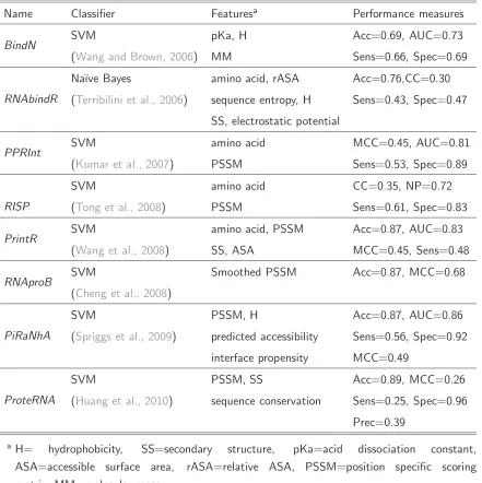
Table 2.2 shows an overview of previously published works reporting their performance, the classifier and the used features. The aim of the table is to list the works and not to compare them. In particular the reported performance measures have no comparative function as the single classifiers are trained on different datasets and apply different validation procedures, for instance a 5-,10-, or 7-fold cross or leave-one-out validations.

Wang and Brown (Wang and Brown, 2006) propose an SVM-based approach, called BindN, which takes as input the protein sequence. Each amino acid is described by three biochemical features: the acid dissociation constant value (pKa) of the side chain, the hydrophobicity (H) index and the molecular mass (MM). The pKa specifies the acidity of an amino acid. Weak acids have a pKa value in range of -2 to 12, whereas a pKa value smaller than -2 is said to be a strong acid. The hydrophobicity is a chemical property and means the rejection against water molecules. Hydrophobic elements tend to avoid the contact with water. Then a model is trained with several sequence instances, where an instance represents a subsequence of a certain lengthw. From a protein sequence withnamino acid residues a total of(n−w−1)data instances can be extracted using a sliding window technique. The target residue is positioned in the middle of the window and (n−w−1)

2 neighbour-residues on each side provide additional

information. The target residue is labelled as positive when it is defined as “binding” otherwise it is labelled as negative. This sliding window technique is used in all methods to extract several data instances from the input sequence. BindN performs with a specificity of 0.69, a sensitivity of 0.66 and an accuracy of 0.69. An extended version, called BindN+ (Wang et al., 2010), adds evolutionary information in form of position-specific scoring matrices (PSSMs) and uses the mean and the standard deviation of the three biochemical features introduced before. Combining these features results in an increased performance. Figure 2.1 shows an example output of BindN+.

(29)

(30)

0.53. Similar feature combinations are applied in RISP(Tong et al., 2008), RRINTR (Wang et al., 2008) orProteRNA(Huang et al., 2010). PSSM profiles which incorporate evolutionary information are a common features not only in the prediction of RNA-protein interactions, but also in the prediction of DNA-protein and protein-protein interactions. RNAProB(Cheng et al., 2008) went a step further and adopted a “smoothed PSSM”, created on a traditional PSSM profile and considering the PSSM neighbourhood of the target residue. The performance of the classifier applied on three different benchmark datasets is rather high with an average specificity of 0.88 and an average sensitivity of 0.74.

Each amino acid has its own physical and chemical characteristics (see Section 2.1.2) repre-sented by properties like hydrophobicity or molecular mass, which may determine its ability to be involved in binding or not. Therefore it can be more likely to find specific residues in the binding site then elsewhere. Following this reasoning PiRaNhA(Spriggs et al., 2009) adds the interface propensity (IP) to its features. A similar approach is integrated also in PRNA (Liu et al., 2010) which uses a Random Forest (RF) classifier. The residues are encoded, besides other features, as interaction propensities extended to three amino acids. Taking into account also the nearest neighbourhood of the considered residue the IP is calculated on triplets in-stead on single residues. Subtracting one descriptor after another the feature importance can be evaluated. The triplet IP and structural features like accessible surface area (ASA) and secondary structures turned out to be the most powerful features in PRNA.

More sophisticated approaches, instead of using the residue of interest and its sequential neighbours to investigate the binding, use surface patches and clefts which surround the target residue. Patches and clefts consider the 3-dimensionality of the binding pocket and the binding surface. In that respect a surface patch is defined as RNA-interacting if a limited amount of accessible surface residues belong to it. Whereas a binding-cleft, including cavities and grooves, contains at least 10 accessible and interacting residues (Chen and Lim, 2008). PRIP (Maetschke and Yuan, 2009) applies sequential, graph-topological and spatial information to individuate the binding patches. The application of both SVM and Na¨ıve Bayes classifier confirms that the former performs better.

(31)

Table 2.2: RNA-binding site prediction methods. The approaches attempt to predict RNA-interacting residues in protein sequences. Listed are name, classifier, applied features and some performance values: accuracy (Acc), sensitivity (Sens), specificity (Spec), area under the ROC curve (AUC), correlation coefficient (CC) and net prediction (NP). Shown is the performance of the best feature combination presented in the paper. This table is not intended for comparison.

Name Classifier Featuresa

Performance measures

BindN SVM pKa, H Acc=0.69, AUC=0.73

(Wang and Brown, 2006) MM Sens=0.66, Spec=0.69

RNAbindR

Na¨ıve Bayes amino acid, rASA Acc=0.76,CC=0.30

(Terribilini et al., 2006) sequence entropy, H Sens=0.43, Spec=0.47

SS, electrostatic potential

PPRInt SVM amino acid MCC=0.45, AUC=0.81

(Kumar et al., 2007) PSSM Sens=0.53, Spec=0.89

RISP

SVM amino acid CC=0.35, NP=0.72

(Tong et al., 2008) PSSM Sens=0.61, Spec=0.83

PrintR SVM amino acid, PSSM Acc=0.87, AUC=0.83

(Wang et al., 2008) SS, ASA MCC=0.45, Sens=0.48

RNAproB SVM Smoothed PSSM Acc=0.87, MCC=0.68

(Cheng et al., 2008)

PiRaNhA

SVM PSSM, H Acc=0.87, AUC=0.86

(Spriggs et al., 2009) predicted accessibility Sens=0.56, Spec=0.92

interface propensity MCC=0.49

ProteRNA

SVM PSSM, SS Acc=0.89, MCC=0.26

(Huang et al., 2010) sequence conservation Sens=0.25, Spec=0.96

Prec=0.39

a

(32)

Name Classifier Featuresa

BindN+

SVM PSSM Acc=0.77, AUC=0.82

(Wang et al., 2010) mean±std of pKa Sens=0.71, Spec=0.78

mean±std of H MCC=0.39

mean±std of MM

PRNA

Random forest rASA, SS, PSSM Acc=0.82, MCC=0.48

(Liu et al., 2010) pKa, H, triplet IP Sens=0.81, Spec=0.86

number of atoms

electrostatic charge

hydrogen bonds

no name

SVM Smoothing PSSM, ASA Acc=0.88, MCC=0.68

(Wang et al., 2011) pKA, H, MM Sens=0.78, Spec=0.91

hydrophobic moment

net charge index of side chain

net charge index moment

propensity

propensity moment

no name

SVM amino acid frequency, H Acc=0.90, CC=0.24

(Choi and Han, 2011) amino acid position, ASA Sens=0.60, Spec=0.91

chain length, MM, pKa NP=0.75

triplet IP, partner information

a

(33)

Many of the previous methods predict binding residues without considering the RNA-binding partner. They give no information about the RNA-sequence potentially bound by an RBP. OnlyRPISeq (Muppirala et al., 2011) addresses this issue and predicts the binding between a given RBP and its RNA-target using both SVM (RPISeq-SVM) and RF (RPISeq-RF) method. The classifiers are trained with simple sequence features using Conjoint Triad Feature (CTF) of length 3 to encode the protein and oligonucleotides (oligos) of length 4 to encode the RNA sequence. In CTF the amino acids are divided in seven different groups reducing the alphabet from 20 elements to 7 elements. A protein is encoded with 343 features by counting the (normalized) frequency of all occurring triplets. The RNA sequence is encoded similarly by counting and normalizing the frequencies of all occurring oligos of length 4. Finally each RBP-RNA pair is represented by 599 features. Two different datasets are created using interacting RNA complexes as positive examples, and randomly coupled “non-interacting” RBP-RNA pairs as negative examples. The first dataset contains mainly interactions with ribosomal proteins and ribosomal RNAs and the second dataset only non-ribosomal complexes. In a 10-fold cross validation RPISeq-RF performs better on both datasets than RPISeq-SVM. Both classifiers achieve high performance values when applied on the ribosomal-dataset with an accuracy of 0.89 and 0.87, for RF and SVM respectively. The RF-model achieves a precision of 0.89 and an AUC of 0.97, whereas the SVM applied on the ribosome dataset achieves a precision of 0.87 and an AUC of 0.92. Much lower values are reached on the second dataset without ribosomal complexes: the accuracies vary between 0.76 (RPISeq-RF) and 0.72 (RPISeq-SVM). The precision does not exceed the threshold of 0.75 and also the AUC values with 0.85 (RF) and 0.81 (SVM) are lower compared to the ribosomal-dataset.

2.2.3 Motif finding tools

Some RBPs can bind specific sequence patterns on their targets, called motifs. Motifs are patterns in RNA, DNA or protein sequences which can be modelled by position-specific scoring matrices, called PSSMs. PSSMs can be used to describe potential binding sites and are also applied to identify evolutionary similar proteins and to discover evolutionary conserved functional sites (Lichtarge and Sowa, 2002). Experimentally detected binding motifs are not always available, but there existin silico tools which search for significant patterns in a group of RNA sequences known to be bound by an RBP.

(34)

RNAcontext (Kazan et al., 2010) discovers structural motifs within related sequences. The tool searches for significant sequential and structural binding preferences in a set of target and non-target examples by using a structural context alphabet (i.e. paired, unpaired, hairpin loop) based on secondary structure predictions. Finally the model can be applied to detect the identified motif in a set of unknown sequences.

2.3

Machine learning

New high-throughput technologies and next-generation sequencing produce a huge amount of biological data. These data needs to be stored and to be searchable for biologically relevant questions. Artificial intelligence and machine learning are applied to mine, to explore, to analyse and to extract the knowledge contained in these genomic, proteomic or transcriptomic data. Hence machine learning is an important field in bioinformatics (Inza et al., 2010;Jensen and Bateman, 2011).

SVMs (Vapnik, 1995) are one of the most used supervised machine learning techniques and have been widely applied in bioinformatics (see Section2.2). The basic idea is that the classifier learns a mathematical function on input examples and classifies than new unknown examples.

2.3.1 Support vector machine (SVM)

The SVM classifier discriminates linearly between input vectors xi ∈ Rp, with p being the

number of features. The input examples i = 1,2, ..., n are associated with different classes

yi ∈ {+1,-1}: an input vector xi belongs to the positive class with label +1 or to the

negative class with label −1. The goal of a SVM is to find a discrimination function f(x)

which divides the two classes in such a way that the label for new vectors can be predicted:

f(x) = sign(< w, x > +b) where w is the weight vector, the scalar b the bias and sign

returns the sign of the argument. f(x) = 1 assigns the positive class label, otherwise the negative one.

During the training the hyperplane tries to divide the two classes linearly. This can be controlled by parameters that provide a more flexible classification of the input vectors. The “softmargin” approach introduces so-called slack variables allowing an example to be misclassified. The use of these slack variables can be regulated by the constantC >0. The SVM can map the input space into a feature space using kernel-functions. To implement the classifier we use the freely available SVM package LibSVM (Chang and Lin, 2011) and apply both the linear kernel and the RBF kernel.

(35)

Data balancing 21

FaLKM-lib (Segata, 2009) with the linear kernel.

2.4

Data balancing

A frequent problem with biological datasets is that they are unbalanced. Usually the number of negative data points is much higher than the number of positive ones (Terribilini et al., 2006; Cheng et al., 2008; Wang and Brown, 2006). Machine learning techniques learn on input examples and using highly-unbalanced datasets affects their performance. To overcome the unbalancing different approaches are proposed in literature such as several forms of data re-sampling (over-re-sampling, under-re-sampling), one-class learning or by using different class weights (Kotsiantis et al., 2006). One re-sampling method is a synthetic minority over-sampling technique called SMOTE (Chawla et al., 2002). The method amplifies the positive dataset by creating new synthetic instances and forces the classifier to become more general.

2.5

A binary classifier like the SVM assigns to predicted binding sequences the positive class label (+1) and to sequences predicted as non-binding the negative class label (−1). Correct assignments to the positive or the negative class increase the numbers of the true positives (TP) or the true negatives (TN), respectively. Wrongly attributed elements increase the false negatives (FN) or false positives (FP). Different measures can be calculated to assess the performance of a classifier. In this thesis we use:

Accuracy (Acc) is the rate of correct and false predicted elements over the total dataset

ACC = T P +T N

T P +F P +F N +T N (2.1)

A weakness of the ACC is that its value can be high even if one class is never or poorly predicted. For instance when all elements of the negative class are predicted as negatives but no positive element was assigned to the positive class.

The Matthews correlation coefficient (MCC) instead is a balanced measure and indicates the correlation between observed and predicted classification

MCC = p T P ·T N −F P ·F N

(T P +F P)·(T P +F N)·(T N +F P)·(T N+F N) (2.2)

The sensitivity

Sens= T P

(36)

measures the ability of the classifier to identify positive elements whereas the specificity

Spec= T N

T N+F P (2.4)

measures the proportion of correctly classified negative elements.

The precision (Prec), also called positive predictive value, indicates the portion of positive classified examples that are really positive:

P rec= T P

T P +F P (2.5)

The creation of the receiver operating characteristic (ROC) curve is a common way to visualize a model performance. The x-axis shows the false positive rate and the y-axis displays the true positive rate by varying a parameter, in our case the classification threshold. True positive rate and false positive rate are defined as

T P R= T P

T P +F N (2.6)

and

F P R= F P

F P +T N (2.7)

respectively. More the ROC curve advances to the upper-left corner, the better is the classifi-cation ability of the model. A curve near the diagonal characterizes a “random” classificlassifi-cation (Fawcett, 2006). A similar visualization gives the Precision-Recall (PR) curve showing the precision on the y-axis and the recall on the x-axis:

Recall = T P

T P +F N (2.8)

More the PR curve advances to the upper-right corner, the better is the prediction of the model (Davis and Goadrich, 2006). By calculating the area under the ROC curve (AUC) the performance of a classifier can be reduced to a single value. A perfect classifier has an AUC of 1.

2.6

Biological databases

In this section we describe some databases which are relevant in this thesis.

2.6.1 The University of California, Santa Cruz (UCSC) Genome Browser

(37)

Biological databases 23

and to analyse the data. The collection contains linked data regarding genes, their transcripts and protein products deriving from well-known sources like GenBank (Benson et al., 2013), Ensembl Genes (Flicek et al., 2010), RefSeq (Pruitt et al., 2007) or the UniProt Knowledgebase (UniProtKB) (Magrane et al., 2011).

2.6.2 The Ensembl project

Another collection of databases with genomic material of about 60 species (September 2011), annotations and sequence data is “The Ensembl project” (Flicek et al., 2010). Ensembl provides links to UCSC Genome Browser and integrates DNA data, genes, transcripts and information about sequence variations or regulation. Tools such as BioMart (Smedley et al., 2009) can be used to search across the databases and to perform complex queries.

2.6.3 The RCSB Protein Data Bank (PDB)

PDB (Bernstein et al., 1977) stores 3-dimensional macromolecular crystal structures obtained by nuclear magnetic resonance, X-ray crystal structure determination, cryo-electron microscopy and theoretical modelling (Berman et al., 2000). Each entry is identified by a unique acces-sion number and the file format contains the atomic coordinates for each structure. The 3-dimensional structure can be visualized by molecular viewers. Beside this other information regarding the macromolecule is stored, e.g. the sequence information, molecular functions or annotations, referencing other databases such as UniProtKB.

2.6.4 The Atlas of UTR regulatory activity (AURA)

The manually curated AURA (Dassi et al., 2012) is a database containing information about human UTRs. Currently (February 2013) it contains the binding data for 103 RBPs and more than 127000 UTRs, deriving from 63138 transcripts of about 29000 genes. The online database provides information regarding RBPs, their function and their bound 3’UTR and 5’UTR se-quences. The datasets and the binding information derive from laboratory experiments like CLIP, PAR-CLIP or SELEX. AURA can be searched in different ways: by searching directly for UTRs, by searching for UTRs bound by an RBP of interest or by using the BioMart-equivalent called AURA Mart.

(38)

(nr-database) contains non-redundant sequences from GenBank (Genbank CDS translations) together with protein sequences from Refseq, PDB and UniProtKB. The nr-database can be used to perform a Blast-search.

The Basic Local Alignment Search Tool (BLAST) (Altschul et al., 1997) has been developed at the NCBI and searches for genes and proteins in databases. The algorithm tries to find similar gene or protein sequences and queries the sequence in question against large datasets. BLAST can also be used to identify functional and evolutionary sequence information. Several types of BLAST are available: to search for a protein sequence in a protein database or to search for a protein sequence in a nucleotide database. A special way to search in databases is the use of PSI-BLAST (Position-Specific Iterated BLAST) (Altschul et al., 1997) which creates a PSSM by matching the query sequence against the database. Afterwards the PSSM can be used to search for evolutionary similar sequences.

2.6.6 The Gene Expression Omnibus (GEO)

(39)

Chapter 3

Preliminary analysis

Predicting amino acids to be involved in ribonucleotide-binding is challenging and has been ad-dressed conspicuously often (see Section2.2). Machine learning techniques like SVM, Random Forest or Na¨ıve Bayes have been trained with sequence features, like molecular mass (MM), hydrophobicity (H), the acid dissociation constant value (pKa) or secondary structures (SS); with evolutionary features, like position-specific scoring matrix (PSSM) or with 3-dimensional structure-properties, like the accessible surface area (ASA) (Wang and Brown, 2006; Kumar et al., 2007;Wang et al., 2008). These approaches do not look to the RNA sequence which can be bound by the analysed RBP but focus on the prediction of binding elements in the protein sequence. Only recently published methods involve also the RNA sequence in the binding pre-diction by using both, protein and RNA sequences (Muppirala et al., 2011) or global features like UTR characteristics or expression levels (Pancaldi and B¨ahler, 2011). Considering the predicted binding amino acid it should be possible to detect the bound RNA target-sequence. Therefore our preliminary analysis addresses the prediction of the RNA binding partner. In this Chapter we give a formal description of the binding, describe our approach and present the obtained results. Then we discuss them and conclude by outlining the next steps.

3.1

Abstraction of the binding

In order to give a precise description of the problem we define the main concepts involved in binding. The RNA is a consecutive sequence ofn nucleotides dNT P

dNT P0. . . dNT Pi. . . dNT Pn−1

The i-th nucleotide dNT Pi is composed of a base, a phosphate and a ribose sugar. There

(40)

folded sequence of m amino acids. There are 20 types of amino acids

aav ∈ {A,R,N,D,C,E,Q,G,H,I,L,K,M,F,P,S,T,W,Y,V}

withv = 1. . .20. Every amino acidaav can be described by some physical-chemical properties

prop(aav)∈ {polarity, molecular mass, hydrophobicity, pKa, charge}. The protein can form

several structures: the primary (1str), secondary (2str) and tertiary (3str) structure. To form the primary structure 1str of the protein the amino acids bind together through the so-called peptide bound. After this connection the single amino acid aav is called residue rj at the

sequence position j inside the protein chain

r0. . . rj. . . rm−1

The protein chain can form the secondary structure 2str by shaping in the secondary structures

α-helices, β-sheets or coils. Thus a secondary structure ssl∈ {α, β, coil} can be assigned to

every rj within the protein P. Suppose that aav ∈ {A, R, N, D, C...} and rj is the amino

acid aav at the j-th position in the primary structure of a protein P, than:

2strP: {A, R, N, D, C, . . .} → {α, β, coil}

2strP(rj) 7→ ssl

For our purpose it is sufficient to define the tertiary structure 3str as the transformation of the amino acid rj into a 3-dimensional space with the coordinates x,y,z:

3strP: {A, R, N, D, C . . .} → R3

3strP(rj) 7→ (x, y, z)

An interaction is a kind of physical-chemical phenomenon which occurs between two or more objects. The interaction between a nucleotide dNT Pi and a residue rj is defined asIij where

Iij ∈ {van der W aals, electrostatic interaction, hydrogen bond, base stacking}. One

type of interaction can be stronger than another. The binding is the result of an interaction and ends in a stable association and in the formation of a molecular complex. A complexC is the collectivity of all residuesrj of the proteinP and all nucleotidesdNT Pi of the RNA which

are involved in an interaction Iij between rj and dNT Pi. In this context the protein binding

is a stable association of a specific piece on the protein, called binding site, to a specific piece on the RNA strand, called RNA-target sequence. The formed structure is called protein-RNA complex where the binding site of the protein P is defined as a subset of the protein chain

r0. . . rm−1, consisting of all k residues

(41)

The Approach 27

which are involved in an interaction with the nucleotides of the target RNA. The target sequence of an RNA is defined as a subset of the RNA sequence dNT P0 . . .dNT Pn−1,

consisting of all wnucleotides

t0. . . tw−1

which are involved in an interaction with a residue. Given a target and a binding site the interaction Iij between the nucleotide ti with 0≤ i≤w−1and the binding residue bj with

0≤j ≤k−1 is denoted as

ti Iij

−→bj

Given the formed interactionsti Iij

−→bj between everyti ∈t0. . . tw−1and everybj ∈b0. . . bk−1

the binding is defined as the set of all interactions formed in the complex.

3.2

The Approach

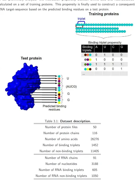
Our approach exploits a binding-residue prediction and uses the predicted elements to construct the bound RNA sequence. The bound RNA sequence is constructed by using a previously cre-ated propensity statistic. If a residue is predicted as binding we will use the propensity statistic to detect its favoured nucleotide binding partner and create the targeted RNA sequence. First we perform a simple sequence analysis on the dataset, extract all amino acid triplets which are present in the protein sequences and calculate for each its interaction propensity with ribonucleotides. In other words we detect triplets (rj−1, rj, rj+1) and check for each of

them if the target residue rj is involved in binding dNT Pi Iij

−→ rj. In such case we save the

triplet with its target residue rj and its nucleotide binding partner dNT Pi. Hence we detect

the binding preference for each triplet and construct its propensity table.

To implement the binding-residue prediction we use SVMs and apply different features. The goal is to predict the binding elements of the binding siteb0. . . bk−1 on the RBP. Evolutionary

(42)

- SVM1.1: MM, number of atoms, electrostatic charge, number of potential hydrogen-bonds and two pKa values;

- SVM1.1Beta: MM, electrostatic charge, H and two pKa values;

- SVM1.2: MM, number of atoms, electrostatic charge, number of potential hydrogen-bonds, two pKa values and ASA;

- SVM1.3: MM, number of atoms, electrostatic charge, number of potential hydrogen-bonds, two pKa values, ASA and SS;

- SVM1.4: MM, number of atoms, electrostatic charge, number of potential hydrogen-bonds, two pKa values, ASA, SS and PSSM;

The classifier with the best performance is chosen for our final approach.

The last step is the construction of the target sequence t0. . . tw−1 on the RNA which is bound

by the predicted binding-residues of the binding site b0. . . bk−1 on the RBP. Ifrj of the triplet

(rj−1, rj, rj+1) is predicted as binding we search the triplet in the propensity table and go

the way backward: dNT Pi Iij

←− rj. In this way we construct a target sequence. Figure 3.1

illustrates the described idea.

3.3

Material and Methods

3.3.1 Dataset

Our dataset is composed of 50 protein files (Terribilini et al., 2006; Kumar et al., 2007) and contains 3-dimensional RBP-RNA binding complexes downloaded from PDB (Bernstein et al., 1977), with a resolution higher than 3˚A . A pdb file can contain multiple protein and RNA chains. Therefore strands which are not involved in any kind of intermolecular interaction are eliminated. HBPLUS (McDonald and Thornton, 1994) could not resolve the structure for three files (1FJG.pdb, 1H38.pdb, 1JJ2.pdb), so they are cancelled from the dataset. Table

3.1 summarizes the properties of the dataset.

Test proteins: to carry out the test we use six randomly selected protein chains from the dataset which will not make part of the training. These are: 1A9N.pdb, 1ASZ.pdb, 1AV6.pdb, 1B7F.pdb, 1B23.pdb and 1C0A.pdb.

3.3.2 Binding Residue Identification

To identify a binding residue we check if it participates in an interaction Iij. HBPLUS is

(43)

Material and Methods 29

Figure 3.1: RNA-sequence construction based on predicted binding residues. The main idea of our preliminary analysis: the interaction propensity between amino acid and ribonucleotide is calculated on a set of training proteins. This propensity is finally used to construct a consequential RNA target-sequence based on the predicted binding residues on a test protein.

Table 3.1: Dataset description.

Number of protein files 50

Number of protein chains 116

Number of amino acids 26276

Number of binding triplets 1452

Number of non-binding triplets 11405

Number of RNA chains 91

Number of nucleotides 3188

Number of RNA binding triplets 605

(44)

The cut-off distance defines the maximal allowed distance between an interacting amino acid and a ribonucleotide. Different cut-off distances are used and vary from 2.5˚A (Kumar et al., 2007; Wang and Brown, 2006) to 5˚A (Terribilini et al., 2006). Analyses of the distribution of misclassified non-binding residues recommend a distance between 3.5˚A and 8.5˚A (Tong et al., 2008), therefore we decide to use a cut-off distance of 3.9˚A (Wang et al., 2008;Spriggs et al., 2009;Liu et al., 2010). Ribonucleotides which are spatially near an amino acid, within this cut-off distance, are labelled as binding residues otherwise as non-binding residues. We extract in total 11405 non-binding and 1452 binding residues. Running the classifier on such an unbalanced dataset caused a constant non-binding prediction for each residue. Therefore we choose randomly 1452 negative elements to adapt the number of negatives to the number of positive residues.

3.3.3 Feature Extraction and Representation PSSM

A PSSM is created by running a PSI-BLAST (Altschul et al., 1997) search against the nr-database downloaded from NCBI. With each sequence in our dataset we perform a PSI-BLAST search to obtain the PSSM of the corresponding protein.

Physical-chemical amino acid properties

Each amino acid has individual physical and chemical properties. We think that these char-acteristics strongly determine the willingness to bind. Hence we use the following features to describe each amino acid:

1. molecular mass (Table 2.1);

2. pKa of the carboxyl group (Table 2.1);

3. pKa of the amino group (Table 2.1);

4. number of atoms (Liu et al., 2010);

5. electrostatic charge (Liu et al., 2010);

6. number of potential hydrogen-bonds (Liu et al., 2010);

(45)

Results and Discussion 31

ASA

DSSP (Kabsch and Sander, 1983) is applied to calculate the ASA. The program takes as input the 3-dimensional complex and calculates the accessible area for each amino acid on the protein surface by using the atomic coordinates of the pdb file.

Secondary Structure

To extract the secondary structure of the protein, which is given in the pdb-file, DSSP is used as well. The secondary structures are divided into three groups: α-helix, β-sheet and coil. Each of them is encoded binary in a 3-dimensional vector (Wang et al., 2008) where the corresponding vector field is set to 1: for α-helix (100), forβ-sheet (010) and for coil (001). If there is no structure assigned the vector-elements are all zero (000).

Classifier Evaluation

LibSVM (Chang and Lin, 2011) package is used to construct the SVM classifier. The best parameter combination of cost C and RBF-kernel parameter γ is optimized with respect to the highest value of

(sensitivity+specif icity) 2

To evaluate our model we perform a 10-fold cross validation and calculate sensitivity, specificity and accuracy. Our dataset is strongly unbalanced with 11405 non-binding and 1452 binding residues. Therefore we balance the dataset by choosing randomly 1452 residues for each class.

3.4

Results and Discussion

(46)

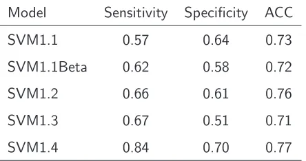
Table 3.2: Performance measures of five different feature combinations. SVM1.1: MM, number of atoms, electrostatic charge, number of potential hydrogen-bond and two pKa values.

SVM1.1Beta: MM, electrostatic charge, H and two pKa values. SVM1.2: MM, number of atoms, electrostatic charge, number of potential hydrogen-bond, two pKa values and ASA. SVM1.3: MM, number of atoms, electrostatic charge, number of potential hydrogen-bond, two pKa values, ASA and SS.SVM1.4: MM, number of atoms, electrostatic charge, number of potential hydrogen-bond, two pKa values, ASA, SS and PSSM.

Model Sensitivity Specificity ACC

SVM1.1 0.57 0.64 0.73

SVM1.1Beta 0.62 0.58 0.72

SVM1.2 0.66 0.61 0.76

SVM1.3 0.67 0.51 0.71

SVM1.4 0.84 0.70 0.77

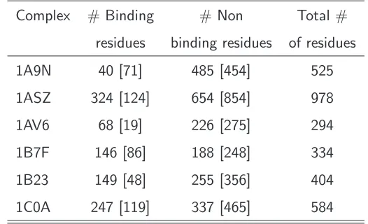
binding; for test protein 1AV6 the predicted residues are 68 whereas HBPLUS detected only 19 amino acids as binding.

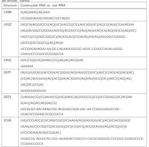
Starting from the predicted binding-triplets the RNA sequence is reconstructed using the propensity statistic. The reconstructed RNA sequence for test protein 1A9N is:

G(AG)AAAG(AG)AAA

Nucleotides in brackets can not be assigned uniquely, the binding of the investigated triplet can be with ribonucleotide A or G. The real RNA strand extracted from the corresponding pdb file is

CCUGGUAUUGCAGUACCUCCAGGU

Table 3.4 contains the reconstructed and the original RNA strands for all 6 test proteins. The final results are not satisfying which is evidenced by comparing the constructed and the real RNA strands. This insufficiency has several reasons. Without any doubt one reason is the true positive prediction of SVM1.4. Despite a high sensitivity of 0.84 in an independent 10-fold cross validation, the prediction on the test proteins shows that too many triplets are wrongly assigned to the binding class. We base our RNA-construction on these predictions so they should be more precise, which is evidently not the case when looking to the results of Table 3.3 and Table 3.4.

(47)

Conclusions 33

Table 3.3: Predicted binding residues using SVM1.4. Predicted binding and non-binding residues in six complexes. The ”real” number of binding elements extracted with HBPLUS is shown in brackets.

Complex # Binding # Non Total #

residues binding residues of residues

1A9N 40 [71] 485 [454] 525

1ASZ 324 [124] 654 [854] 978

1AV6 68 [19] 226 [275] 294

1B7F 146 [86] 188 [248] 334

1B23 149 [48] 255 [356] 404

1C0A 247 [119] 337 [465] 584

there were much more negative (11405 non-binding) than positive (1452 binding) residues. So we were constrained to create a dataset with an equal number of negative and positive elements. Also this procedure can interfere with the prediction ability of the model.

3.5

Conclusions

(48)

Table 3.4: Constructed versus real RNA-strands. Real RNA sequences bound by the correspond-ing RBP are shown in italic and constructed RNA sequences based on our binding-triplet prediction are written “normal”.

Structure Constructed RNA vs. real RNA

1A9N G(AG)AAAG(AG)AAA

CCUGGUAUUGCAGUACCUCCAGGU

1ASZ (AG)CA(AG)(UG)CU(AG)(UC)UA(CG)(CG)(AUC)GG(UC)(AG)CG(AU)(CG)A(AG)AA

(AG)(AU)GG(CG)GGGU(AUCG)(ACG)U(CG)(AG)(AU)U(AG)CA(AG)(UG)CU(AG)(UC)

UA(CG)(CG)(AUC)GG(UC)(AG)CG(AU)(CG)A(AG)AA(AG)(AU)GG(CG)GGGU

(AUCG)(ACG)U(CG)(AG)(AU)U

UCCGUGAUAGUU-AA-GG-CAGAAUGGGCGC-UGUC-CGUGCCAGAU-GGGG–

CAAUUCCCCGUCGCGGAGCCA

1AV6 UUC(CG)G(UG)AAAGC(CG)(AG)AC(ACG)UAC

GAAAAA

1B7F (AUG)UUU(AU)(ACG)GA(AC)GGUU(AG)UAU(UCG)(UC)(AUC)C(AG)(AG)(AG)(AC)

(CG)AC(AUG)UUU(AU)(ACG)GA(AC)GGUU(AG)UAU(UCG)(UC)(AUC)C(AG)(AG)

(AG)(AC)(CG)AC

GUUGUUUUUUUU

1B23 CUAUGA(CG)(CG)AUU(CG)(UG)UAUC(AG)GGG(CG)(CG)UCCGGAGC(UC)ACGAU

G(AU)(AG)AC(AG)UA(CG)

GGCGCGU-AACAAAGCGG–AUGUAGCGGA-UGC-AA-CCGUCUAGUCCGG–

CGACUCCGGAACGCGCCUCCA

1C0A (UG)CCC(AUC)C(UC)AU(CG)C(UC)AAGA(AG)GA(UG)G(AC)(AC)GC(ACG)(UG)C

GGAG(AUC)CCGU(CG)ACG(UG)(UC)(CG)UCG(ACG)U(AU)U(AG)(ACG)(UC)G

(UC)CAUAA(AU)G(CG)G(AC)

(49)

Chapter 4

RNA-binding prediction for CELF1. A

case study

The interplay between RBPs and RNAs is highly specific and crucial for cellular physiology. Identifying the RNA targets for a given RBP is important to understand its function and therefore of interest in biology. Several molecular approaches like SELEX or CLIP-seq detect RBP-RNA interactions and consequently the RBP-specificity but computational models and binding predictions would greatly reduce “hands-on” experimental time and experimental costs. On the other hand experimental data, especially from high-throughput techniques, constitute an important source and host precious information regarding the binding of the analysed RBP. Tapping the full potential of suchin vivo and in vitro datasets seems a good strategy, because the data can be used to predict in silico RNA-protein bindings.

RBPs have different ways to bind their RNAs: they can bind particular patterns on the sequence or associate secondary structures. For instance CELF1 (also known as CUGBP1 or EDENBP) is a human RNA-binding protein which binds mainly single stranded UGU-rich RNA-segments (Marquis et al., 2006; Kress et al., 2007). Being present in the nucleus and cytoplasm of the cell, CELF1 controls post-transcriptional processes at many levels.

In this chapter we propose the basic framework of our approach and apply it to CELF1. We use SVMs to classify CELF1-binding sites and to discriminate binding from non-binding RNAs. Additionally we perform two experiments which verify the prediction ability of the proposed approach. First we briefly describe the concept, the dataset and the applied features. Then we detail the experiments, the obtained results and discuss them.1

1

(50)

4.1

The Approach

The goal is to discriminate between CELF1-target RNAs and sequences which are not tar-geted by CELF1. Therefore we exploit the results of a CLIP-seq dataset and use SVMs for classification. We describe each RNA sequence with 287 features: 256 features are obtained by encoding the RNA sequence in oligonucleotides (oligos), 30 features are motif scores cal-culated by applying PSSMs and the last single feature is the presence of a UGU-rich motif in the sequence.

RBP CELF1 is known to bind single stranded RNA sequences by targeting a specific sequence pattern. Due to a previously performed SELEX experiment (Marquis et al., 2006) two similar binding motifs have been detected with MEME: Figure4.1and Figure4.2 show their sequence logo. A third and independent binding motif has been searched also within the CLIP-seq dataset (by using MEME). The motif is not shown as it changes slightly for each fold. MEME provides PSSMs which are finally used to calculate the motif-scores along each RNA strand. In our approach the presence of the binding site is described by means of these scores and they are calculated for each motif on each sequence. In other words we encode the binding site by using the ten highest scores for each motif (10×3) as features.

The binding is not only determined by the presence of a specific binding motif but can depend also on the sequence-context of the motif. To incorporate the individual sequence composition we encode each RNA strand by its oligo frequency. The appearance of each oligo in the sequence sets the corresponding feature vector field.

Based on structural information a particular UGU-rich binding motif is known to be bound by CELF1. We describe the UGU-rich binding motif by means of a binary feature which is set to

1 if the motif is present in the sequence, otherwise it is set to 0. All the described features fit the CELF1-binding specificities.

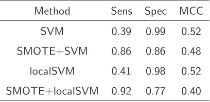
A 10-fold cross validation and two experiments are performed to validate the model. In the first experiment we apply SVM and localSVM on cluster sequences bound by CELF1 and on non-bound sequences. Additionally we attempt to balance the dataset by applying a balancing algorithm. The second experiment divides the training data in subsets. Each set contains sequences of a limited length l and validates the prediction performance on subsequences of the test data.

4.2

Material and Methods

4.2.1 Datasets

(51)

Material and Methods 37

Figure 4.1: CELF1-binding motif of length 11. Two CELF1-binding motifs have been found in a previously performed SELEX experiment. The corresponding PSSMs produce scores which are used as features in our model.

MEME (no SSC)19.7.2011 08:46

0 1 2 bits 1 G C

T

2 A T C

G

T

3C4

G

T

5

T

T6

A

G

7

T

A

G

8

T

9

GA

T

10 A CT

G

11

T

Figure 4.2: CELF1-binding motif of length 15.

MEME (no SSC)19.7.2011 08:47

0 1 2 bits 1 C

T

G

2 A

CG

T

3

C

G

T

4

T

A5

T

G

6

T

C

G

7

T

8

T

A9

CT

G

10

T

11 A

G

T

12 A

T

13

G

14

T

15

G

(52)

Table 4.1: Summary of the datasets. The positive data contains binding clusters from a CLIP-seq experiment with CELF1. The negative examples used to create the model are formed by expressed but not bound transcripts.

Dataset No. of chains Shortest/longest Average length

CLIPData 1932 29/1401 170

original NegData 36701 11/16193 952

NegData 24680 19/999 379

consists of 1932 cluster sequences identified to be bound in vivo by CELF1.

NegData The dataset is constituted of 3’UTRs from genes expressed in Hela-kyoto cells and not bound by CELF1. It represents the negative data for the SVM. Originally the dataset consists of 36701 transcripts. We decided to use only a subset of 24680 transcripts in order to provide a negative dataset with a similar sequence length distribution as in the positive one. Table 4.1 shows a summary of the datasets.

4.2.2 Feature Extraction and Representation Oligos

To incorporate the sequence specificity we codify the RNA strand with oligos of length 4. Oligos are all possible combinations of nucleotides Ω ={A, U, C, G}:

oligox =w1w2w3w4 (4.1)

with wi ∈ Ω and i = 1,2,3,4. For example AAAA, AAAU, AAUC and so on. A sliding

window of length 4 is scrolled over the sequence and the words frequency is extracted. Figure

4.3 shows the olig