January 2013
Does Okun’s law still hold today?
Does Okun’s law still hold today?
Michael Jeffrey WHITE
Lai Yee CHU
Follow this and additional works at: https://commons.ln.edu.hk/ljbfe
Part of the Finance Commons, and the Finance and Financial Management Commons
Recommended Citation Recommended Citation
White, M. J., & Chu, L. Y. (2013). Does Okun’s law still hold today? Lingnan Journal of Banking, Finance and Economics, 4. Retrieved from http://commons.ln.edu.hk/ljbfe/vol4/iss1/2
19
Does Okun’s Law Still Hold Today?
Michael Jeffrey WHITE and Lai Yee CHU
Abstract:
Arthur Okun claimed that when a country’s unemployment rate fell, the GDP expanded. This
paper investigates the claim of Arthur Okun and the effect of unemployment rates and GDP
of a country on each other. Data from three countries, namely, USA, Japan, and France,
were tested to see if there was a causal link between the two variables. It was found that the
proposed law of Arthur Okun did not hold. In the USA, there was a two way causality link
but different directions of effect. France and Japan did not have a causal link between the two
20
1.
Introduction
American Economist Arthur Okun proposed an observation that a country’s unemployment and GDP were intrinsically linked. He observed that when a country’s unemployment decreased, the GDP of the country increased by a certain factor (known as the Okun
coefficient). The observation was made in the United States, and has since been studied in many countries. Each country has its own Okun’s coefficient showing the effect unemployment and GDP have on each other. The relationship has become known as Okun’s
law.
Arthur Okun proposed the relationship in 1962. It has become a well -established postulate
in the economic community. In this paper, the relationship between unemployment and
GDP of a country will be revisited. It will evaluate the correlation and causality between the two components. This will examine if Okun’s law is observed and also whether GDP causes the change in unemployment or vice versa, whether both cause each other, or whether
neither causes the other regardless of correlation. The statistics will be refreshed to the
current day, reflecting the relationship in modern times. Three countries will be observed,
the United States of America (USA), France, and Japan. This will reflect not only the
modern time period but a geographical component to the Okun’s Law theory. The paper will present econometric regression results testing the validity of Okun’s Law across geographical regions and in modern time periods.
2.
Literature Review
Literature on Okun’s law is wide and varied. It stresses five different possible causations between GDP and unemployment rate. This paper looks to find which causation exists.
The five causations are, a positive change in GDP causes a negative change in unemployment,
a positive change in GDP causes a positive change in unemployment, a positive change in
unemployment causes a negative change in GDP, a positive change in unemployment causes
a positive change in GDP, and no causation effect between the two variables.
Okun (1962) detailed two empirical relationships between output and unemployment: (i)
quarterly changes in the unemployment rate were related to quarterly growth in real gross
domestic product (GDP) and (ii) deviations in the unemployment rate were related to
deviations in GDP from its potential. Those two findings were known as the difference and
gaps versions of Okun’s Law.
21
Gap version - Chamberlin (2011) wrote the gap version as “Unemployment rate = a+b*(gap
between potential output and actual output). He explained that if output falls below potential,
giving rise to a negative output, unemployment would be expected to increase and if actual
output exceeds potential output, unemployment is expected to fall. Potential output is the
equilibrium level of output where the economy can grow without experiencing inflationary or
deflationary pressures. Irfan (2010) defined “Gap Model” in the following statistical relationship: “Yt-Yt* = α + β (Ut – Ut*) + ηt” where Yt* refers to the log of potential output, Ut* is the natural rate of unemployment, where α is the intercept, β is the Okun’s coefficient computing how much variation in the unemployment to changes in output and ηt is the
disturbance term.
A positive change in GDP causes a negative change in unemployment.
Arthur Okun (1962) documented that U.S. unemployment tended to fall by 1 percentage
point for every 3-percentage-point rise in gross national product (i.e., output); subsequently, observers dubbed this empirical regularity “Okun’s law”.
A positive change in GDP causes a positive change in unemployment
A way that shows that GDP can positively affect unemployment is illustrated by Burgen,
Meyer and Tasci (2012). In the paper it is stated by Burgen, Meyer, and Tasci (2012) that it
is “important to recognize that Okun’s law is just an empirical relationship, not necessarily
reflecting a structural link between output growth and the unemployment rate. Also, the
relationship might change over time as the dynamics of the labor market change.”
Burgen, Meyer, and Tasci go on to speak further of the relationship in Okun’s law. They look at data over 40 years and see that there is a “strong correlation between output growth
and increases in unemployment rate when it is below potential, but disappears when output is growing above potential” (Burgen, Meyer, and Tasci, 2012).
Unemployment is present even when the economy is strong. Once unemployment reaches a
certain level it may not go below that level even if growth continues (Burgen, Meyer, and
Tasci, 2012).
A positive change in unemployment causes a negative change in GDP
Wen and Chen (2012) stated that for “each 1-perentage-point increase (decrease) in the
unemployment rate from its natural rate, total output on average will be lowered (raised) by
nearly 2 percent relative to its long-run HP trend.”
Wen and Chen go on to speak of the relationship between the variables of Okun’s law. In the paper they say that Okun’s law is based on the fact that output and production depends on the labor involved, leading to a positive relationship of output to employment and thus
negative relationship between output and unemployment (Wen and Chen (2012)).
Chamberlin (2011) highlighted that in past UK recessions, unemployment has continued to
22
A positive change in unemployment causes a positive change in GDP
Burgen, Meyer and Tasci (2012) and Altig, Fitzgerald, and Rupert (1997) mention that the
relationship of one variable affecting the other in a certain direction can alter over time.
With positive unemployment causing a negative change in GDP, it can change directions
under various market conditions.
No effect
Altig, Fitzgerald, and Rupert (1997) state that while this is the original thought process, it
does not always hold in the same direction and may change entirely, due mainly to
productivity increases or decreases. This shows that there is not always a cut and dry exchange with Okun’s law and the GDP or unemployment is affected by other variables. Other studies not only include unemployment and GDP of countries, but other variables as well. These sources view Okun’s law with slight modifications to see if Okun’s law holds under each circumstance.
Owyang and Sekhposyan (2012) say that Okun’s law does not always hold over the short run, in particular when dealing with recessions and the recovery after. Especially after the
recovery, periods of large growth in output does not correspond with the lessening of the
unemployment rate.
Kitov and Kitov (2012) modified Okun’s law to show the reflection of unemployment on GDP per capita rather real GDP. They tested this hypothesis in developed countries and found that Okun’s law held for the developed countries with GDP per capita.
Neely (2010) focused on the Okun coefficient of countries. He states that the United States,
Canada, and the United Kingdom have smaller Okun coefficients than most other
industrialized nations. This is likely a result of these three countries having less regulation
on labor markets, allowing companies to lay workers off easier when there is a slowdown in
the economy.
3.
Data Description and Statistical Model
The data we obtained are harmonized unemployment percentages and raw GDP numbers
(Millions of national currency, current prices, and annual levels, seasonally adjusted) for the
following countries and respective time periods: (a) USA - from 1955 Q1 to 2012 Q3
(Number of observations: 229) (b) FRANCE - from 1983 Q 1 to 2012 Q 3(Number of
observations: 119) (c) JAPAN - from 1960 Q 1 to 2012 Q3 (Number of observations: 211)
All data were retrieved from OECD (Organization for Economic Co-operation and
Development).
The statistical model we employed is gt= β1 +β2ut. Where gt=change in GDP and ut=change in
23
4.
Empirical Method
The Augmented Dickey Fuller (ADF) test will be used to test for stationarity. This process is laid out by Irfan, L., Muhammed S., Jalil, M. et al. (2012) where it states “If any variable is found to be stationary, it will be tested for stationarity at its first difference form.” This will
be continued until stationarity is found, after which the variables will be submitted to a
co-integration test (Irfan, L., Muhammed S., Jalil, M. et al. (2012)).
The Engle Granger (1987) is employed for long run co-integration since this study consists of
a bi-variate model.
The following steps have been taken
1. Each variable is tested for stationarity. For Engle Granger to be used, it is necessary that
the variables are integrated in same order (Irfan, L., Muhammed S., Jalil, M. et al. (2012)).
There is no co-integration if at different orders, and if at same level no additional steps are
needed (Irfan, L., Muhammed S., Jalil, M. et al. (2012)).
2. If the results show that the variables are integrated at the same order, the next step is to
calculate the long run relationship in the form as –the left hand side is “GDP” and right hand side is the “Unemployment”. If the sequence of residuals from this regression is stationary, the sequences are said to be co-integrated of order (1,1). But, if residuals are
non-stationary, it is concluded that there is no long run equilibrium relationship or no
co-integration lies between the GDP and Unemployment.
5.
Estimation Results
We began by examining USA, followed by France and Japan.
USA – refer to Appendix 1 and relevant tables
Table 1 shows the results of ADF Unit Root Tests for USA GDP and Unemployment. lnGDPUSA has a unit root (I(I)). The First Difference was taken (dlnGDPUSA) is I(0), i.e. no
unit root. The UNEMP has no unit root, i.e. I(0). Since they are integrated at different levels,
no further test for co-integration is necessary. The VAR approach can be applied directly to
estimate the time series lnGDPUSA and UNEMPUSA.
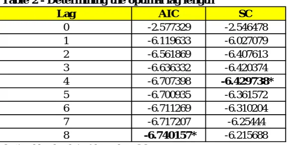
Table 2 shows that the optimal lag length given by SIC was 4.
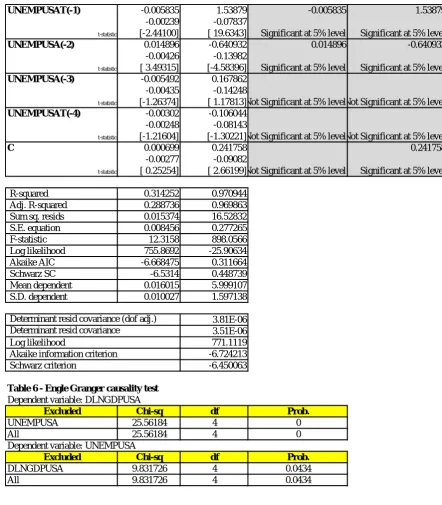
Table 3 shows that with the adjusted lag length, we arrived at the conclusions that at 4 lag lengths –
(i) The GDP has a negative effect on Unemployment with a magnitude of -6.203642 (lag 1) at
a significant level of 5%. The other lags were not significant at 5% level. Observed R square
of 97.0944% suggests that the movements in GDP can almost completely explain the
24
(ii) Unemployment is significant (at 5%) at 1 and 2 lags with magnitudes of -0.005835 and 0.014896 respectively whilst results at lags 3 and 4 are not significant at 5% level. However,
it is worth mentioning that the resulting R Square is only 31.4252%, which means that only
31% variations in GDP can only be explained by movements in Unemployment.
Table 4 shows that the Engle-Granger showed that unemployment and GDP causes each other at 5% level of significance.
France - refer to Appendix 2 and relevant tables
Table 1 shows that the ADF results Unit Root tests for GDP and Unemployment. lnGDP of France was shown to have a unit root (I(1)). Following this we took the first difference and
found that dlnGDP for France does not have a unit root (I (0)). The Unemployment also is
shown to have a unit root (I (1)). We again took the first difference and found that
dunemployment did not have a unit root (I (0)). Since these variables are integrated at the
same level, we did a test for co-integration.
Table 2 & 3 shows the results of the co-integration by verifying whether the residual (regressing lnGDPFRANCE against UNEMPFRANCE) is stationary and we found that no
co-integration existed. Since there is no co-integration, the VAR approach can be used.
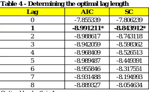
Table 4 shows the optimal lag length given by SIC is 1.
Table 5 shows that with the adjusted lag length we see that the results are not significant at 5% for both GDP and Unemployment, suggesting that change in GDP does not cause a
change in Unemployment and vice versa.
Table 6 shows that the Granger Causality test at 5% level of significance confirms the above finding that neither unemployment nor GDP has effect on the other variable.
Japan - refer to Appendix 3 and relevant tables
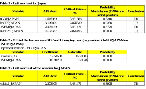
Table 1 shows the results of the ADF Unit Root tests for GDP and Unemployment for Japan. lnGDP of Japan was shown to have a unit root (I(1)). Following this we took the first
difference and found that dlnGDP does not have a unit root (I (0)). The Unemployment is,
however, shown to have a unit root (I (1)). We took the first difference and found that
dunemployment did not have a unit root (I (0)). Since these are integrated at the same level,
25
Table 2 & 3 shows that there was no co-integration. Since no co-integration existed, we proceeded with the VAR approach.
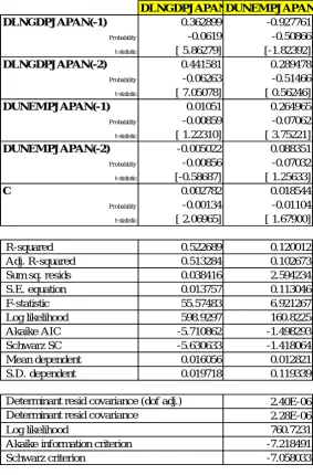
Table 4 shows the optimal lag length given by SIC is 2.
Table 5 shows that with the adjusted lag length we see that the results are not significant at 5% for both GDP and Unemployment, suggesting that change in GDP does not cause a
change in Unemployment and vice versa.
Table 6 shows that from the Granger Causality test at 5% level of significance, it can be seen that it confirms the above finding that neither unemployment nor GDP has effect on the other
variable.
6.
Main Conclusions
Okun’s law does not appear to hold in our samples. In the USA, there is two-way causality between the variables, but varying directions of effect. In Japan and France, there is no
causality between the variables.
In the USA, we discovered that GDP and Unemployment have causation effects on each
other at a significant level: a 1% change in GDP leads to approximately negative 6 % change in unemployment. This shows that the Okun’s Law of positive GDP change having a negative impact on unemployment holds for USA. As for the unemployment, we found that
unemployment had either a positive or a negative impact on GDP in two respective periods.
The Engle Granger causality shows that unemployment does cause change in GDP. The low
R Square indicates while change in unemployment does explain changes in GDP, while there
are other factors that explain the rest of the approximate 70% movement in GDP. With this
information we can conclude that there is causation from a change in unemployment on GDP,
but the direction of the change is undetermined.
In France and Japan, the results show that the variables have no effect on each other. This
shows that any correlation one might gather between the variables is not an indicator of
direction or magnitude of change in the other.
Arthur Okun originally observed the effect of unemployment and GDP in the USA. With
the data we have obtained up to the current day, it is shown that there is still an effect
between the two. GDP does have a negative effect on unemployment, as was hypothesized
by Okun, yet the magnitude (6) is larger than was hypothesized (3). Unemployment also
26
negatively, it affected GDP since it caused a negative change in time lag 1 but caused a
positive change in time lag 2.
With the other two countries, the lack of causality shows that GDP and unemployment have no effect on each other. As we wanted to check Okun’s law on countries in different geographical regions, we can see that it does not hold. Although, the geography cannot be a
determined reason, it could be from many other factors, it does show that Okun’s law does
not hold for every country.
Possible reasons of non-causality could be that Japan for instance has a large manufacturing
sector which can produce much without increase of employment level: the future scope for
employment could be reduced if existing businesses can produce more output using existing
labor more intensively and employing additional capital equipment to that end. A highly
protected labor market in France may suggest a low reaction of employment to GDP
movements and vice versa and hence gives ground to the above statistical results. However,
further analysis should be conducted to explain the nonexistence of causality of employment
on GDP for France and Japan and vice versa, as detailed in the next section.
7.
Further Discussion
To further enhance our current model and conclusions, we would examine Okun’s law with additional variables such as labor productivity, average working hours, and size of working
population (which are all key components of explaining output growth apart from
unemployment).
Also, we employed a long time series in this study but history can actually hide changes in
relationships: we can further improve the study by estimating over shorter time series while
taking into consideration the various important events in history such as economic crises,
significant changes in policies and regulation for example.
The Okun’s law was thought of in 1962 and we expect that the relationship between unemployment to output growth should not necessarily hold for all countries due to
differences in legal systems, social customs, demographics, usage of IT, tastes, states of
business cycle and cultures.
It is worth mentioning that unemployment rates can be largely affected by the labor regulation prevailing in one’s country: for instance, heavily regulated labor markets will tend to have higher unemployment whereas lower regulated labor markets will have lower
27
8.
References
Altig, D., Terry, F., & Rupert, P. (1997). Okun's Law Revisited: Should We Worry about
Low Unemployment? . Federal Reserve Bank of Cleveland. Economic Commentary., 1-4. Retrieved from http://proxy1.library.ln.edu.hk:2197/docview/233608458?
accountid=12107.
Burgen, E., Meyer, B., & Tasci, M. (2012). An Elusive Relation between Unemployment and GDP Growth: Okun’s Law. Federal Reserve Bank of Cleverland., Retrieved from http://www.clevelandfed.org/research/trends/2012/0412/01labmar.cfm
Chamberlin, G. (2011). Okun's Law Revisited. Economic & Labour Market Review, 5(2),
104-132. Retrieved from http://proxy1.library.ln.edu.hk:2197/docview/
857921570?accountid=12107.
Irfan, L., Muhammad S., Jalil, M. et al. (2012). Test of Okun’s Law in Some Asian
Countries:Co-integration Approach. Retrieved from
http://dx.doi.org/10.2139/ssrn.1562602
Kitov, I., & Kitov, O. (2012). Modeling Unemployment and Employment in Advanced
Economies: Okun's Law with a Structural Break. Theoretical and Practical Research
in Economic Fields,3(1), 26-41. Retrieved
from http://proxy1.library.ln.edu.hk:2197/docview/1038147682?accountid=12107.
Neely , C. (2010). Okun's Law: Output and Unemployment. Federal Reserve Bank of
St.Louis. , Retrieved from http://research.stlouisfed.org/publications/es/10/ES1004.pdf).
Okun, A. M. (1962). Potential GNP: Its Measurement and Significance. Proceedings of the
Business and Economic Statistics Section of the American Statistical Association.,
89-104.
Organisation For Economic Co-operation and Development. (2012). OECD Statextracts.
Retrieved from http://stats.oecd.org/Index.aspx?QueryId=350
Owyang, M., & Sekhposyan, T. (2012). Okun's Law over the Business Cycle: Was the
Recession Really that Different? Federal Reserve of St. Louis., Retrieved from
http://research.stlouisfed.org/publications/review/12/09/399-418Owyang_rev.pdf.
Wen, Y., & Chen, M. (2012). Okun’s Law: A Meaningful Guide for Monetary Policy?.
Federal Reserve Bank of St.Louis., Retrieved from http://research.stlouisfed.org/
28
9.
Appendix
Appendix 1 - Regression results for USA
Table 1 - Unit root te st for USA
Variable ADF-te st Critical Value
-5%
Probability MacKinnon (1996) one
side d p-value s
Conclusion
lnGDPUSA 0.808482 -3.429834 0.9998 I(I) dlnGDPUSA -6.613013 -2.874143 0.0000 I(0) UNEMPUSA -3.868535 -3.429745 0.0149 I(0) Since dlnGDPUSA is I(0) and UNEMPUSA is I(0), we use VAR approach
Table 2 - De te rmining the optimal lag le ngth
Lag AIC SC
0 -2.577329 -2.546478 1 -6.119633 -6.027079 2 -6.561869 -6.407613 3 -6.636332 -6.420374 4 -6.707398 -6.429738*
5 -6.700935 -6.361572 6 -6.711269 -6.310204 7 -6.717207 -6.25444
8 -6.740157* -6.215688
29
UNEMPUSAT(-1) -0.005835 1.53879 -0.005835 1.53879
-0.00239 -0.07837
t-statistic [-2.44100] [ 19.6343] Significant at 5% level Significant at 5% level
UNEMPUSA(-2) 0.014896 -0.640932 0.014896 -0.640932
-0.00426 -0.13982
t-statistic [ 3.49315] [-4.58396] Significant at 5% level Significant at 5% level UNEMPUSA(-3) -0.005492 0.167862
-0.00435 -0.14248
t-statistic [-1.26374] [ 1.17813]Not Significant at 5% levelNot Significant at 5% level UNEMPUSAT(-4) -0.00302 -0.106044
-0.00248 -0.08143
t-statistic [-1.21604] [-1.30221]Not Significant at 5% levelNot Significant at 5% level
C 0.000699 0.241758 0.241758
-0.00277 -0.09082
t-statistic [ 0.25254] [ 2.66199]Not Significant at 5% level Significant at 5% level
R-squared 0.314252 0.970944
Adj. R-squared 0.288736 0.969863 Sum sq. resids 0.015374 16.52832 S.E. equation 0.008456 0.277265
F-statistic 12.3158 898.0566
Log likelihood 755.8692 -25.90634
Akaike AIC -6.668475 0.311664
Schwarz SC -6.5314 0.448739
Mean dependent 0.016015 5.999107 S.D. dependent 0.010027 1.597138
3.81E-06 3.51E-06 771.1119 -6.724213 -6.450063
Table 6 - Engle Granger causality test Dependent variable: DLNGDPUSA
Excluded Chi-sq df Prob.
UNEMPUSA 25.56184 4 0
All 25.56184 4 0
Dependent variable: UNEMPUSA
Excluded Chi-sq df Prob.
DLNGDPUSA 9.831726 4 0.0434
All 9.831726 4 0.0434
Determinant resid covariance (dof adj.) Determinant resid covariance
Log likelihood
30
Table 4 - Engle Grange r causality te st
Dependent variable: DLNGDPUSA
Exclude d Chi-sq df Prob.
UNEMPUSA 25.56184 4 0
All 25.56184 4 0
Dependent variable: UNEMPUSA
Exclude d Chi-sq df Prob.
DLNGDPUSA 9.831726 4 0.0434
All 9.831726 4 0.0434
10.Appendix 2 - Regression results for France
Table 1 - Unit root te st for France
Variable ADF-te st Critical
Value - 5%
Probability MacKinnon (1996) one
side d p-value s
Conclusion
lnGDPFRANCe -2.434247 -3.448681 0.3602 I(I) dlnGDPUSA -4.742218 -2.886290 0.0001 I(0) UNEMPUSA -3.064003 -3.448681 0.1199 I(I) dUNEMPUSA -4.031055 -2.886290 0.0018 I(0)
Dependent variable - lnGDPFRANCE
Variable Coe fficie nt t-statistic Probability
Constant (C ) 13.50065 50.37220 0.0000 UNEMPFRANCE 0.059801 2.085581 0.0392
Table 3 - Unit root re st of the re sidual for France
Variable ADF-te st Critical
Value - 5%
Probability MacKinnon (1996) one
side d p-value s
Conclusion
residual_FRANCE -2.400196 -3.448681 0.3776 I(I)
Conclusion: Since probability > 0.05, we accept the hypothesis that residual_FRANCE has a unit root. Therefore, GDP and Unemployment for FRANCE are not co-integrated
Table 4 - De te rmining the optimal lag le ngth
Lag AIC SC
0 -7.855339 -7.806239
1 -8.991211* -8.843912*
2 -8.988617 -8.743118 3 -8.942059 -8.598362 4 -8.968409 -8.526513 5 -8.989487 -8.449391 6 -8.955846 -8.317551 7 -8.931488 -8.194993 8 -8.889327 -8.054634 Optimal lag lenth is 1
Table 2 - OLS of the two se rie s - GDP and Une mployme nt (re gre ssion of lnGDPFRANCE on UNEMPFRANCE)
31 Appendix 3 - Regression results for Japan
Table 1 - Unit root te st for Japan
Variable ADF-te st Critical Value -5%
Probability MacKinnon (1996) one
side d p-value s
Conclusion
lnGDPJAPAN -1.516989 -3.431368 0.8210 I(I)
dlnGDPJAPAN -3.100604 -2.875330 0.0280 I(0)
UNEMPJAPAN -2.401129 -3.431471 0.3779 I(I)
dUNEMPJAPAN -10.32337 -2.875195 0.0000 I(0)
Dependent variable - lnGDPJAPAN
Variable Coe fficie nt t-statistic Probability
Constant (C ) 17.54558 158.3603 0.0000
UNEMPJAPAN 0.594233 16.3344 0.0000
Table 3 - Unit root re st of the re sidual for JAPAN
Variable ADF-te st Critical Value -5%
Probability MacKinnon (1996) one
side d p-value s
Conclusion
residual_JAPAN -2.373105 -3.431471 0.3925 I(I)
Conclusion: Since probability > 0.05, we accept the hypothesis that residual_JAPAN has a unit root. Therefore, GDP and Unemployment for JAPAN are not co-integrated
Table 4 - De te rmining the optimal lag le ngth
Lag AIC SC
0 -6.488567 -6.455812
1 -7.031031 -6.932766
2 -7.232764 -7.068988*
3 -7.245318 -7.016033
4 -7.24958 -6.954784
5 -7.277654 -6.917348
6 -7.276253 -6.850436
7 -7.269277 -6.77795
8 -7.327456* -6.770619
Optimal lag lenth is 2
Table 2 - OLS of the two se rie s - GDP and Une mployme nt (re gre ssion of lnGDPJAPAN on UNEMPJAPAN)
32
Table 5 - Ve ctor Autogre ssion Estimate s base d on lag le ngth of 2
DLNGDPJAPANDUNEMPJAPAN DLNGDPJAPAN(-1) 0.362899 -0.927761
Probability -0.0619 -0.50866 t-statistic [ 5.86279] [-1.82392]
DLNGDPJAPAN(-2) 0.441581 0.289478
Probability -0.06263 -0.51466 t-statistic [ 7.05078] [ 0.56246]
DUNEMPJAPAN(-1) 0.01051 0.264965
Probability -0.00859 -0.07062 t-statistic [ 1.22310] [ 3.75221] DUNEMPJAPAN(-2) -0.005022 0.088351 Probability -0.00856 -0.07032 t-statistic [-0.58687] [ 1.25633]
C 0.002782 0.018544
Probability -0.00134 -0.01104 t-statistic [ 2.06965] [ 1.67900]
R-squared 0.522689 0.120012
Adj. R-squared 0.513284 0.102673
Sum sq. resids 0.038416 2.594234
S.E. equation 0.013757 0.113046
F-statistic 55.57483 6.921267
Log likelihood 598.9297 160.8225
Akaike AIC -5.710862 -1.498293
Schwarz SC -5.630633 -1.418064
Mean dependent 0.016056 0.012821
S.D. dependent 0.019718 0.119339
2.40E-06 2.28E-06 760.7231 -7.218491 -7.058033
Table 6 - Engle Grange r causality te st Dependent variable: DLNGDPJAPAN
Exclude d Chi-sq df Prob.
DUNEMPJAPAN 1.558921 2 0.4587
All 1.558921 2 0.4587
Dependent variable: DUNEMPJAPAN
Exclude d Chi-sq df Prob.
DLNGDPJAPAN 3.797792 2 0.1497
All 3.797792 2 0.1497
Schwarz criterion
Determinant resid covariance (dof adj.) Determinant resid covariance
Log likelihood
33
Appendix 4 - Raw data from OECD for USA from 1955 Q1 to 2012 Q3
Quarter GDP [Millions of National Currency] Unemployment rate [% ] Quarter GDP [Millions of National Currency] Unemployment rate [% ] Quarter GDP [Millions of National Currency] Unemployment rate [% ]
Q1-1955 402,600 4.733333333 Q2-1974 1,484,800 5.200000000 Q3-1993 6,688,300 6.800000000 Q2-1955 410,900 4.400000000 Q3-1974 1,513,700 5.633333333 Q4-1993 6,813,800 6.633333333 Q3-1955 419,400 4.100000000 Q4-1974 1,552,800 6.600000000 Q1-1994 6,916,300 6.566666667 Q4-1955 426,000 4.233333333 Q1-1975 1,569,400 8.266666667 Q2-1994 7,044,300 6.200000000 Q1-1956 428,300 4.033333333 Q2-1975 1,605,000 8.866666667 Q3-1994 7,131,800 6.000000000 Q2-1956 434,200 4.200000000 Q3-1975 1,662,400 8.466666667 Q4-1994 7,248,200 5.633333333 Q3-1956 439,200 4.133333333 Q4-1975 1,713,900 8.300000000 Q1-1995 7,307,700 5.466666667 Q4-1956 448,100 4.133333333 Q1-1976 1,771,900 7.733333333 Q2-1995 7,355,800 5.666666667 Q1-1957 457,200 3.933333333 Q2-1976 1,804,200 7.566666667 Q3-1995 7,452,500 5.666666667 Q2-1957 459,200 4.100000000 Q3-1976 1,837,700 7.733333333 Q4-1995 7,542,500 5.566666667 Q3-1957 466,400 4.233333333 Q4-1976 1,884,500 7.766666667 Q1-1996 7,638,200 5.533333333 Q4-1957 461,500 4.933333333 Q1-1977 1,938,500 7.500000000 Q2-1996 7,800,000 5.500000000 Q1-1958 453,900 6.300000000 Q2-1977 2,005,200 7.133333333 Q3-1996 7,892,700 5.266666667 Q2-1958 458,000 7.366666667 Q3-1977 2,066,000 6.900000000 Q4-1996 8,023,000 5.333333333 Q3-1958 471,700 7.333333333 Q4-1977 2,110,800 6.666666667 Q1-1997 8,137,000 5.233333333 Q4-1958 485,000 6.366666667 Q1-1978 2,149,100 6.333333333 Q2-1997 8,276,800 5.000000000 Q1-1959 495,500 5.833333333 Q2-1978 2,274,700 6.000000000 Q3-1997 8,409,900 4.866666667 Q2-1959 508,500 5.100000000 Q3-1978 2,335,200 6.033333333 Q4-1997 8,505,700 4.666666667 Q3-1959 509,300 5.266666667 Q4-1978 2,416,000 5.900000000 Q1-1998 8,600,600 4.633333333 Q4-1959 513,200 5.600000000 Q1-1979 2,463,300 5.866666667 Q2-1998 8,698,600 4.400000000 Q1-1960 527,000 5.133333333 Q2-1979 2,526,400 5.700000000 Q3-1998 8,847,200 4.533333333 Q2-1960 526,200 5.233333333 Q3-1979 2,599,700 5.866666667 Q4-1998 9,027,500 4.433333333 Q3-1960 529,000 5.533333333 Q4-1979 2,659,400 5.966666667 Q1-1999 9,148,600 4.300000000 Q4-1960 523,700 6.266666667 Q1-1980 2,724,100 6.300000000 Q2-1999 9,252,600 4.266666667 Q1-1961 528,000 6.800000000 Q2-1980 2,728,000 7.333333333 Q3-1999 9,405,100 4.233333333 Q2-1961 539,000 7.000000000 Q3-1980 2,785,200 7.666666667 Q4-1999 9,607,700 4.066666667 Q3-1961 549,500 6.766666667 Q4-1980 2,915,300 7.400000000 Q1-2000 9,709,500 4.033333333 Q4-1961 562,600 6.200000000 Q1-1981 3,051,400 7.433333333 Q2-2000 9,949,100 3.933333333 Q1-1962 576,100 5.633333333 Q2-1981 3,084,300 7.400000000 Q3-2000 10,017,500 4.000000000 Q2-1962 583,200 5.533333333 Q3-1981 3,177,000 7.400000000 Q4-2000 10,129,800 3.900000000 Q3-1962 590,000 5.566666667 Q4-1981 3,194,700 8.233333333 Q1-2001 10,165,100 4.233333333 Q4-1962 593,300 5.533333333 Q1-1982 3,184,900 8.833333333 Q2-2001 10,301,300 4.400000000 Q1-1963 602,500 5.766666667 Q2-1982 3,240,900 9.433333333 Q3-2001 10,305,200 4.833333333 Q2-1963 611,200 5.733333333 Q3-1982 3,274,400 9.900000000 Q4-2001 10,373,100 5.500000000 Q3-1963 623,900 5.500000000 Q4-1982 3,312,500 10.666666670 Q1-2002 10,498,700 5.700000000 Q4-1963 633,500 5.566666667 Q1-1983 3,381,000 10.366666670 Q2-2002 10,601,900 5.833333333 Q1-1964 649,600 5.466666667 Q2-1983 3,482,200 10.133333330 Q3-2002 10,701,700 5.733333333 Q2-1964 658,900 5.200000000 Q3-1983 3,587,100 9.366666667 Q4-2002 10,766,900 5.866666667 Q3-1964 670,500 5.000000000 Q4-1983 3,688,100 8.533333333 Q1-2003 10,887,400 5.866666667 Q4-1964 675,600 4.966666667 Q1-1984 3,807,400 7.866666667 Q2-2003 11,011,600 6.133333333 Q1-1965 695,700 4.900000000 Q2-1984 3,906,300 7.433333333 Q3-2003 11,255,100 6.133333333 Q2-1965 708,100 4.666666667 Q3-1984 3,976,000 7.433333333 Q4-2003 11,414,800 5.833333333 Q3-1965 725,200 4.366666667 Q4-1984 4,034,000 7.300000000 Q1-2004 11,589,900 5.700000000 Q4-1965 747,500 4.100000000 Q1-1985 4,117,200 7.233333333 Q2-2004 11,762,900 5.600000000 Q1-1966 770,800 3.866666667 Q2-1985 4,175,700 7.300000000 Q3-2004 11,936,300 5.433333333 Q2-1966 779,900 3.833333333 Q3-1985 4,258,300 7.200000000 Q4-2004 12,123,900 5.433333333 Q3-1966 793,100 3.766666667 Q4-1985 4,318,700 7.033333333 Q1-2005 12,361,800 5.300000000 Q4-1966 806,900 3.700000000 Q1-1986 4,382,400 7.033333333 Q2-2005 12,500,000 5.100000000 Q1-1967 817,800 3.833333333 Q2-1986 4,423,200 7.166666667 Q3-2005 12,728,600 4.966666667 Q2-1967 822,300 3.833333333 Q3-1986 4,491,300 6.966666667 Q4-2005 12,901,400 4.966666667 Q3-1967 837,000 3.800000000 Q4-1986 4,543,300 6.833333333 Q1-2006 13,161,400 4.733333333 Q4-1967 852,700 3.900000000 Q1-1987 4,611,100 6.600000000 Q2-2006 13,330,400 4.633333333 Q1-1968 879,800 3.733333333 Q2-1987 4,686,700 6.266666667 Q3-2006 13,432,800 4.633333333 Q2-1968 904,100 3.566666667 Q3-1987 4,764,500 6.000000000 Q4-2006 13,584,200 4.433333333 Q3-1968 919,300 3.533333333 Q4-1987 4,883,100 5.833333333 Q1-2007 13,758,500 4.500000000 Q4-1968 936,200 3.400000000 Q1-1988 4,948,600 5.700000000 Q2-2007 13,976,800 4.500000000 Q1-1969 960,900 3.400000000 Q2-1988 5,059,300 5.466666667 Q3-2007 14,126,200 4.666666667 Q2-1969 976,100 3.433333333 Q3-1988 5,142,800 5.466666667 Q4-2007 14,253,200 4.800000000 Q3-1969 996,300 3.566666667 Q4-1988 5,251,000 5.333333333 Q1-2008 14,273,900 5.000000000 Q4-1969 1,004,500 3.566666667 Q1-1989 5,360,300 5.200000000 Q2-2008 14,415,500 5.333333333 Q1-1970 1,017,100 4.166666667 Q2-1989 5,453,600 5.233333333 Q3-2008 14,395,100 6.000000000 Q2-1970 1,033,100 4.766666667 Q3-1989 5,532,900 5.233333333 Q4-2008 14,081,700 6.866666667 Q3-1970 1,050,500 5.166666667 Q4-1989 5,581,700 5.366666667 Q1-2009 13,923,400 8.266666667 Q4-1970 1,052,700 5.833333333 Q1-1990 5,708,100 5.300000000 Q2-2009 13,885,400 9.266666667 Q1-1971 1,098,100 5.933333333 Q2-1990 5,797,400 5.333333333 Q3-2009 13,952,200 9.633333333 Q2-1971 1,118,800 5.900000000 Q3-1990 5,850,600 5.700000000 Q4-2009 14,133,600 9.933333333 Q3-1971 1,139,100 6.033333333 Q4-1990 5,846,000 6.133333333 Q1-2010 14,270,300 9.766666667 Q4-1971 1,151,400 5.933333333 Q1-1991 5,880,200 6.600000000 Q2-2010 14,413,500 9.633333333 Q1-1972 1,190,100 5.766666667 Q2-1991 5,962,000 6.833333333 Q3-2010 14,576,000 9.533333333 Q2-1972 1,225,600 5.700000000 Q3-1991 6,033,700 6.866666667 Q4-2010 14,735,900 9.566666667 Q3-1972 1,249,300 5.566666667 Q4-1991 6,092,500 7.100000000 Q1-2011 14,814,900 9.000000000 Q4-1972 1,286,600 5.366666667 Q1-1992 6,190,700 7.366666667 Q2-2011 15,003,600 9.033333333 Q1-1973 1,335,100 4.933333333 Q2-1992 6,295,200 7.600000000 Q3-2011 15,163,200 9.066666667 Q2-1973 1,371,500 4.933333333 Q3-1992 6,389,700 7.633333333 Q4-2011 15,321,000 8.700000000 Q3-1973 1,390,700 4.800000000 Q4-1992 6,493,600 7.366666667 Q1-2012 15,478,300 8.266666667 Q4-1973 1,431,800 4.766666667 Q1-1993 6,544,500 7.133333333 Q2-2012 15,585,600 8.166666667 Q1-1974 1,446,500 5.133333333 Q2-1993 6,622,700 7.066666667 Q3-2012 15,775,700 8.066666667
USA
34 Quarter GDP [Millions of National Currency] Unemployment rate [% ] Quarter GDP [Millions of National Currency] Unemployment rate [% ]
Q1-1983 614,196 6.900000000 Q1-1998 1,303,952 10.866666670 Q2-1983 631,032 6.933333333 Q2-1998 1,320,132 10.733333330 Q3-1983 647,984 7.200000000 Q3-1998 1,326,548 10.700000000 Q4-1983 661,980 7.566666667 Q4-1998 1,335,568 10.700000000 Q1-1984 679,060 8.100000000 Q1-1999 1,343,868 10.766666670 Q2-1984 689,724 8.500000000 Q2-1999 1,356,884 10.600000000 Q3-1984 702,960 8.666666667 Q3-1999 1,372,404 10.266666670 Q4-1984 709,420 8.833333333 Q4-1999 1,391,336 9.866666667 Q1-1985 722,980 8.900000000 Q1-2000 1,416,816 9.500000000 Q2-1985 740,144 8.933333333 Q2-2000 1,432,060 9.100000000 Q3-1985 752,164 9.000000000 Q3-2000 1,447,636 8.866666667 Q4-1985 765,304 9.000000000 Q4-2000 1,466,768 8.566666667 Q1-1986 780,652 8.933333333 Q1-2001 1,480,932 8.266666667 Q2-1986 796,904 9.066666667 Q2-2001 1,493,052 8.133333333 Q3-1986 810,208 9.133333333 Q3-2001 1,504,252 8.100000000 Q4-1986 816,036 9.233333333 Q4-2001 1,507,416 8.200000000 Q1-1987 820,104 9.366666667 Q1-2002 1,525,736 8.000000000 Q2-1987 833,896 9.366666667 Q2-2002 1,538,648 8.200000000 Q3-1987 845,784 9.200000000 Q3-2002 1,551,312 8.433333333 Q4-1987 864,880 9.133333333 Q4-2002 1,559,684 8.600000000 Q1-1988 883,344 9.033333333 Q1-2003 1,569,620 8.633333333 Q2-1988 897,100 8.833333333 Q2-2003 1,577,460 8.866666667 Q3-1988 915,932 8.800000000 Q3-2003 1,595,408 8.866666667 Q4-1988 935,440 8.666666667 Q4-2003 1,613,432 9.166666667 Q1-1989 955,804 8.533333333 Q1-2004 1,628,452 9.300000000 Q2-1989 971,348 8.400000000 Q2-2004 1,644,772 9.200000000 Q3-1989 986,692 8.300000000 Q3-2004 1,658,336 9.266666667 Q4-1989 1,005,220 8.200000000 Q4-2004 1,681,188 9.266666667 Q1-1990 1,020,852 8.100000000 Q1-2005 1,692,180 9.100000000 Q2-1990 1,031,020 8.000000000 Q2-2005 1,705,628 9.200000000 Q3-1990 1,037,788 7.933333333 Q3-2005 1,720,436 9.366666667 Q4-1990 1,043,012 8.000000000 Q4-2005 1,746,132 9.500000000 Q1-1991 1,051,216 8.033333333 Q1-2006 1,765,360 9.500000000 Q2-1991 1,068,716 8.300000000 Q2-2006 1,790,944 9.366666667 Q3-1991 1,078,672 8.600000000 Q3-2006 1,804,796 9.233333333 Q4-1991 1,089,204 8.800000000 Q4-2006 1,836,260 8.900000000 Q1-1992 1,104,888 9.000000000 Q1-2007 1,857,804 8.766666667 Q2-1992 1,105,700 9.200000000 Q2-2007 1,877,656 8.500000000 Q3-1992 1,109,728 9.433333333 Q3-2007 1,898,196 8.300000000 Q4-1992 1,108,856 9.700000000 Q4-2007 1,915,864 7.900000000 Q1-1993 1,111,280 10.000000000 Q1-2008 1,938,784 7.533333333 Q2-1993 1,116,332 10.400000000 Q2-2008 1,934,472 7.700000000 Q3-1993 1,122,240 10.800000000 Q3-2008 1,933,504 7.833333333 Q4-1993 1,128,544 11.066666670 Q4-2008 1,920,172 8.200000000 Q1-1994 1,136,248 11.233333330 Q1-2009 1,887,172 8.900000000 Q2-1994 1,152,512 11.266666670 Q2-2009 1,879,696 9.466666667 Q3-1994 1,161,668 11.100000000 Q3-2009 1,881,480 9.600000000 Q4-1994 1,176,532 10.800000000 Q4-2009 1,896,096 9.966666667 Q1-1995 1,184,764 10.566666670 Q1-2010 1,910,924 9.900000000 Q2-1995 1,193,992 10.533333330 Q2-2010 1,928,572 9.700000000 Q3-1995 1,200,888 10.366666670 Q3-2010 1,946,632 9.666666667 Q4-1995 1,206,672 10.633333330 Q4-2010 1,957,828 9.666666667 Q1-1996 1,219,044 10.900000000 Q1-2011 1,981,276 9.600000000 Q2-1996 1,223,780 10.900000000 Q2-2011 1,989,364 9.600000000 Q3-1996 1,231,112 10.966666670 Q3-2011 2,000,492 9.600000000 Q4-1996 1,233,272 11.033333330 Q4-2011 2,010,592 9.766666667 Q1-1997 1,242,672 11.233333330 Q1-2012 2,016,132 10.000000000 Q2-1997 1,258,068 11.200000000 Q2-2012 2,025,908 10.266666670 Q3-1997 1,270,488 11.133333330 Q3-2012 2,038,568 10.700000000 Q4-1997 1,288,124 11.000000000
35
Appendix 6 - Raw data from OECD for JAPAN from 1960 Q 1 to 2012 Q3
Quarter
GDP [Millions of
National Currency] Unemployment rate [% ] Quarter GDP [Millions of
National Currency] Unemployment rate [% ] Quarter GDP [Millions of
National Currency]
Unemployment rate [% ]
Q1-1960 15,549,191 1.766666667 Q4-1977 196,902,817 2.000000000 Q3-1995 504,785,500 3.166666667
Q2-1960 15,756,762 1.666666667 Q1-1978 202,890,186 2.166666667 Q4-1995 505,200,400 3.333333333
Q3-1960 16,654,119 1.566666667 Q2-1978 206,791,482 2.266666667 Q1-1996 506,644,300 3.366666667
Q4-1960 17,460,817 1.466666667 Q3-1978 212,164,751 2.300000000 Q2-1996 511,811,800 3.400000000
Q1-1961 18,417,553 1.433333333 Q4-1978 216,170,757 2.200000000 Q3-1996 511,793,300 3.333333333
Q2-1961 19,172,871 1.466666667 Q1-1979 220,537,038 2.100000000 Q4-1996 518,248,600 3.366666667
Q3-1961 19,920,292 1.433333333 Q2-1979 225,494,138 2.033333333 Q1-1997 522,125,700 3.333333333
Q4-1961 21,434,312 1.433333333 Q3-1979 228,917,939 2.133333333 Q2-1997 523,481,000 3.333333333
Q1-1962 21,975,188 1.300000000 Q4-1979 232,316,510 2.066666667 Q3-1997 523,981,400 3.433333333
Q2-1962 22,325,413 1.300000000 Q1-1980 236,367,024 1.900000000 Q4-1997 524,552,900 3.500000000
Q3-1962 22,466,631 1.233333333 Q2-1980 241,174,504 1.966666667 Q1-1998 514,034,200 3.666666667
Q4-1962 22,984,432 1.333333333 Q3-1980 248,997,868 2.033333333 Q2-1998 510,589,500 4.066666667
Q1-1963 23,741,903 1.400000000 Q4-1980 257,143,481 2.166666667 Q3-1998 510,483,200 4.266666667
Q2-1963 25,113,885 1.200000000 Q1-1981 259,587,692 2.200000000 Q4-1998 513,700,300 4.400000000
Q3-1963 26,224,351 1.200000000 Q2-1981 264,089,963 2.266666667 Q1-1999 506,806,200 4.600000000
Q4-1963 27,553,874 1.233333333 Q3-1981 264,936,719 2.166666667 Q2-1999 506,745,700 4.733333333
Q1-1964 28,646,393 1.233333333 Q4-1981 269,482,098 2.200000000 Q3-1999 503,511,900 4.700000000
Q2-1964 29,984,327 1.166666667 Q1-1982 275,023,237 2.233333333 Q4-1999 504,332,000 4.633333333
Q3-1964 30,668,676 1.166666667 Q2-1982 276,506,987 2.333333333 Q1-2000 511,596,600 4.833333333
Q4-1964 31,505,526 1.100000000 Q3-1982 278,338,143 2.366666667 Q2-2000 510,311,500 4.700000000
Q1-1965 32,509,232 1.133333333 Q4-1982 281,797,994 2.466666667 Q3-2000 508,162,200 4.666666667
Q2-1965 33,265,780 1.233333333 Q1-1983 283,880,194 2.666666667 Q4-2000 510,617,500 4.733333333
Q3-1965 34,330,404 1.266666667 Q2-1983 286,953,285 2.666666667 Q1-2001 514,323,900 4.766666667
Q4-1965 34,415,422 1.300000000 Q3-1983 290,858,526 2.700000000 Q2-2001 508,702,000 4.900000000
Q1-1966 36,458,832 1.366666667 Q4-1983 294,324,971 2.600000000 Q3-2001 501,054,200 5.133333333
Q2-1966 38,668,995 1.333333333 Q1-1984 299,474,582 2.700000000 Q4-2001 498,973,300 5.366666667
Q3-1966 40,143,942 1.300000000 Q2-1984 305,988,963 2.733333333 Q1-2002 499,072,600 5.266666667
Q4-1966 41,055,759 1.266666667 Q3-1984 310,779,402 2.733333333 Q2-2002 498,463,500 5.400000000
Q1-1967 43,149,420 1.300000000 Q4-1984 313,433,680 2.666666667 Q3-2002 499,677,500 5.433333333
Q2-1967 44,401,105 1.266666667 Q1-1985 321,223,672 2.566666667 Q4-2002 500,050,000 5.333333333
Q3-1967 46,709,926 1.166666667 Q2-1985 327,803,781 2.566666667 Q1-2003 494,130,900 5.333333333
Q4-1967 48,754,361 1.266666667 Q3-1985 332,263,450 2.600000000 Q2-2003 500,479,900 5.433333333
Q1-1968 50,567,124 1.266666667 Q4-1985 338,218,027 2.766666667 Q3-2003 500,306,600 5.166666667
Q2-1968 52,602,944 1.166666667 Q1-1986 341,426,530 2.666666667 Q4-2003 501,513,000 5.033333333
Q3-1968 54,592,820 1.200000000 Q2-1986 344,097,138 2.766666667 Q1-2004 505,660,900 4.900000000
Q4-1968 58,987,099 1.066666667 Q3-1986 346,821,708 2.833333333 Q2-2004 503,546,700 4.733333333
Q1-1969 59,103,909 1.133333333 Q4-1986 349,140,651 2.800000000 Q3-2004 503,540,700 4.766666667
Q2-1969 62,153,383 1.200000000 Q1-1987 348,081,901 2.933333333 Q4-2004 502,618,100 4.533333333
Q3-1969 64,693,569 1.133333333 Q2-1987 354,193,089 3.000000000 Q1-2005 501,045,500 4.533333333
Q4-1969 68,502,771 1.066666667 Q3-1987 362,183,004 2.766666667 Q2-2005 505,294,400 4.433333333
Q1-1970 71,303,755 1.066666667 Q4-1987 371,067,044 2.700000000 Q3-2005 504,882,100 4.300000000
Q2-1970 73,570,529 1.133333333 Q1-1988 380,745,703 2.666666667 Q4-2005 504,852,900 4.433333333
Q3-1970 76,687,484 1.233333333 Q2-1988 379,748,828 2.466666667 Q1-2006 505,439,500 4.200000000
Q4-1970 78,479,736 1.266666667 Q3-1988 389,351,109 2.533333333 Q2-2006 505,625,700 4.133333333
Q1-1971 79,831,104 1.166666667 Q4-1988 394,927,546 2.400000000 Q3-2006 504,301,100 4.100000000
Q2-1971 81,587,462 1.200000000 Q1-1989 408,101,863 2.333333333 Q4-2006 511,534,300 4.033333333
Q3-1971 83,785,217 1.233333333 Q2-1989 406,598,638 2.300000000 Q1-2007 514,027,200 4.000000000
Q4-1971 85,183,965 1.333333333 Q3-1989 416,229,726 2.200000000 Q2-2007 514,580,200 3.733333333
Q1-1972 89,342,674 1.400000000 Q4-1989 431,545,987 2.166666667 Q3-2007 510,185,400 3.733333333
Q2-1972 92,023,361 1.400000000 Q1-1990 431,437,353 2.133333333 Q4-2007 512,965,100 3.866666667
Q3-1972 96,184,634 1.433333333 Q2-1990 447,491,127 2.133333333 Q1-2008 513,557,200 3.933333333
Q4-1972 100,254,326 1.400000000 Q3-1990 456,061,031 2.066666667 Q2-2008 505,546,000 3.933333333
Q1-1973 107,239,556 1.233333333 Q4-1990 460,357,293 2.066666667 Q3-2008 496,533,900 3.966666667
Q2-1973 112,112,151 1.366666667 Q1-1991 467,578,555 2.100000000 Q4-2008 488,664,000 4.066666667
Q3-1973 116,418,848 1.266666667 Q2-1991 475,826,513 2.100000000 Q1-2009 468,119,700 4.600000000
Q4-1973 123,497,094 1.133333333 Q3-1991 476,606,729 2.100000000 Q2-2009 472,303,900 5.100000000
Q1-1974 126,432,527 1.300000000 Q4-1991 483,799,793 2.066666667 Q3-2009 469,530,700 5.400000000
Q2-1974 135,101,916 1.300000000 Q1-1992 484,967,886 2.066666667 Q4-2009 474,361,900 5.200000000
Q3-1974 141,413,153 1.400000000 Q2-1992 489,635,795 2.100000000 Q1-2010 479,058,700 5.066666667
Q4-1974 145,230,867 1.600000000 Q3-1992 489,658,719 2.166666667 Q2-2010 482,632,100 5.100000000
Q1-1975 145,512,278 1.766666667 Q4-1992 487,323,852 2.266666667 Q3-2010 484,851,300 5.033333333
Q2-1975 150,186,122 1.800000000 Q1-1993 494,406,557 2.300000000 Q4-2010 480,998,800 5.000000000
Q3-1975 153,577,412 1.900000000 Q2-1993 489,134,315 2.433333333 Q1-2011 469,423,800 4.766666667
Q4-1975 158,024,609 2.100000000 Q3-1993 487,864,181 2.533333333 Q2-2011 462,649,000 4.666666667
Q1-1976 163,372,752 2.033333333 Q4-1993 491,298,573 2.733333333 Q3-2011 472,142,100 4.433333333
Q2-1976 168,750,739 2.066666667 Q1-1994 495,078,200 2.866666667 Q4-2011 469,247,300 4.466666667
Q3-1976 173,854,801 2.000000000 Q2-1994 492,416,200 2.800000000 Q1-2012 475,642,900 4.533333333
Q4-1976 176,416,934 1.933333333 Q3-1994 500,154,300 2.966666667 Q2-2012 474,102,900 4.433333333
Q1-1977 183,985,701 1.966666667 Q4-1994 495,322,700 2.933333333 Q3-2012 469,793,500 4.233333333
Q2-1977 187,889,254 2.033333333 Q1-1995 495,185,500 3.033333333
Q3-1977 191,943,358 2.033333333 Q2-1995 501,233,400 3.066666667
36
11.
Abbreviations
lnGDPUSA Natural Logarithm form of GDP absolute values in U.S.A.
denominated in millions of U.S. dollars
dlnGDPUSA The First Difference of lnGDPUSA
UNEMPUSA Harmonised unemployment rates in U.S.A.
dUNEMPUSA The First Difference of the Harmonised unemployment rates in
U.S.A
lnGDPFRANCE Natural Logarithm form of GDP absolute values in France
denominated in millions of U.S. dollars
dlnGDPFRANCE The First Difference of lnGDPFRANCE
UNEMPFRANCE Harmonised unemployment rates in France
dUNEMPFRANCE The First Difference of the Harmonised unemployment rates in
France
lnGDPJAPAN Natural Logarithm form of GDP absolute values in Japan
denominated in millions of U.S. dollars
dlnGDPJAPAN The First Difference of lnGDPJAPAN
UNEMPJAPAN Harmonised unemployment rates in Japan
dUNEMPJAPAN The First Difference of the Harmonised unemployment rates in
Japan
VAR Vector Auto-regression
ECM Error Correction Model
AIC Akaike Information Criterion
SIC Schwarz Information Criteria
HP The HP trend of a variable captures not only the variable’s constant
37
12.
Graphs
USA
lnGDPUSA UNEMPUSA
dlnGDPUSA UNEMPUSA and dLNGDPUSA scatter diagram
USA
5.5 6.0 6.5 7.0 7.5 8.0 8.5 9.0 9.5 10.0
55 60 65 70 75 80 85 90 95 00 05 10
LNGDPUSA
3 4 5 6 7 8 9 10 11
55 60 65 70 75 80 85 90 95 00 05 10
UNEMPUSA
-.03 -.02 -.01 .00 .01 .02 .03 .04 .05 .06
55 60 65 70 75 80 85 90 95 00 05 10
DLNGDP
3 4 5 6 7 8 9 10 11
-.03 -.02 -.01 .00 .01 .02 .03 .04 .05 .06
DLNGDP
U
N
E
M
P
U
S
38
FRANCE
lnGDPFRANCE UNEMPFRANCE
dlnGDPFRANCE dUNEMPFRANCE
FRANCE
UNEMPUSA and dLNGDPUSA scatter diagram 13.2
13.4 13.6 13.8 14.0 14.2 14.4 14.6
10 20 30 40 50 60 70 80 90 100 110
LNGDP
6 7 8 9 10 11 12
10 20 30 40 50 60 70 80 90 100 110
UNEMP
-.02 -.01 .00 .01 .02 .03
10 20 30 40 50 60 70 80 90 100 110
DLNGDP
-.6 -.4 -.2 .0 .2 .4 .6 .8
10 20 30 40 50 60 70 80 90 100 110
DUNEMP
-.02 -.01 .00 .01 .02 .03
-.6 -.4 -.2 .0 .2 .4 .6 .8
DUNEMP
D
L
N
G
D
39
JAPAN
lnGDPJAPAN UNEMPJAPAN
dlnGDPJAPAN dUNEMPJAPAN
JAPAN
UNEMPJAPAN and dLNGDPJAPAN scatter diagram 16.5
17.0 17.5 18.0 18.5 19.0 19.5 20.0 20.5
25 50 75 100 125 150 175 200
LNGDP
1 2 3 4 5 6
25 50 75 100 125 150 175 200
UNEMP
-.06 -.04 -.02 .00 .02 .04 .06 .08
25 50 75 100 125 150 175 200
DLNGDP
-.3 -.2 -.1 .0 .1 .2 .3 .4 .5 .6
25 50 75 100 125 150 175 200
DUNEMP
-.06 -.04 -.02 .00 .02 .04 .06 .08
-.3 -.2 -.1 .0 .1 .2 .3 .4 .5 .6
DUNEMP
D
L
N
G
D