index forecast based on IMF data only

www.ann-geophys.net/24/989/2006/ © European Geosciences Union 2006

Annales

Geophysicae

Geomagnetic

D

st

index forecast based on IMF data only

G. Pallocchia, E. Amata, G. Consolini, M. F. Marcucci, and I. Bertello

Istituto di Fisica dello Spazio Interplanetario, Istituto Nazionale di Astrofisica, Rome, Italy

Received: 21 July 2005 – Revised: 8 February 2006 – Accepted: 14 February 2006 – Published: 19 May 2006

Abstract. In the past years several operationalDst

forecast-ing algorithms, based on both IMF and solar wind plasma parameters, have been developed and used. We describe an Artificial Neural Network (ANN) algorithm which calculates theDst index on the basis of IMF data only and discuss its

performance for several individual storms. Moreover, we briefly comment on the physical grounds which allow theDst

forecasting based on IMF only.

Keywords. Interplanetary physics (Interplanetary mag-netic fields) – Magnetospheric physics (Solar wind-magnetosphere interactions)

1 Introduction

It has been known for decades that solar activity influences the near-Earth environment through the solar wind variable flow and energetic particles emissions. The description of such influences and the development of tools for their now-casting and forenow-casting is the subject of space weather. It is now widely accepted that space weather effects may dam-age critical equipment, such as communication satellites or power lines and pipelines on the ground, and disrupt HF communications and GPS links, etc. As such, the prediction of space weather effects has both scientific and economical reasons.

In the framework of space weather an important role is played by geomagnetic storms, which are comprised of pro-cesses occurring in near-Earth space. During geomagnetic storms very intense fluctuations of the horizontal component of the ground magnetic field are observed (Gonzalez et al., 1994), due to variations in the equatorial ring current. A measure of these variations is provided by the Disturbance Storm Time index (Dst), which is calculated on an hourly

Correspondence to: G. Pallocchia

([email protected])

basis from measurements made by a network of four ground magnetometer stations at low and middle latitudes.

After the pioneering paper by Gosling (1993), CMEs are now widely recognized as the dominant interplanetary phe-nomenon responsible for intense magnetic storms. In the past years, many studies have been devoted to the relation betweenDst and solar wind conditions. Among them we

recall Gonzalez et al. (1999), who studied extensively the storm time profile and intensity in relation with the solar wind structures associated with CMEs and Corotating Inter-action Regions (CIRs), Kane (2005), who critically investi-gated the relationship of solar and interplanetary plasma pa-rameters with geomagnetic storms, and Gonzalez and Echer (2005), who studied the relationship between peakDst and

peak negativeBzduring intense geomagnetic storms;

more-over, we recall the recent review by Yermolaev et al. (2005) and all references therein. A complementary approach to these themes has been taken by several authors who tried to forecast Dst from measurements of Interplanetary

Mag-netic Field (IMF) and solar wind plasma parameters. As a result, a number of empirical models has been developed, based on differential equations (see, e.g. Burton et al., 1975; Fenrich and Luhmann, 1998; O’Brien and McPherron, 2000; Temerin and Li, 2002; Wang et al., 2003), and on Artificial Neural Networks (see, e.g. Wu and Lundstedt, 1997; Lund-stedt et al., 2002). All of them share the characteristics of having, as their inputs, both magnetic and plasma parame-ters of the solar wind, so that when, for some reason, some of the inputs are missing, the model predictions cannot be relied upon. This is more likely to occur with regard to the plasma parameters, as they are provided by instruments which can be affected by enhanced solar X-ray and energetic particle fluxes to a greater extent than magnetometers; moreover, at times the solar wind speed can exceed the upper instrumental limit.

Algorithm), based on an Artificial Neural Network (ANN), which computesDst from IMF data only. The aim of this

work was not to obtain the best possible algorithm for the

Dstprediction, but to build an operational service which can

reliably forecastDst on the basis of IMF data only.

2 Dst forecasting through Artificial Neural Networks

2.1 Why choose Artificial Neural Networks?

The solar wind shapes the magnetosphere and transfers to it mass, energy and momentum through various processes at the magnetopause boundary. In the magnetosphere itself var-ious processes occur on different temporal and spatial scales, involving particle acceleration, magnetic reconnection, par-ticle injection along magnetic field lines, wave parpar-ticle inter-actions and so forth. Many efforts have been made over the years to model the magnetospheric response to solar wind variations, but the problem is far from being solved. Sev-eral studies have addressed single aspects of the solar wind-magnetosphere interaction. Such is the problem of predicting geomagnetic storms throughDst forecasting. In this respect,

a preliminary consideration to be made is that the magneto-sphere may react in different ways depending on its current state, which ,in turn, may be determined by the recent “his-tory” of its interaction with the solar wind. In particular this is true for theDst index, which can react with a delay of a

few hours to the solar wind stimuli.

It has been suggested by various authors in recent works that the magnetospheric response to solar wind changes is highly organised and complex in nature (e.g. Klimas et al., 1996; Consolini and Chang, 2001). This is evidence of non-linear dynamics related to the energy storage, transport and release, and of the inherent out-of-equilibrium configuration of the magnetosphere-ionosphere system. The modeling of such a complex and nonlinear dynamics could benefit from the use of new approaches. This is the case of Artificial Neu-ral Networks (ANN), which can capture the hidden paNeu-ral- paral-lel interactions of an input-output system and forecast its re-sponse on the basis of the input only. Indeed, in the last years the ANN technique has been extensively used (see Lundstedt et al., 2002, and references therein). In the following we shall make use of this same technique.

2.2 The ANN architecture

The aforementioned considerations suggest the use of an ANN architecture which includes some “memory” of the sys-tem evolution. This can be accomplished in different ways. A possible solution is to make use of a perceptron (i.e. a pure feedforward network) and to feed it with the input parameters at the current timetand atN preceding times:t−1, ...t−N. However, this approach has two practical drawbacks: 1) the resulting perceptron is hardly scalable; 2) it is difficult to de-termine the correctN, namely, the optimal correlation time

between each input andDst. A different solution to the

prob-lem is to use a so-called Elman network, i.e. a two-layer re-current network where the output of each neuron in the hid-den layer is replicated as an additional input, called a context unit (Elman, 1990). Thus, at timet the context units contain information coming from the network state at time (t–1) and set a context for processing at timet, so that the state of the whole network at a particular time depends on an aggregate of the previous states, as well as on the current inputs.

We made several preliminary tests using both Elman and perceptron networks and decided eventually to use an Elman network. The reasons for this choice have already been fully described by Wu and Lundstedt (1997) and Lundstedt et al. (2002). Wu and Lundstedt (1997) made detailed compar-isons of the results obtained for several Elman networks; in particular, they discussed in detail networks with different numbers of hidden layers, all based on the following four inputs: IMF intensity,B, solar wind density, n, and speed,

V, and theBsparameter (defined throughBz, the IMF GSM

z component, as follows: Bs=|Bz|, forBz<0;Bs=0,

other-wise). For such networks they quoted correlation coefficients between predicted and observedDst ranging from 0.87 for

one hidden neuron, to 0.89 for 4 hidden neurons and to 0.90 for 24 hidden neurons, and RMSE ranging from 17.1 nT, to 16.5 nT and to 15.7 nT, respectively. We also made several similar tests and concluded that a fair trade-off between the network complexity and its performance is to use an Elman network with one hidden layer containing four neurons, as already done by Lundstedt et al. (2002), whose algorithm was proven to perform better than three algorithms based on differential equations (Burton et al., 1975; Fenrich and Luh-mann, 1998; O’Brien and McPherron, 2000), all based on both plasma and IMF data. Therefore, in the following, we will use the Lundstedt et al. (2002) algorithm for comparitive purposes and we will call it “Lund” for short. Our algorithm differs from the “Lund” one in the choice of the input param-eters, as decribed hereafter.

2.3 The choice to develop an IMF-based network

To our knowledge, the inputs of all published algorithms for Dst forecasting comprise of both solar wind plasma

Table 1. ACE/SWEPAM failures.

Start (Year Doy h) Stop (Year Doy h) Dstmin (nT)

2000 194 12 2000 198 00 −301 2000 314 15 2000 315 21 −096 2001 268 20 2001 269 15 −102 2001 310 01 2001 311 01 −292 2001 328 05 2001 328 16 −221 2003 301 13 2003 303 23 −401 2003 307 03 2003 307 16 −036 2005 015 14 2005 018 21 −121 2005 020 07 2005 021 03 −051

and solar wind dynamic pressure (from the SWEPAM instru-ment) and of SOHO solar wind dynamic pressure (from the CELIAS/MTOF proton monitor – the SOHO payload does not include a magnetometer) looking for data gaps. The re-sult of this analysis is the following:

a) ACE IMF: 17 missing hourly averages; b) ACE solar wind pressure: 6804 missing hourly averages;

c) SOHO solar wind pressure: 1858 missing hourly averages.

In 194 cases the SOHO and ACE missing hourly averages occurred at the same time. On these grounds it is reasonable to assume that an operational service which forecastsDst on

the basis of ACE data only will probably have a failure rate of 12 percent, caused by the missing solar wind data. This can be mitigated by using SOHO solar wind data and ACE IMF data, as in this case the failure rate would be 3.3 per-cent. The effect on the service of the plasma data gaps could be further mitigated by using either SOHO or ACE data, de-pending on their availability. However, although this can eas-ily be done for post-event analysis, it cannot be simply and reliably implemented for the real time operation of the ser-vice. Further considerations can be made with regard to the plasma data gaps. The point is that such gaps often occur in conjunction with large emissions of particles and radiation from the Sun, as the instruments devoted to the measurement of solar wind plasma parameters can saturate in these occa-sions for hours or even days. Table 1 displays a list of nine extended periods of missing ACE plasma parameters which occurred in the above defined time interval. For each event, the first six columns from the left give the start and stop times in year, day, hour, while the last column on the right dis-plays the minimum value of the KyotoDst recorded during

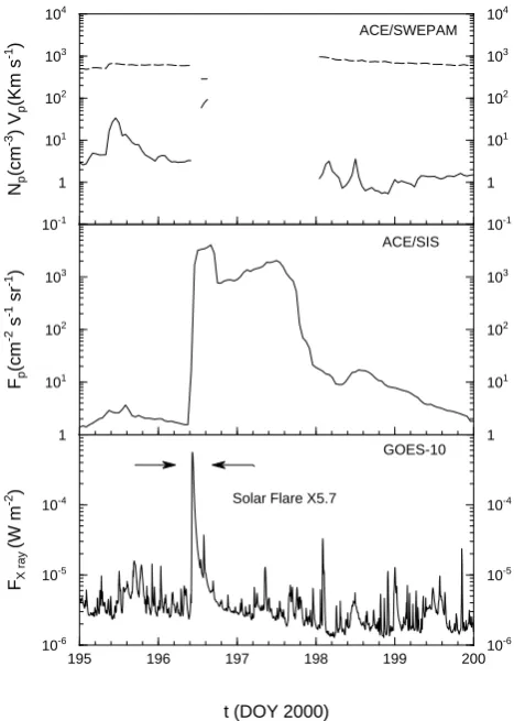
the given time period. All such data gaps occurred after a solar flare and in seven out of nine cases were followed by a geomagnetic storm. This list includes the well-known storms of October 2003, which will be further discussed in Sect. 3.4, and the well-known Bastille event, i.e. 14 July 2000, which we use here to illustrate the relation of SEP (Solar

Ener-10-1 ₁₀-1

1 1

101 ₁₀1

102 ₁₀2

103 ₁₀3

104 ₁₀4

Np

(cm

-3)V

p

(Km

s

-1)

1 1

101 ₁₀1

102 ₁₀2

103 ₁₀3

Fp

(cm

-2

s

-1

sr

-1)

195 196 197 198 199 200

10-6 ₁₀-6

10-5 ₁₀-5

10-4 ₁₀-4

t (DOY 2000)

FX

ray

(W

m

-2)

GOES-10 ACE/SIS ACE/SWEPAM

Solar Flare X5.7

Fig. 1. Upper panel: ACE/SWEPAM proton density (solid line) and

bulk speed (dashed line) hourly averages. Middle panel: ACE/SIS integral proton flux (E>10 MeV) hourly averages. Lower panel: GOES-10 X ray flux five-minute averages (1.0<λ<8.0 ˚A wave-length band).

u1(t)

u2(t)

u₃(t)

O(t+1)

c1(t)

c₂(t)

c3(t)

c4(t)

1

2

4 3

x1(t)

x₂(t)

x₃(t)

x₄(t)

1 input layer

context units

hidden layer output layer

wij(1)

wi(2)

w_ij(c)

recurrent connections

Fig. 2. The Elman scheme used for EDDA.u1,u2andu3are the inputs (normalizedBz,B2andBy2);w0s are the network weights.

The blue lines indicate copying of each hidden layer outputxinto the corresponding context unitc, so thatck(t )=xk(t−1)(see details

in text).

magnetometers are more efficient than plasma instruments in producing continuous time series of data at L1, which are essential for running an operational service devoted toDst

forecasting. On these grounds, it is reasonable to verify the feasibility of aDstforecasting algorithm based on IMF only.

3 The EDDA Model 3.1 The selected network

On the basis of the considerations made in the preceding sec-tion, we trained and tested several networks with different combinations of IMF components. In conclusion, we se-lected for the development of the EDDA algorithm an Elman network (Elman, 1990) with the following structure (Fig. 2):

1. 3 input lines:Bz,B2,By2,

2. 4 context units,

3. 1 hidden layer with 4 neurons, 4. 1 linear output neuron.

In the discussion section we will comment on the signifi-cance of the input choice. The input parameters are hourly averages calculated from L1 IMF data in GSM coordinates. Before being fed into the network, the inputs were nor-malised (see the Appendix for details). The output of the i-th hidden layer neuron is:

xi(t )=tanh( 3

X

j=1

w(_ij1)uj(t )+ 4

X

k=1

w(c)_ik ck(t )), (1)

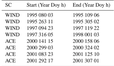
Table 2. The EDDA training set.

SC Start (Year Doy h) End (Year Doy h)

WIND 1995 080 03 1995 109 06 WIND 1995 263 11 1995 305 02 WIND 1997 094 23 1997 119 22 WIND 1997 316 05 1998 001 03 ACE 2000 141 15 2000 158 06 ACE 2000 299 03 2000 324 02 ACE 2001 083 23 2001 125 10 ACE 2001 292 17 2001 307 01

where t is the time in integer hours, the first sum is made over the three normalized external inputsuj(t ), and the

sec-ond one is made over the four context units of contentck(t ). w(_ij1) and w(c)_ik are the weights of the connections between the i-th hidden layer neuron and, respectively, the j-th in-put and the k-th context unit. The context units are defined asck(t )=xk(t−1); in other words, each context unit is

con-nected to the corresponding hidden layer neuron by a recur-rent non trainable connection, whose weight is set constantly to 1, and acts as a memory bank, by receiving at a given time t, the output of the corresponding hidden layer neuron at the preceding time t–1, i.e. one hour earlier. The normalized out-put of the network is obtained from a linear combination of the 4 hidden layer outputs:

O(t+1)=

4

X

i=1

w(_i2)xi(t ), (2)

wherew(_i2)is the weight of the connection between the out-put unit and the i-th hidden neuron. The outout-putOis assigned the timet+1 for inputs at the timet, to account for the 1-h average travel time of the solar wind from L1 to the Earth’s magnetopause.

3.2 The training

The database for developing the EDDA algorithm consists of WIND and ACE IMF hourly averages and of final Kyoto

Dst values from 1995 to 2002 (after 2002 finalDst values

are not available yet), amounting overall to∼64 000 h. The IMF data were collected close to the L1 libration point. From such a database a training set was built, comprising of about 6000 hourly averages from the periods listed in Table 2. The network weightswwere then determined by minimizing the cost function:

E(w)= 1

2

Nt r X

i=1

(T(i)−O(i))2, (3)

andO(i)the corresponding network output. The minimiza-tion ofEis performed in two steps. Firstly, the weights, ini-tially set as small random values, are modified for a prefixed number of iterations by the error backpropagation method (Rumelhart et al., 1986). Then they are perturbed, indepen-dently from one another, by adding a random number ex-tracted from a normal distribution. If this decreases the cost function, the perturbed weights become the new network co-efficients and the process is repeated until theE decrease rate drops below a given threshold. This second step can be viewed as a random walk on the hyper-surfaceEin the space of network weights, where each step is constrained down-hill. As the number of local minima of the cost function is not “a priori” known, it is useful to repeat the training many times, in order to try to explore different attraction basins and hopefully to determine the best local minimum. This hy-brid scheme (a sort of Monte Carlo method) frees the train-ing phase from the bortrain-ing research of the best values for the parameters in the backpropagation (i.e. the learning rate and momentum). Several distinct algorithms were trained and some were retained for further testing, all having very simi-lar performances over the training set.

3.3 The testing

A test set was built by merging together all the periods con-tained in the 1995–2002 database and not previously used during the training. The selected algorithms were run over the whole set and, for each of them, the forecastDsts values

were binned in 25 nT intervals according to the correspond-ing KyotoDst values. On this basis, for each algorithm and

for each bin, a percent root mean square error was calculated as

R(n)=100

s

1 N_bin(n)

PN

(n)

bin

j=1(T(j )−O(j ))2

Tc(n)

, (4)

where n specifies the 25 nT interval, Tc(n) is the

corre-sponding central Dst value, T(j ) and O(j ) are the j-th

Kyoto Dst and algorithm output, respectively, Nbin(n) is the number of data points of the test set whose T(n) falls in the n-th interval. The R parameter provides a quantitative tool to assess the algorithm performance for different geo-magnetic conditions. To this regard, we use the following storm classification: “small” for −50 nT<Dst<−30 nT,

“moderate” for −100 nT<Dst<−50 nT, “intense” for

−200 nT<Dst<−100 nT, “severe” for Dst<−200 nT. The

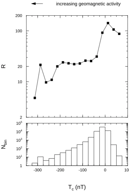
algorithm having the smallest R values for T <−25 nT was chosen as the final EDDA algorithm. For the selected algorithm Fig. 3 displaysRandNbinas a function ofTc, in

the upper and lower panels respectively. TheNbinhystogram approximates the distribution of the Kyoto Dst for the

test set: 94 per cent of the points are concentrated in the

−50 nT<Tc<25 nT interval, but an extended asymmetrical

2 10 20 100 200

R

increasing geomagnetic activity

-300 -200 -100 0 100

1

101

102

103

104

105

Tc(nT) Nbin

Fig. 3. Upper panel: relative errorRfor the EDDA algorithm, as defined in Eq. (4), calculated over the whole test set, and plotted againstTc(see details in text). Lower panel: number of points over which eachRis calculated.

tail extends to negativeDst values.Nbindrops below 10 for Tc<−225 nT, which implies that the last four R values on

the left have little statistical relevance.

Let us first examine the behaviour ofRfor quiet time val-ues of Dst. We see thatR has a maximum of 142 in the

(0,25 nT) binR, and is close to 100 in the two nearby bins and in the (50,75 nT) bin. As far as we can guess, such large relative errors can result from two different contributions: er-rors in theDst baseline, and a failure to reproduce the initial

compression prior to the storm main phase (see also the Dis-cussion section). Moving towards more negativeDst values,

we see thatRdrops to about 30 in the (−50 nT,−25 nT) bin, roughly corresponding to “small” storms; and is fairly con-stant, between 20 and 25, for−225 nT<Tc<−50 nT, i.e. for

“moderate” and “intense” storms. ForTc<−225 nT, i.e. for

110 120 130 140 -300

-200 -100 0 100

Dst

(nT)

YEAR 1998

290 295 300

-300 -200 -100 0 100

YEAR 1999

190 195 200 205 -300

-200 -100 0 100

t (DOY)

Dst

(nT)

YEAR 2000

270 280 290

-300 -200 -100 0 100

t (DOY) EDDA forecast

Kyoto Dst

YEAR 2002

a) b)

c) d)

r=0.889 NMSE=0.247

r=0.971

r=0.965 r=0.920

NMSE=0.080

NMSE=0.083 NMSE=0.156

Fig. 4. Comparison of the EDDADst(red lines) with the KyotoDst

(black lines) for geomagnetically disturbed periods. r is the linear correlation coefficient and NMSE the normalised mean square error (see text for details).

the data displayed in Fig. 3 of Lundstedt et al. (2002). For

−25 nT<Tc<25 nT we found smaller values, in the order

of 83. For −50 nT<Tc<−25 nT, i.e. for “small” storms,

we obtained 32, similar to the EDDA value. Finally, for

−125 nT<Tc<−50 nT, i.e. for “moderate” storms, we found

values between 22 and 25, again similar to the EDDA values. This comparison is based on different data sets for EDDA and “Lund”: as we described earlier, the EDDA test set com-prises of about 58 000 hourly averages, while the data set used for Fig. 3 of Lundstedt et al. (2002) comprises of 40 000 hourly averages. We do not know to what extent the two data sets overlap. As regards to “intense” and “severe” storms, we cannot use R to compare the two algorithms, because: a) Fig. 3 of Lundstedt et al. (2002) stops at Tc=−125 nT;

b) we cannot build an extended common test set for both EDDA and “Lund” in the 1995–2002 period, as we do not know the exact training periods used for the “Lund” algo-rithm. Therefore, forDst<−125 nT, we have to use more

recent data, from 2003 onwards. Unfortunately, after 2002 final KyotoDst values are not available yet and it is not

rea-sonable to base a statistical comparison on provisionalDst

data. Therefore, for such periods, we will only compare the two algorithms for some individual storms (see Sect. 3.4).

Before closing this discussion on the EDDA testing, we notice that in addition toR, it is interesting to consider the EDDA linear correlation coefficient, which is 0.83, and the

total root mean square error

RMSE=

v u u t

1

Ntest Ntest

X

j=1

(T(j )_−O(j )₎2_{, (5)}

which amounts to 13.9 nT over the whole test set (Ntestis the number of test set data points). These values can be directly compared with those quoted by Wu and Lundstedt (1997) for a similar network with the four inputsB, n, V andBs:

0.89 and 16.5. Although the training and testing sets are rather different, also this comparison suggests that the per-formances of the two algorithms are comparable. This and the preceding discussion on the R parameter suggest that, when both plasma and IMF data are available, EDDA pro-duces forecasts at least comparable to those of other “nor-mal” algorithms and, as such, provides a reliable operational forecasting tool.

To show typical examples of the performance of the EDDA algorithm for individual large storms, Fig. 4 com-pares its forecastedDst with the Kyoto Dst index for four

cases of high geomagnetic activity, all pertaining to the test set, i.e. not used in the network training. In each panel the linear correlation coefficientrbetween forecast and observed

Dst, and the normalised mean square error are reported. The

latter is defined as

N MSE=

1 Nev

PNev

j=1(T

(j )_−O(j )₎2

V arev

, (6)

where, for each event,Nevis the number of points andV arev

the variance of the KyotoDst. In the top left hand panelDst

displays a decrease by∼60 nT on day 113, 1998, preceded by an increase by∼20 nT, lasting on the order of 12 h; two further such increases occur on day 121 and on day 122, by

∼40 nT and∼20 nT, respectively; immediately after that, a negative sharp jump, by∼100 nT, occurs on day 122 over a few hours. This is followed by an increase lasting about two days by∼60 nT, followed by the main storm dip to a min-imum value of∼−210 nT on day 124. The recovery phase lasts about 4 days. The EDDADst follows closely the

Ky-otoDst, both during the dips and in the recovery phase; we

notice, however, some minor disagreements, on the order of

∼10–20 nT and the fact that EDDA fails to reproduce the four short-lived increases on days 113, 121 and 122. Such in-creases can be interpreted as due to solar wind compressions prior to the storm main phase. In the top right-hand panelDst

decreases to∼−240 nT on day 295, 1999, to recover over 4 days, while in the bottom left-hand panelDstdisplays several

peaks before a decrease to∼−300 nT on day 198, 2000, and a recovery lasting 2.5 days. In both cases theDst behaviour

is reproduced very well by EDDA, with an exception made again for the short-lived increases just prior to the storm main phase. In the last panel, the KyotoDst displays a broad peak

225 230 235 240 -200

-150 -100 -50 0 50 100

Dst

(nT)

240 242 244 246 248

-200 -150 -100 -50 0 50 100

t (DOY)

Dst

(nT)

Kyoto provisional Dst EDDA

Lund

YEAR 2003

YEAR 2004 ACE verified data

ACE verified data a)

b)

Fig. 5. Comparison of the EDDA (red line) and “Lund”Dst (blue

line) with the KyotoDst (black line) for two “intense” storms.

dip to∼−195 nT on day 274, 2002, and various oscillations during a 10–15 day recovery phase. EDDA reproduces very well all theDst variations, including the compression prior

to the main phase, with an exception made for a difference of∼20 nT observed during day 283 in the recovery phase. As a final remark, we notice that the four cases we have dis-cussed are all rather different from each other, as regarding the strength of the storms and their time scales. In the dis-cussion section we will comment on the compressions prior to the main phase and on the deviations of the order of 20 nT often observed whenDst>−50 nT.

In the Appendix we list all the EDDA weights and normal-isation factors.

3.4 EDDA performance for recent storms

We now apply the EDDA and “Lund” algorithms to more re-cent data, from 2003 onwards, pertaining neither to the train-ing set nor to the test set of either algorithm. We recall that the comparison is made with the provisional KyotoDst as

the finalDst is not available yet.

Figure 5 shows two “intense” storms: that of day 230, 2003, in the top panel, and that of day 243, 2004, in the bottom panel. In both cases the ACE/SWEPAM data do not display any gap, so that the “Lund” algorithm could be

300 302 304 306 308

-500 -400 -300 -200 -100 0 100

t (DOY)

Dst

(nT)

Kyoto provisional Dst EDDA (ACE real-time) Lund (ACE real-time) EDDA (ACE verified) Lund (ACE verified)

YEAR 2003

ACE-SWEPAM plasma instrument saturation

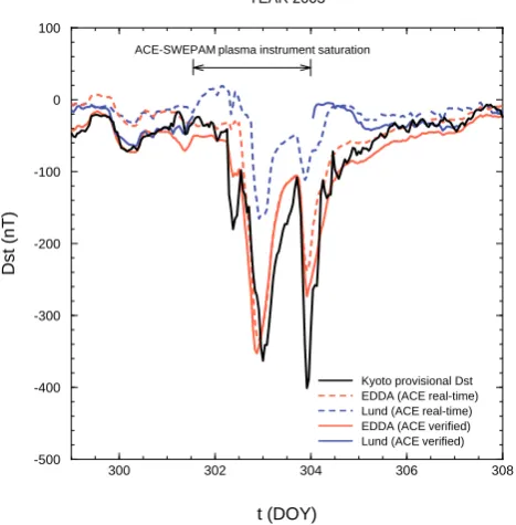
Fig. 6. Performance of the EDDA and “Lund models” (inputs: Bz, Np, Vp) for two storms in October 2003 when the ACE plasma instrument malfunctioned (see details in the text).

run without problems. The Kyoto index is plotted in black, while the EDDA and “Lund” indices are plotted in red and blue, respectively. We see that both EDDA and “Lund” re-produce rather well the KyotoDstfor both storms in all their

phases: the initial compression, the main phase (with minima of∼−170 nT and∼−130 nT in the top and bottom panels, respectively) and the recovery phase. We recall here that in Sect. 3.3 the R parameter showed that “Lund” and EDDA should perform similarly for “small” and “moderate” storms. Figure 5 suggests that this is also true for “intense” storms.

We now turn to discuss a disturbed period when the ACE/SWEPAM instrument malfunctioned for a long time. For that purpose, we consider the well-known “severe” storms observed at the end of October 2003, which have been widely attributed to two CMEs connected to two so-lar fso-lares of magnitudes X17 and X11, occurring one after another. Figure 6 displays the Kyoto provisional Dst

322 323 324 325 326 327 328 -500

-400 -300 -200 -100 0 100

Dst

(nT)

310 312 314 316 318 320

-500 -400 -300 -200 -100 0 100

t (DOY)

Dst

(nT)

Kyoto provisional Dst EDDA

Lund

YEAR 2003

YEAR 2004 ACE verified data

ACE verified data a)

b)

Fig. 7. Comparison of the EDDA (red lines) and “Lund (blue lines)” Dst predictions with the Kyoto provisionalDst index (black line) for two recent storms. In both panels the modelDst is calculated

from ACE verified data.

proton density and bulk flow speed. During the same period the ACE/MAG magnetometer continued to produce reliable data. The incorrect plasma data have been excluded by the ACE/SWEPAM team from the verified final data. For that same time interval, the SOHO CELIAS/MTOF proton mon-itor measured a solar wind speed close to 1100 km/s (i.e. the upper instrumental limit), while the ACE Solar Wind Ion Composition Spectrometer (SWICS) indicated alpha particle speeds in excess of 1900 km/s. This also suggests that the SOHO verified plasma data are not reliable. In this situation, it does not make sense to run the “Lund” algorithm for veri-fied data from 13:00 UT on day 301 to 23:00 UT on day 303. As a consequence, the solid blue line in Fig. 6 has a gap for that time period. On the other hand, we show theDst

fore-casted by the “Lund” model for real time ACE data, to show the effect of the use of incorrect plasma data inputs on theDst

forecast. The “Lund” forecast misses altogether the firstDst

decrease by∼120 nT on day 302; for the first storm it reaches a minimum of−180 nT, to be compared to the−360 nT Ky-oto minimum, while for the second storm it displays a min-imum of−110 nT, to be compared with the−400 nT Kyoto minimum. It is reasonable to argue that the residual corre-lation between the real-time “Lund” forecast and the Kyoto

Dst is due to itsBzinput. As regards to the “Lund” forecast

based on verified data, we notice that it compares reasonably well with the KyotoDst before the data gap. After the gap,

it takes the algorithm almost two days to match again the KyotoDst. As regards to EDDA, we notice that its forecast

based on verified ACE IMF data reproduces rather well the first storm, i.e. the large decrease to∼−360 nT at 00:00 UT on day 303,with an exception made for a 3-h advance. On the other hand, the initialDstdecrease by∼120 nT on day 302 is

only partially reproduced by EDDA. Moreover, EDDA fails to correctly forecast the minimum value ofDst for the

sec-ond storm by 140 nT. In this case the EDDA forecast departs by about 35% from the “real” value, clearly more than the average value of 23 for theRparameter shown in Fig. 3, for

Tc<−50 nT. Finally, we notice that the EDDA “real time”

and the EDDA “verified” forecasts differ by∼20−40 nT for smallDst values. This is due to the fact that real time IMF

data are affected by some errors which are corrected later on by the ACE/MAG team. However, the effects of such errors on the forecastedDst are well below the expected average

relative errors which can be expected from EDDA (see above the discussion over Fig. 3) and are negligible during the main phase of the first large storm.

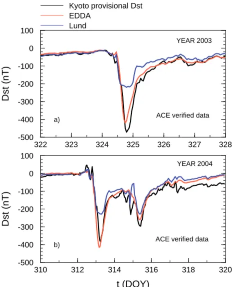
In Fig. 7 we show the EDDA (red lines) and “Lund” (blue lines) performance for two “severe” storms which occurred after October 2003: the November 2003 storm (upper panel) and the November 2004 storm (lower panel). The ACE plasma data appear to be reliable and continuous, with an exception made for one missing data point in the first inter-val. To this regard, we comment that the missing plasma point would have produced a spurious transient in the “Lund” forecast. Actually, we avoided that by interpolating the ACE plasma data before feeding them to the network. In both occasions the Kyoto provisionalDst (black line) displays a

very large negative excursion, below−400 nT. In the Novem-ber 2003 case the Kyoto Dst rises slowly from ∼−40 nT

to∼−30 nT from day 322 to 12:00 UT on day 323, rises to a maximum value of∼−10 nT around 06:00 UT on day 324, undergoes two successive decreases by ∼40 nT over several hours, and then decreases to reach a minimum of

∼−470 nT at 19:00 UT on day 324, followed by a 2–2.5-day recovery. Both “Lund” and EDDA reproduce very well the KyotoDstuntil 10:00 UT on day 324. After that, “Lund”

displays a broad minimum around∼−210 nT, while EDDA drops to∼−420 nT, 50 nT (i.e.∼10%), short of the Kyoto minimum. EDDA follows the Kyoto index during the re-covery phase, while “Lund” displays values larger than the Kyoto Dst by an amount which decreases from ∼100 nT

to ∼10 nT over three days. In the November 2004 case an initial compression is observed on day 312; after the main storm with∼−380 nT minimum, a furtherDst

nega-tive excursion occurs, with∼−300 nT minimum, during the recovery phase. Both “Lund” and EDDA reproduce very well the KyotoDst until the initial compression, which they

of ∼−210 nT, corresponding to the two storms, short of

∼170 nT and∼80 nT, respectively, from the Kyoto minima. On the contrary, EDDA (red lines) reproduces both the first and the second storms, in the first case overestimating the minimum by∼40 nT, and in the second case underestimat-ing it by∼40 nT. However, three smaller dips on day 314 are missed by EDDA.

4 Discussion

Before discussing our findings, first of all, we recall that Wu and Lundstedt (1997) performed a very extensive study of the linear cross-correlation coefficients with different time lags between IMF and plasma parameters, on one hand, andDst,

on the other hand. They considered 9554 h storm time peri-ods, and 1002 h quiet periods and calculated the linear corre-lation withDst for single solar wind parameters and various

functions based on them. We only briefly recall here that they found strong correlations withDst for several functions and

forB, Bs, Bz, andV, while they found a poor correlation for By. Such correlations were stronger for time delays ranging

from one to several hours, depending on the single parameter. These results guided Wu and Lundstedt (1997) and, later on, Lundstedt et al. (2002) in selecting their ANN input parame-ters, including both IMF and solar wind parameters. We have not presented a similar analysis in this work, as we consider these results to be firmly established. However, we remark that the magnetospheric dynamics is thought to be nonlin-early related to the solar wind input, as we already recalled in Sect. 2.1. Actually, this is one of the reasons why ANN is useful for predicting theDst index.

We have taken a different approach to the problem and have chosen to develop an IMF based ANN algorithm. To this regard, we have presented a reasonable argument for our choice in Sect. 2.3, arguing that magnetometers are more re-liable than plasma instruments in terms of continuous tem-poral coverage. As we stated in the Introduction, the aim of this work was to develop an operational ANNDst

algo-rithm based on IMF only, putting a particular emphasis on the reproduction of theDst behaviour for “severe” storms.

The preceding sections show that that task has been accom-plished, as the EDDA algorithm has been extensively and successfully tested over 58 000 h between 1995 and 2002 and over 26 000 h between 2003 and 2005.

We now try to explain how EDDA can predictDst on the

basis of IMF only. In this respect, we recall that magnetic reconnection at the magnetopause and in the tail is, by many authors, considered as an essential process for the transfer of energy, mass and momentum from the solar wind to the mag-netosphere and for energy conversion in the magmag-netosphere itself (Dungey, 1961). Several parameters have been defined and tested over the course of years, to describe the transfer of energy from the solar wind to the magnetosphere. Among them is the Akasofu parameter (Perreault and Akasofu,

1978; Akasofu, 1981), recently reviewed by Koskinen and Tanskanen (2002). This is defined as =V B2sin4(θ/2)l₀2, whereBis the magnitude of IMF,V is the solar wind speed,

θis the IMF clock angle andl0'7 Earth radii. We notice that contains the square of the magnetic field intensity, i.e. the second EDDA input. Moreover,contains theθ clock an-gle, which is determined byBz andBy. Bz is EDDA’s first

input. B_y2was taken as the third EDDA input, becauseByis

known to play a role in the transfer of mass, energy and mo-mentum transfer from the solar wind to the magnetosphere (e.g. Cravens, 1997); since its sign should not be important for such processes, it appears reasonable to have it squared. To comment on the fact that the parameter also depends onV, we notice that this dependance is linear, whereas onB

this dependance is quadratic. This suggests that changes inV

have a smaller impact on the magnetic energy flux carried by the solar wind. However, this point deserves probably further investigation which could be the subject of a future work.

In Sect. 3.3 we compared the EDDA performance with that of the “Lund” algorithm, which, as we already noted, was found in the past to perform better (see Lundstedt et al., 2002) than several algorithms based on differential equations (Burton et al., 1975; Fenrich and Luhmann, 1998; O’Brien and McPherron, 2000). First of all, we made the compari-son from a statistical point of view, finding that “Lund” per-forms somewhat better than EDDA for quiet timeDstvalues,

while the two algorithms are expected to perform in a similar way for “small” and “moderate” storm timeDst values. This

result was extended to “intense” storms by the examination of two cases (see Fig. 5). However, when we compared the two algorithms for four “severe” recent storms (which are a fair sample of the “severe” storms observed between 2003 and 2005), we concluded that EDDA performs better: for the October 2003 two storms, the “Lund” forecasts, based on real time data, fail because the plasma data provided by ACE/SWEPAM are wrong (Fig. 6); for the November 2003 and 2004 storms “Lund” largely fails to match the minima of both storms (Fig. 7). With regard to such different perfor-mances we can make the hypothesis, that they depend on the different training sets used for the two algorithms, but cannot test this hypothesis as we do not know the exact time periods used for the “Lund” training.

In the last part of this section we wish to comment on mi-nor limitations of the EDDA algorithm, which we have al-ready pointed out in the preceding sections. First of all, we recall the second of the October 2003 storms (see Fig. 6), which occurred during the recovery phase of a preceding storm. In this case we remarked a relative error of 35 per-cent on theDst minimum. The probable reason for this poor

2004 in Fig. 7). The reason for such different performances is a matter for future investigation.

We now turn to the differences often observed between the Kyoto index and the forecasted index for smallDst values

(cf. Sect. 3.3). As quiet periods account for the great major-ity of data points, the ultimate effect of such differences is the increase in the total RMSE and of the high values of theR pa-rameter forDst>−25 nT, as already discussed with reference

to Fig. 3. Actually, high values for such parameters, in the order of 100, are commonly quoted for all past algorithms, as it can be seen in Fig. 3 of Lundstedt et al. (2002) and in Table 1 of Wang et al. (2003). In this respect, several con-siderations can be made. First of all, we recall that the pro-duction of theDst index requires subtracting out a fairly big Sqionospheric current system contribution. This subtraction is imperfect and leaves a residual signal (Temerin and Li, 2002). Moreover, it must be considered that the unperturbed value of the horizontal component of the geomagnetic field is not exactly known, but it is only estimated through the an-nual average of theDst values calculated from the 5 quietest

days observed at each station during every month. It is plau-sible, then, that the determination of the baseline can be, in certain circumstances, an error source for the prediction of smallDst absolute values. In fact, we observe in the test data

set periods of very low geomagnetic activity, also lasting ten days, when the predictedDst is constantly lower or higher,

on the order of 20 nT, than the observed one. Actually, the uncertainties in the determination ofDst are one of the

ma-jor concerns of all authors attempting to develop algorithms for its forecast (e.g. see the discussion made by Temerin and Li, 2002).

To conclude this section, we briefly comment on the EDDA performance during the initial compression of the magnetosphere prior to the main storm phase. It is accepted that such a compression be produced by the solar wind dy-namic pressure (mostly density) increase. Therefore, it is reasonable that the EDDA algorithm fails to reproduce such a compression, as it does not include among its inputs nei-ther the solar wind density nor its speed. We have noted that this seems to happen, to different extents, for the majority of the storms described in this paper. However, this does not occur for the storms of day 274, 2002, day 229, 2003, and day 243, 2004. We have already noticed in Sect. 3.3 that the large value of the parameterR for small values of

Dst could be due in part to this effect. We note, however,

as we recalled already, that large values of the RMS and of theR parameter for smallDst values are also quoted for

al-gorithms which include the plasma parameters among their inputs (see, e.g. Fig. 3 of Lundstedt et al., 2002) and (Table 1 of Wang et al., 2003). Moreover, “Lund”” and EDDA be-haved in the same way during the initial compression for the three examples discussed in Sect. 3.4. A more detailed dis-cussion of this issue goes beyond the purpose of this paper.

5 Summary

We described EDDA, a new Elman Artificial Neural Net-work, trained over ∼6000 hourly averages of WIND and ACE data. EDDA calculates theDst index on the basis of

IMF data only and is, therefore, capable of issuing opera-tional forecasts based on the current real time ACE L1 IMF data. The EDDA performance was carefully examined over an extended test period from 1995 to 2002. Moreover, its per-formance was checked for the recent “severe” geomagnetic storms which occurred between 2003 and 2005, for which provisional, but not final,Dst data are available. Moreover,

it was shown that the EDDA performance is in general com-parable to that of similar algorithms which also make use of plasma data, although a failure to fully reproduce the initial compression prior to the storm main phase may occur. It was also shown that the EDDA ability to forecast theDst index

based on IMF only has an undoubted operational advantage in all circumstances (very interesting in the framework of space weather) when the predictions of algorithms based on both IMF and plasma parameters fail because the solar wind speed exceeds the upper limit of the L1 plasma instruments or large radiation, and SEP fluxes cause temporary faults in such instruments.

Finally, we suggested that the three magnetic inputs of the EDDA model, namelyBz, B2, By2, which closely recall the

information contained in the Akasofuparameter, can catch, especially in enhanced geomagnetic activity conditions, the large majority of the relevant information necessary to de-scribe the relationship between the solar wind trigger and the

Dst index.

Appendix A

The EmpiricalDst Data Algorithm

The EDDA algorithm can be implemented through a com-puter programme performing the following steps.

1) setc=(0.0,0.0,0.0,0.0)T

2) get first or next input dataBz,B2,By2

3) computeu=( u1, u2, u3)T = Bz

Nr1, B2 Nr2,

By2

Nr3

T

4) computex=tanh(w(1)u+w(c)c)

5) computeDst =Nr4w(2)x 6) setc=x

7) goto 2

At the beginning the context units are unknown and are set to 0. Depending on solar wind conditions, it takes from a few hours to 1–2 days for EDDA to reach normal operation. The same occurs in the case of data gaps.

1 h and thebsymbol denotes high time resolution IMF GSM data.

In step 3 the inputs are divided by the normalisation fac-torsNr1,Nr2andNr3, so that the network operates on adi-mensional inputs. Similarly, in step 5 the network output is multiplied by the normalisation factorNr4. This is common practice with neural networks (see, e.g. Wu and Lundstedt, 1997). The four normalisation factors were obtained by cal-culating the maxima of the absolute values of the correspond-ing parameters over the period 1995–2002 for the OMNI data set.

The EDDA weights and normalization factors are:

w(1)= 

 

−0.00863 0.25861 −0.03929 0.00387 −0.04102 −0.01309

−0.05323 0.01495 −0.03294

−0.00418 −0.03920 −0.01922



 

w(c)= 

 

0.29238 0.07855 0.05065 0.15604 0.10092 0.88728 0.03804 0.11780 0.28768 0.01891 0.76351 0.07686 0.56835 0.15990 0.05034 0.11086



 

w(2)=(−0.08588 −0.00006 −2.02734 −0.07205)

Nr1=44.7 nT, Nr2=(48.2)2(nT)2,

Nr3=(34.3)2(nT)2, Nr4=387.0 nT.

Acknowledgements. The authors would like to thank the ACE

spacecraft team and SEC for making the real time and verified data available, and the WIND, GOES, SOHO spacecraft teams and NSSDC for making their datasets available, too. This work was par-tially supported by the ESA contract N. 17032/03/NL/LvH, in the framework of the Pilot Project on Space Weather Applications.

Topical Editor T. Pulkkinen thanks M. Temerin and another ref-eree for their help in evaluating this paper.

References

Akasofu, S. I.: Prediction of development of geomagnetic storms using the solar wind-magnetosphere energy coupling function, Planet. Space Sci., 29, 1151–1158, 1981.

Burton, R. K., McPherron, R. L., and Russell, C. T.: An empirical relationship between interplanetary conditions and Dst, J. Geo-phys. Res., 80, 4204–4214, 1975.

Consolini, G. and Chang, T. S.: Magnetic Field Topology and Criti-cality in Geotail Dynamics: Relevance to Substorm Phenomena, Space Sci. Rev., 95, 309–321, 2001.

Cravens, T. E.: Physics of Solar System Plasmas, Cambridge Uni-versity Press, Cambridge, UK, 1997.

Dungey, J. W.: Interplanetary Magnetic Field and the Auroral Zones, Phys. Rev. Lett., 6, 47–48, 1961.

Elman, J. L.: Finding structure in time, Cognitive Sci., 14, 179–211, 1990.

Fenrich, F. R. and Luhmann, J. G.: Geomagnetic response to mag-netic clouds of different polarity, Geophys. Res. Lett., 25, 2999– 3002, 1998.

Gonzalez, W. D. and Echer, E.: A study on the peak Dst and peak negative Bz relationship during intense geomagn etic storms, Geophys. Res. Lett., 32, 18 103–18 106, 2005.

Gonzalez, W. D., Joselyn, J. A., Kamide, Y., Kroehl, H. W., Ros-toker, G., Tsurutani, B. T., and Vasyliunas, V. M.: What is a geomagnetic storm?, J. Geophys. Res., 99, 5771–5792, 1994. Gonzalez, W. D., Tsurutani, B. T., and Cl´ua de Gonzalez, A. L.:

Interplanetary origin of geomagnetic storms, Space Sci. Rev., 88, 529–562, 1999.

Gosling, J. T.: The solar flare myth, J. Geophys. Res., 98, 18 937– 18 950, 1993.

Kane, R. P.: How good is the relationship of solar and interplanetary plasma parameters with geomagnetic storms?, J. Geophys. Res., 110, 2213–2215, 2005.

Klimas, A. J., Vassiliadis, D., Baker, D. N., and Roberts, D. A.: The organized nonlinear dynamics of the magnetosphere, J. Geophys. Res., 101, 13 089–13 114, 1996.

Koskinen, H. E. J. and Tanskanen, E. I.: Magnetospheric energy budget and the epsilon parameter, J. Geophys. Res., 107, A11, doi:10.1029/2002JA009283, 2002.

Lundstedt, H., Gleisner, H., and Wintoft, P.: Operational fore-casts of the geomagnetic indexDstindex, Geophys. Res. Lett., 29(24), 2181, doi:10.1029/2002GL016151, 2002.

O’Brien, T. P. and McPherron, R. L.: Forecasting the ring current index Dst in real time, J. Atmos. Terr. Phys., 62, 1295–1299, 2000.

Perreault, P. and Akasofu, S.-I.: A study of geomagnetic storms, Geophys. J., 54, 547–573, 1978.

Rumelhart, D. E., Hinton, G. E., and Williams, R. J.: Learning rep-resentations by back-propagating errors, Nature, 323, 533–536, 1986.

Temerin, M. and Li, X.: A new model for the prediction of Dst on the basis of the solar wind, J. Geophys. Res., 107, A12, 1472, doi:10.1029/2001JA007532, 2002.

Wang, C. B., Chao, J. K., and Lin, C. H.: Influence of the solar wind dynamic pressure on the decay and injection of the ring current, J. Geophys. Res., 108, A9, 1341, doi:10.1029/2003JA009851, 2003.

Watari, S., Kunitake, M., and Watanabe, T.: The Bastille Day (14 July 2000) Event in Historical Large Sun-Earth Connection Events, Solar Phys., 204, 425–438, 2001.

Wu, J. and Lundstedt, H.: Geomagnetic storm predictions from so-lar wind data with the use of dynamic neural networks, J. Geo-phys. Res., 102, 14 255–14 268, 1997.