University of Trento
Department of Physics
Thesis
Submitted to the
Doctoral School in Physics
by
Matteo Leonardi
In candidature for the degree of
Philosophiae Doctor - Dottore di ricerca
Development of a squeezed
light source prototype
for Advanced Virgo
Tutor: Prof. Giovanni Andrea Prodi
Co-Tutor: Prof. Jean-Pierre Zendri
Contents
Introduction v
I
Theory
1
1 Gravitational wave and detectors 3
1.1 Gravitational waves . . . 3
1.2 GW detector: Advanced Virgo . . . 5
1.3 Gravitational wave detection . . . 9
2 Classical and quantum optics 13 2.1 Quantization of the electromagnetic field . . . 13
2.1.1 Fock states . . . 14
2.1.2 Coherent states . . . 15
2.1.3 The Heisenberg uncertainty principle . . . 15
2.1.4 Squeezed states . . . 16
2.2 Linearized quantum theory . . . 16
2.2.1 Photodetection . . . 17
2.2.2 Balanced homodyne detection . . . 18
2.3 Squeezed state and losses . . . 19
2.3.1 Squeezing ellipse phase fluctuations . . . 20
2.4 Non linear optics . . . 21
2.4.1 Phase matching . . . 23
2.5 Squeezed state generation . . . 24
3 Squeezing applied to GW detectors 25 3.1 Squeezing applied to AdV . . . 25
II
Experiment
31
4 Advanced Virgo squeezed vacuum source 33 4.1 Squeezed vacuum source optical layout . . . 334.1.1 Mach-Zehnder (MZ) . . . 35
4.1.2 Infrared mode-cleaner (MCIR) . . . 39
4.1.3 Balanced homodyne detector . . . 43
4.2 Controls and electronics . . . 47
4.2.1 Phase one: Labview based controls and custom PLL and DDS . . . 48
4.2.2 Phase two: AdV compatible controls and electronics . . . 50
5 Second Harmonic Generator 55 5.1 SHG requirements . . . 55
5.2 Mechanics . . . 57
5.3 Double pass measurements . . . 58
5.3.1 Multimode SHG . . . 61
5.4 In cavity SHG . . . 65
5.4.1 Alignment and mode matching . . . 67
5.4.2 High efficiency SHG . . . 68
5.4.3 Competitive non linear processes . . . 73
5.4.4 Birefringence and absorption losses . . . 76
6 Faraday Isolator 79 6.1 Polarizers’ polarization quality . . . 81
6.1.1 Experimental setup . . . 85
6.1.2 Virgo+ INJ FI polarizer . . . 85
6.1.3 EOT polarizer . . . 88
6.1.4 INJ IPC polarizer . . . 90
6.1.5 Polarizers’ summary . . . 92
6.2 Thermal design . . . 92
6.3 In vacuum Faraday Isolator . . . 95
A Optical simulation 101 A.1 Second Harmonic Generator . . . 101
A.1.1 Analytic results . . . 101
A.1.2 Finesse simulation . . . 103
Conclusions 105
Acknowledgements 109
Introduction
A century after the prediction of the existence of gravitational waves by A. Einstein and after over fifty years of experimental efforts, gravitational waves have been detected at Earth directly [1, 2]. This result is a major achievement and opens new prospectives for the exploration of our universe. Gravitational waves carry different and complementary information about the source with respect to electromagnetic signals. In particular the first detection demonstrated the existence of stellar-mass black holes, binary systems of black holes and their coalescence.
The detection was made by the LIGO instruments which are twin kilometer-scale Michel-son interferometers in the US. These detectors represent the second generation of gravitational wave interferometers and, for the first time, they achieved the outstanding strain sensitivity of 10−23Hz−1/2 between 90 Hz and 400 Hz. In the next months the LIGO network will be joined by another second generation detector: Advanced Virgo located near Pisa, Italy. The sensitivity of these advanced detectors is set by different noise sources. In particular, in the low frequency range (below 100 Hz) major contributions come from thermal noises, gravity gradient noise and radiation pressure noise; instead, the high frequency band (above 100−200 Hz) is dominated by shot noise. Quantum noise (radiation pressure and shot noise) is expected to dominate the detector sensitivity in the whole frequency band at the final target laser input power.
To decrease the shot noise while increasing the radiation-pressure noise, or vice-versa, Caves [3] proposed in 1981 the idea of the squeezed-state technique. The LIGO collaboration demon-strated for the first time in 2011 [4] that the injection of a squeezed vacuum state into the dark port of the interferometer can reduce the shot noise due to the quantum nature of light. This result was achieved with the German-British interferometer GEO600 and was replicated in 2013 with the LIGO interferometer at Livingston [5]. After these results, the LIGO collaboration have pursued further the research in the squeezed-state technique [6, 7, 8] which is considered mandatory for third generation of ground based interferometric detectors.
In 2013, the Virgo collaboration started developing the squeezed-state technique. The subject of my thesis is the realization of a prototype of frequency independent squeezed vacuum state source to be injected in Advanced Virgo. This prototype is developed in collaboration with other Virgo groups.
This thesis is organized as in the following. In Chapter 1 I give an overview of gravitational wave and ground based interferometric detectors. In Chapter 2 I summarize the results of the theory of non linear optics of interest for the development of a squeezed vacuum source for Advanced Virgo. In chapter 3 I discuss the expected Advanced Virgo performances including the use of squeezed-state technique. In the second part of this work I describe my experimental work: in Chapter 4 I describe the prototype under development, in Chapter 5 the second harmonic generator and in Chapter 6 the Faraday isolator.
The darker the night, the brighter the stars.
Crime and Punishment, Fyodor Dostoevsky, 1866
Part I
Theory
Chapter 1
Gravitational wave and detectors
This chapter provides a brief introduction to gravitational waves (GW) and to the main GW sources accessible by ground based detectors. The second part reviews the optical-interferometric detectors for GW, focusing in particular on Advanced Virgo (AdV).
1.1
Gravitational waves
Gravitational waves are ripples in the space time. They are a special solution of the Einstein equations for weak gravitational field.
The Einstein equations can be written as (see [9]):
Rik−
1 2gikR=
8πG
c4 Tik (1.1.1)
or alternatively
Rik=
8πG
c4
Tik−
1 2gikT
(1.1.2)
whereRikis the Ricci curvature tensor,gikis the metric tensor,Gis the Newton’s gravitational
constant, Tik is the stress-energy tensor, R is the scalar curvature and Rii =R=−
8πG
c4 T with
T =Ti
i.
In the vacuum space,Tik= 0 and the Einstein equations reduce to
Rik= 0 (1.1.3)
Having a weak gravitational field means that the metric tensor can be expressed as a small perturbation to the Minkowski metricηik:
gik=ηik+hik (1.1.4)
wherehik is the small perturbation. In this situation of weak gravitational field,
Rik=
1
2hik (1.1.5)
whereis the D’Alembert operator: =−ηlm∂x∂l∂x2 m = ∆−
1
c2
∂2
∂t2 Considering eq(1.1.5) with eq(1.1.3), choosing the Lorenz gauge and the transverse traceless gauge, we find
hik= 0 (1.1.6)
This equation is formally equivalent to the electromagnetic wave equation. Gravitational fields, like electromagnetic fields, propagate at the speed of light. Their properties can be derived from eq(1.1.6). All the details can be found in any general relativity textbook [9].
The gravitational waves are transverse waves which polarization is defined by a symmetric rank two tensor . The two polarization are usually identified as h+ and h×; these differ from
each other by aπ/4 rotation in the plane perpendicular to the propagation direction.
Gravitational waves are emitted by accelerated masses. The lowest multipole term which can radiate a gravitational wave is the quardupole term. This means that mass distributions that exhibit a spherical symmetry cannot radiates GWs.
Examples of GWs sources of interest to ground based detectors are:
• Compact binary systems: [10] these systems are formed by two compact stars such as neutron stars or black holes orbiting around their center of mass. As demonstrated by Hulse and Taylor on a binary neutron star pulsar system, PSR B1913+16, massive binary rotating systems lose energy via GW radiation [11, 12, 13]. Up to coalescence, the frequency and the amplitude of the emitted GW increase as the orbit radius decrease. This results in a chirp signal.
• Spherical asymmetric spinning massive objects: these objects can be non-symmetric pulsars and neutron stars. The expected GW signal from this source is a continuous signal, whose frequency is proportional to the source rotating frequency. The GW signal strength increases as the degree of axial-asymmetry increases.
• Stochastic background: [14] in analogy to cosmic microwave background (CMB), also a cosmic gravitational wave background is expected as remnant of the Big Bang. Unlike the CMB that gives information of approximately 300000 years after the Big Bang, the stochastic background can give information from about 10−36s after the Big Bang. In addition other GW backgrounds are expected from the overposition of many astrophysical emitters.
• Supernovae: [15, 16] stellar explosions that are not spherical symmetric are predicted to emit GWs.
Figure 1.1: Effect of the two GW polarization on two rings of free falling test particles. The top strip shows the effect of an h+ polarized GW while the bottom one shows the effect of an h×
1.2. GW DETECTOR: ADVANCED VIRGO 5
The effect of a gravitational wave on an extended body is a modification of the relative distances between different positions. Fig.1.1 shows the effect of the two polarisations (h+ and
h×) of a passing gravitational wave on two rings of free-falling test particles.
The strength of a GW is usually measured in strain, that is the fractional length change it induces:
h=δL
L (1.1.7)
where δL is the length variation induced by the GW and L is the original length. The largest astrophysical events are expected to have strains of the order of h= 10−21.
1.2
GW detector: Advanced Virgo
The GW ground based detectors that have the highest sensitivity are the GW interferometric detectors. These detectors are based on the Michelson interferometer design.
Figure 1.2: Basic scheme of a Michelson interferometer. The laser light is splitted at the beam-splitter and then, after traveling through the arms, it’s recombined again at the beam beam-splitter. The light detected at the photodetector carries the information of the relative displacement of the two end mirror. In this case, the two end mirrors are displaced by anh+ polarized GW.
Fig.1.2 shows the basic scheme of a Michelson interferometer. The two end mirrors are displaced due to the passage of an h+ polarized GW. The light detected at the photodetector carries the information of the relative displacement δLof the two mirrors.
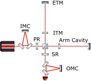
cleans the beam from spurious TEM modes and from control sidebands. Fig.1.3 shows the basic scheme of a GW interferometer.
IMC
OMC
SR
PR
Arm Cavity
ITM
ETM
Figure 1.3: Basic scheme of a GW interferometric detector. In the figure IMC is the input mode cleaner, PR is the power recycling mirror, SR the signal recycling mirror, OMC is the output mode cleaner and each arm cavity is formed by the input test mass (ITM) and the end test mass (ETM). The length of the arm cavity isLarm ≈3 km for AdV and Larm ≈4 km for the two
aLIGO.
In the near future, the network of ground based GW interferometric detectors will comprise the two LIGO detectors (LIGO Livingston and LIGO Hanford, both in the US), the Virgo col-laboration detector (near Pisa, Italy), KAGRA detector (in Japan, at Kamioka), GEO-HF (near Hannover, Germany) and LIGO-India (joint India-US detector recently approved). Last year, in September, the first two second generation GW detectors (the two LIGO) started collecting science data, showing a strain sensitivity of≈10−23/√Hz within 100−500Hz. The italian-french AdV detector is currently under construction and will join the world wide network before the end of this year.
In the following I detail the sensitivity curve expected for AdV pointing out the major noise sources. All the details of the following discussion can be found in [17, 18].
AdV is expected to reach the design sensitivity of≈3×10⁻²⁴/√Hz between 50−400Hz. To reach this goal, a four steps upgrade process is planned by implementig the following configura-tions:
• power recycled,Pin= 25 W;
• dual recycled,Pin= 25 W, tuned signal recycling;
1.2. GW DETECTOR: ADVANCED VIRGO 7
• dual recycled,Pin= 125 W, detuned signal recycling.
The input powerPinis measured after the IMC anddual recycled refers to the presence of both
the PR and the SR mirrors.
Frequency [Hz]
101 102 103
Strain [1/
Hz]
10-24 10-23 10-22
AdV Noise Curve: Pin = 125.0 W
Quantum noise Gravity Gradients Suspension thermal noise Coating Brownian noise Coating Thermo-optic noise Substrate Brownian noise Seismic noise Excess Gas Total noise
Figure 1.4: Dual recycled AdV noise curve with 125 W input power and tuned SR mirror. The simulation is performed using GWINC code.
Fig.1.4 shows an example of the expected noise budged of a dual recycled AdV with 125 W input power and tuned SR mirror. The sensibility of the GW detector is limited by several noise source for different frequency ranges.
Thermal noise
A motion of the reference surface of the test masses due to brownian motion can mimic the signal of an incoming GW. The two most limiting noises within this class are the coating brownian thermal noise and the suspension thermal noise (see Fig.1.4). The first arises from the brownian noise of the test masses coating, while the second is mainly due to the silica fibers that suspend the input test masses (ITMs) and the end test masses (ETMs). This noise can be reduced either improving the quality of the coating and fiber materials or heading to low temperature operations. Additional thermal noise sources come from thermo-optical processes in the coating, Brownian motion of the mirror substrate, thermo-elastic processes of the substrate and thermo-refractive processes in the output mode cleaner (OMC).
Seismic noise
Frequency [Hz]
10-1 100 101 102
Seismic motion [m/ Hz
1/2
]
10-12 10-11 10-10 10-9 10-8 10-7 10-6 10-5
50-th percentile 75-th percentile 90-th percentile 99-th percentile
Figure 1.5: Horizontal ground motion measured on the floor of the AdV central building during science run VSR4 (see [19]) in the West direction.
Gravity gradient noise
This noise arises from the Newtonian gravitational attraction between masses, in particular between the detector test masses and nearby moving masses. Those moving masses can be either people, cars, trains, etc and also environmental density changes (e.g. atmospheric pressure, subterranean sediment settlement). This is one of the most tricky noise source of the ground based GW detectors and probably the hardest low frequency noise to be tackled. In AdV is expected to limit the sensitivity below 20−30 Hz. Underground detectors can reduce the impact of this noise source, as e.g. KAGRA, and future third generation GW detectors.
Quantum noise
This noise source arises from the quantum nature of light. It is composed by the photon counting noise (phase noise or shot noise) at the photodetector and by the radiation pressure noise (that is the photon momentum transfer at the test masses). For the AdV case, the shot noise will limit the sensitivity for all the frequency above≈300Hz while the radiation pressure noise will contribute to limit the low frequency sensitivity. This noise cannot be reduced in the whole frequency range by a brute force approach. The most promising approach is to build correlations between the shot noise and the radiation pressure noise in order to reshape the quantum noise. A method to build those correlation is to utilize a signal recycling technique. Another method is to substitute the coherent vacuum flactuation that enters from the dark port of the interferometer with a squeezed vacuum, in order to reduce one of the two quantum noises at the price of enhancing the other one. Since the shot noise and the radiation pressure noise limit the interferometer sensitivity in two different frequency ranges, the optimal solution is to inject a frequency dependent squeezed vacuum state whose ellipse rotates as function of frequency in order to reduce the radiation pressure noise at low frequency and the shot noise at high frequency.
The aim of the project which provides the framework for this thesis is to realize a squeezed vacuum source for AdV.
Other noises
1.3. GRAVITATIONAL WAVE DETECTION 9
1.3
Gravitational wave detection
On 14 September 2015 the first gravitational wave have been directly observed by the two LIGO observatories (LIGO Hanford and LIGO Livingston) [1]. This gravitational wave was originated by a coalescence of two black holes at a luminosity distance of distance of 410+160−180Mpc corresponding to a redshift z = 0.09+0−0..0304. In the source frame, the initial black hole masses are 36+5−4M and 29+4−4M, and the final black hole mass is 62
+4
−4M, with the equivalent of 3.0+0−0..55Menergy radiated in gravitational waves. These observations demonstrate the existence
of gravitational wave, the existence of stellar-mass black holes with masses higher than 20M, the
existence of binary stellar-mass black hole systems and that those binary systems can coalesce. Fig.1.6 shows the coincident signal GW150914 detected by the two LIGO observatories.
Figure 1.6: From [1]. The gravitational-wave event GW150914 observed by the LIGO Hanford (H1, left column panels) and Livingston (L1, right column panels) detectors. Times are shown relative to September 14, 2015 at 09:50:45 UTC. For visualization, all time series are filtered with a 35−350Hz bandpass filter to suppress large fluctuations outside the detectors’ most sensitive frequency band, and band-reject filters to remove the strong instrumental spectral lines. Top row, left: H1 strain. Top row, right: L1 strain. GW150914 arrived first at L1 and 6.9+0−0..54ms later at H1; for a visual comparison, the H1 data are also shown, shifted in time by this amount and inverted (to account for the detectors’ relative orientations). Second row: Gravitational-wave strain projected onto each detector in the 35−350Hz band. Solid lines show a numerical relativity waveform for a system with parameters consistent with those recovered from GW150914 [20] confirmed to 99.9% by an independent calculation based on [21]. Shaded areas show 90% credible regions for two independent waveform reconstructions. One (dark gray) models the signal using binary black hole template waveforms [22]. The other (light gray) does not use an astrophysical model, but instead calculates the strain signal as a linear combination of sine-Gaussian wavelets [23, 24]. These reconstructions have a 94% overlap, as shown in [22]. Third row: Residuals after subtracting the filtered numerical relativity waveform from the filtered detector time series. Bottom row: A time-frequency representation [25] of the strain data, showing the signal frequency increasing over time.
ob-served by the GW detectors network [2]. The signal, GW151226, persisted in the LIGO frequency band for approximately 1 s, increasing in frequency and amplitude over about 55 cycles from 35 to 450 Hz, and reached a peak gravitational strain of 3.4+0−0..79 ×10−22. The inferred source-frame initial black hole masses are 14.2+8−3..37M and 7.5+2−2..33M, and the final black hole mass is
20.8+6−1..17M. At least one of the component black holes has spin greater than 0.2. This source is
located at a luminosity distance of 440+180−190Mpc corresponding to a redshift of 0.09+0−0..0304.
1.3. GRAVITATIONAL WAVE DETECTION 11
Chapter 2
Classical and quantum optics
In this chapter I briefly overview the basics of non linear optics and quantum optics which are prerequisites for the thesis work. The electromagnetic field quantization and Heisenberg Uncertainty are used to introduce properties of coherent squeezed states and to the homodyne detection method to characterize them. Non linear media are discussed in the context of second harmonic generation and squeezed light generation.
2.1
Quantization of the electromagnetic field
The quantization of the electromagnetic field usually starts from the classical Hamiltonian of the field, that is:
H= 1 2
Z
V
dτ
0E2+
B2
µ0
(2.1.1)
where the integration is performed over the volume of the electromagnetic field and E is the electric field, 0 is the vacuum dielectric constant and B is the magnetic field and µ0 is the vacuum magnetic permeability. Following [28], this Hamiltonian can be rewritten as
H= 1 2
X
j
mjωj2q
2
j+
p2
j
mj
!
(2.1.2)
where mj is a constant with the dimension of mass, ωj is the electromagnetic field angular
frequency, qj is the normal amplitude with the dimension of a length and pj = mjq˙j is the
canonical momentum ofqj.
The quantization of this Hamiltonian can be realized identifyingqjandpj as operators which
obey the commutation relations:
[qj, pj0] =ı~δ(j−j0) and [qj, qj0] = [pj, pj0] = 0 (2.1.3)
Making the canonical transformation to operatorsaj anda†j defined as follows
aj =
eıωjt
p
2mj~ωj
(mjωjqj+ıpj) (2.1.4a)
a†j = e
−ıωjt
p
2mj~ωj
(mjωjqj−ıpj) (2.1.4b)
the Hamiltonian (2.1.2) becomes
H=~
X
j
ωj
a†jaj+
1 2
(2.1.5)
Using (2.1.3) the commutation relations betweenaj anda†j are
[aj, a†j0] =δ(j−j0) and [aj, aj0] = [a†j, a†j0] = 0 (2.1.6)
The operatorsaj and a†j are usually addressed as the annihilation and the creation operators,
respectively.
Starting from the annihilation and the creation operators of a single mode field, we define the quadrature operatorsX+ andX−:
X+= a+a†
and X−=−ı a−a† (2.1.7)
These two quadrature operator are usually called amplitude quadrature and phase quadrature [29]. A generic quadrature operatorXθ can be described using a linear combination ofX+ and
X−:
Xθ=ae−ıθ+a†eıθ
=X+cosθ+X−sinθ (2.1.8)
whereθis the quadrature angle. Starting from (2.1.6) it is straightforward to demonstrate that
[X+, X−] = 2ı (2.1.9)
Another useful operator is the number operator defined as
N =a†a (2.1.10)
Taking the mean number of photon of a statehNiand multiplying by the photon energy~ω we have the optical power of the state
Popt=hNi~ω (2.1.11)
2.1.1
Fock states
Fock or number states are eigenstates of the number operator:
N|ni=n|ni (2.1.12)
The ground state or vacuum state is defined as
N|0i= 0 (2.1.13)
Combining eq.(2.1.5) and (2.1.13) we can calculate the energy of the vacuum state. We take the case of a single mode field.
h0| H |0i=1
2~ω (2.1.14)
2.1. QUANTIZATION OF THE ELECTROMAGNETIC FIELD 15
Starting from the vacuum state all the Fock state can be defined applying the creation operator. In general we have
|ni= a
†n
√
n! |0i (2.1.15)
The Fock states are orthogonal and complete:
hn|mi=δnm and
∞
X
n=0
|ni hn|= 1 (2.1.16)
The variances of the quadrature operators on a Fock state are:
V(X+) = (∆X+)2=hn|(X+)2|ni −(hn|X+|ni) 2
= 1 + 2n (2.1.17)
and
V(X−) = (∆X−)2=hn|(X−)2|ni −(hn|X−|ni)2
= 1 + 2n (2.1.18)
In the case of the vacuum state ∆X+= ∆X− =±1.
2.1.2
Coherent states
An example of a coherent state is the light emitted by a stabilized and monochromatic laser. A coherent state|αiis a left eigenstate of the annihilation operator:
a|αi=α|αi (2.1.19)
whereαis a complex number. The mean photon number of a coherent state is therefore
hα|N|αi=|α|2 (2.1.20)
and ∆N=|α|. This is characteristic of a Poissonian distribution.
Starting from the vacuum state, a coherent state can be defined using a displacement operator
D(α):
|αi=D(α)|0i with D(α) = exp αa†+α∗a
(2.1.21)
The variances of the quadrature operators on a coherent state areV(X+) =V(X−) = 1 and
therefore ∆X+= ∆X− =±1.
2.1.3
The Heisenberg uncertainty principle
The Heisenberg uncertainty principle [30] states that for two noncommuting Hermitian operators
qandpone cannot simultaneously measure their physical quantities with arbitrary precision:
∆q∆p≥ 1
2|h[q, p]i| (2.1.22)
Heisenberg uncertainty principle applied to the quadrature operators (eq.(2.1.9)) translates into
∆X+∆X−≥1 (2.1.23)
From the previous two paragraph we see that all coherent states and vacuum state fulfill the special case of the Heisenberg uncertainty principle
∆X+∆X−= 1 (2.1.24)
2.1.4
Squeezed states
The Heisenberg uncertainty principle states that the product of the variances of two noncom-muting operators has a minimum. However, it does not put any constrain on the individual component variances, thus if
(∆q)2< 1
2|h[q, p]i| or (∆p) 2< 1
2|h[q, p]i| (2.1.25)
but not simultaneously, the state is said to be squeezed.
In analogy to the coherent state, a squeezed state can be described applying a squeezing operator to a vacuum state. The squeezing operatorS(r, θ) is defined as
S(r, θ) = exp
1
2re
−2ıθ(a)2−1 2re
2ıθ(a†)2
(2.1.26)
where r is the the squeezing factor and θ is the quadrature angle of the squeezing: θ = 0 corresponds to amplitude squeezing andθ=π/2 to phase squeezing.
The squeezed vacuum is thus obtained applying the squeezing operator to the vacuum state
|0, r, θi=S(r, θ)|0i (2.1.27)
while a bright squeezed state is defined as
|α, r, θi=D(α)S(r, θ)|0i (2.1.28)
For an amplitude squeezed state (θ= 0), application of the number operator will yield
hα, r,0|N|α, r,0i=|α|2+ sinh2(r) (2.1.29)
On the same state, the variance of the quadrature operatorsX+ andX− are
(∆X+)2= e−2r and (∆X−)2= e2r (2.1.30)
On the other hand, for a phase squeezed state (θ=π/2) the variance of the quadrature operators
X+ andX− are
(∆X+)2= e2r and (∆X−)2= e−2r (2.1.31)
The squeezed state described previously are minimum uncertainty states. Imperfect processes, such as loss, will result in a state that is not a minimum uncertainty state. We therefore can define the squeezing purityP as
(∆X+)2(∆X−)2=P (2.1.32)
A pure state will have a purity of P = 1, as does the vacuum. A pure state is a minimum uncertainty state.
2.2
Linearized quantum theory
Let’s consider the single mode annihilation operatoraand let’s break into two different contri-butions:
a=α+δa(t) (2.2.1)
2.2. LINEARIZED QUANTUM THEORY 17
The number operator becomes
N =a†a= (α∗+δa†(t))(α+δa(t))
≈α2+α(δa†(t) +δa(t))
≈α2+αδX+(t) (2.2.2)
where we have taken the arbitrary phase of α real and linearized by assuming the fluctuation are small and hence neglecting higher than first order terms in the fluctuations. We see that we are effectively measuring the quadrature operatorδX+(t) =δa†(t) +δa(t). For this reasonδX+ is referred to as the amplitude quadrature operator.
2.2.1
Photodetection
Combining eq.(2.2.2) with eq.(2.1.11) we have that the optical power of a beam can be written as
Popt≈~ω(α2+αδX+(t)) (2.2.3)
A common measurement of the optical power of a beam involves a photodiode. As a consequence of the Photoelectric Effect, incident photons hitting a photosensitive medium are a source of freely moving electrons. The produced photocurrenti, is given by
i=ρPopt=
eηpd
~ω Popt (2.2.4)
whereρis the responsivity of the photodetector (in units of A/W),ηpdis the quantum detection
efficiency of the detection medium,~ωthe energy per photon, andeis the modulus of the electron charge. Using eq.(2.2.3) in eq.(2.2.4) in the case of an ideal photodiode (ηpd= 1) we have
i≈e(α2+αδX+(t)) (2.2.5)
The first term of eq.(2.2.5) is a non-fluctuating term that is directly proportional to the optical intensity of the incident light, while the second term is a fluctuating term proportional to the amplitude quadrature times the coherent amplitude.
pd
'
Figure 2.1: Model of a real photodiode with quantum efficiencyηpd. One of the two input power
of the beam splitter is occupied by the input beam, while the other is occupied by the vacuum state. The light that reaches the ideal photodiode is a linear combination of the two input of the beam splitter.
The case ofηpd<1 can be modeled considering a beam that go through a beam splitter with
detected by the ideal photodiode is the linear combination of the two beam splitter input beams, that are the beam that we want to measure and the vacuum. In this case, the photocurrent generated by the photodiode is
i≈eηpdα2+eα
ηpdδX+α(t) +
q
ηpd(1−ηpd)δX+v(t)
(2.2.6)
The photocurrent in this case differs by eq.(2.2.5) in both the fluctuating and the non-fluctuating term: the non-fluctuating term is scaled by the quantum efficiency of the photodiode and the fluctuating term is a linear combination between the amplitude quadrature fluctuation of the input beam (δXα
+(t)) and the amplitude quadrature fluctuation of the vacuum state (δX+v(t)).
2.2.2
Balanced homodyne detection
As seen in the previous paragraph, non perfect quantum efficiency is a limitation to the measure-ment of quantum noises of light. Measuring the quantum noise requires that all classical noise terms, such as laser intensity noise and electronic noise, are reduced to a level well below the noise level of interest. To perform these measurements, a commonly used method is the balanced homodyne detection (see Fig.2.2).
bs
signal
local
oscillator
C
D
A
B
pd
1pd
2Figure 2.2: Scheme of an ideal balanced homodyne detector. The local oscillator (LO) and the signal beams are mixed on the beam splitter. The two resulting beams are detected by two ideal photodiodes pd1and pd2.
The two inputs of the homodyne detector are the signal beam A = α+δa and the local oscillator (LO) beamB=β+δb. The quantum properties of the signal beam are measured by recording the difference of the two photodiodes’ photocurrents.
The two output beams of the beam splitter (CandD) are
C=p1−ηbsA+
√
ηbsBeıθ (2.2.7a)
C=√ηbsA−
p
1−ηbsBeıθ (2.2.7b)
whereηbsis the splitting ratio of the beam splitter and θ is the relative phase of the two input
beams and it has been chosen to ensure that the coherent amplitude terms of the fields are real. Assuming ideal photodiodes, the two photocurrents are
i1/e= (1−ηbs)A†A+ηbsB†B+
p
ηbs(1−ηbs) A†Beıθ+B†Ae−ıθ
(2.2.8a)
i2/e=ηbsA†A+ (1−ηbs)B†B−
p
ηbs(1−ηbs) A†Beıθ+B†Ae−ıθ
2.3. SQUEEZED STATE AND LOSSES 19
and the difference of the two photocurrent is
(i1−i2)/e= (1−2ηbs)A†A+ (2ηbs−1)B†B+ 2
p
ηbs(1−ηbs) A†Beıθ+B†Ae−ıθ
(2.2.9)
Using eq.(2.2.2) we can approximate A†A ≈ α2+αδXA
+ and B†B ≈ β2 +βδX+B where
δXA
+ = δa+δa† and δX+B =δb+δb† are the amplitude quadrature of the signal and the LO beam respectively. Therefore, eq.(2.2.9) can be approximate as follow:
(i1−i2)/e≈(1−2ηbs)(α2+αδX+A) + (2ηbs−1)(β2+βδX+B) + 2
p
ηbs(1−ηbs)×
2αβcosθ+α(δX+Bcosθ−δX
B
−sinθ) +β(δX
A
+cosθ+δX
A
−sinθ)
(2.2.10)
In most of the cases of interest, the LO is much brighter than the signal field (β α). This condition is particularly true when the signal beam is a vacuum state. In those cases, all the terms of eq.(2.2.10) whereβ is not present can be neglected. Therefore we have that
(i1−i2)/e≈(2ηbs−1)(β2+βδX+B)+
2pηbs(1−ηbs)
2αβcosθ+β(δX+Acosθ+δX−Asinθ) (2.2.11) Supposing an ideal splitting ratio of 50% we finally have
(i1−i2)/e≈2αβcosθ+β(δX+Acosθ+δX
A
−sinθ) (2.2.12)
The first term of eq.(2.2.12) is a DC term that describes the interference between the two fields as the phase between the signal and the local oscillator is varied. The second term contains the quantum properties of the signal beam that are amplified by the coherent amplitude of the LO beam. By choosing the phase between the signal and the LO to beθ= 0, the output of the homodyne detector is proportional to the signal amplitude quadrature, while choosing θ=π/2 the output is proportional to the signal phase quadrature.
2.3
Squeezed state and losses
In section 2.2.1 we shown how in the non ideal case of a photodiode, the quantum properties of a state are mixed with the quantum properties of the vacuum state. In general, any losses (such as transmission losses, absorption, non ideal quantum efficiency, mode mismatching, etc) can be modeled with the introduction of a partially reflective beam splitter which couples the vacuum state noises into the beam quantum properties. After the virtual beam splitter we will have
a0 =√ηa+p1−ηδv (2.3.1)
where 1−ηare the generic “losses” and henceηis the transmittivity of the virtual beam splitter. Therefore we also have
a0†a0=η(α2+αδX+a) +pη(1−η)αδX+v (2.3.2) whereδXv
+ is the vacuum amplitude quadrature fluctuation and the input beam is linearized as did in the previous sections. The variance of the photon numberVa0 can be calculated as
Va0 =ηVa+ (1−η)Vv (2.3.3)
being Va the photon number variance of the state before the beam splitter and Vv the photon
number variance of the vacuum state. SinceVv= 1 andη∈[0,1], the higher are the losses, the
closer isVa0 toVv.
For a squeezed state the variance of the two quadratureX+ and X− are given respectively
Losses (1-η)
0 0.1 0.2 0.3 0.4 0.5 0.6 0.7 0.8 0.9 1
Quadratures variance [dB]
-15 -10 -5 0 5 10 15
Figure 2.3: Effect of losses on a pure amplitude/phase squeezed state. For an amplitude squeezed state the continue lines represent the variance of X+ and the dashed lines are the variance of
X−; for a phase squeezed state the variances are just switched. The X+ and X− quadrature
variances are plotted as a function of the losses in three different situations: red curves refer to a state with 15 dB of amplitude/phase noise suppression and 15 dB of phase/amplitude noise enhancement in the loss-less case; blue (green) curves show the same information for a state with 10 dB (5 dB) squeezing in the loss-less case.
2.3.1
Squeezing ellipse phase fluctuations
Another effect that decreases the noise enhancement/suppression of a squeezed state is the cou-pling of the X+ and X− quadrature variances due to the squeezing ellipse phase fluctuations.
As function of the rms phase fluctuations ¯θ, the measured variances are
V(X+0,−) =V(X+,−) cos2θ¯+V(X−,+) sin2θ¯ (2.3.4)
Losses (1-η)
0 0.1 0.2 0.3 0.4 0.5 0.6 0.7 0.8 0.9 1
Phase fluctuation [mrad]
0 10 20 30 40 50 60 70 80 90 100
Squeezing level [dB]
-14 -12 -10 -8 -6 -4 -2
Figure 2.4: Degradation of the squeezing level of a pure 15 dB squeezed state due to the combined effect of losses and squeezing ellipse phase fluctuations.
2.4. NON LINEAR OPTICS 21
the degradation of the squeezing level starting from a pure 15 dB squeezed state.
2.4
Non linear optics
The beginning of the field of non linear optics is often taken to be the discovery of second-harmonic generation by Franken et al.(1961) [31], shortly after the demonstration of the first working laser by Maiman in 1960.
For most of the materials the induced polarizationP(t) depends linearly on the strengthE(t) of an applied optical field:
P(t) =0χ(1)E(t) (2.4.1)
where χ(1) is the linear susceptibility and0 is the permittivity of free space. In general, this approximation does not hold true. In fact, for intense electric field, eq(2.4.1) is generalized by expressing the polarization P(t) as a power series in the field strengthE(t):
P(t) =0
h
χ(1)E(t) +χ(2)E2(t) +χ(3)E3(t) +. . .i
≡P(1)(t) +P(2)(t) +P(3)(t) +. . . (2.4.2)
The quantitiesχ(2) andχ(3) are known as the second- and third-order nonlinear optical suscep-tibilities, respectively. In my work only second-order processes are present.
Let’s take the case where the electric field can be written asE(t) =E0e−ıωt+ c.c. In this case, the second-order polarization of eq.(2.4.2) is
P(2)(t) =0χ(2)
E02e−2ıωt+ c.c.+0χ(2)
2E0E∗0
(2.4.3)
This equation lead to the production of two different field, one at twice the frequency of the input electric field and one at zero frequency. The two processes involved in this situation are known as second harmonic generation (SHG) and optical rectification (OR) respectively. If the input electric field is composed by two or more frequency components, the second-order nonlinear optical susceptibility leads also to sum and difference frequency generation (SFG and DFG respectively).
z
L
1
2
3
=
1
+
2
d
=
eff
(2)
1
2
Figure 2.5: Sum-frequency generation.
Let’s take the case of SFG. Fig.2.5 shows the scheme of the process. The generic wave equation for nonlinear optical media can be written as in [32]:
∇2E
n−
(1)(ω
n)
c2
∂2E
n
∂t2 =
1
0c2
∂2PN L
n
whereEn is the electric field of the n-th mode,ωn is the angular frequency of the mode,PN Ln
in the nonlinear part of the polarization and(1)(ω
n) is the linear part of the relative
permit-tivity, which is different for each material. This equation holds true for the case of an isotropic, dissipationless material.
For simplicity, let’s take the case of plane wave propagating in the +zdirection. In this case, the inputs and the output beams of Fig.2.5 can be written as:
Ei(z, t) =Eieıωit+ c.c. where Ei=Aieıkiz (2.4.5)
withi= 1,2,3. We also write the nonlinear source term appearin in eq(2.4.4) as
P3(z, t) =P3eıω3t+ c.c. where P3= 40def fE1E2 (2.4.6)
havingdef f =χ(2)/2.
Without going into details, combining eqs(2.4.4), (2.4.6) and (2.4.5) in the slowly varying amplitude approximation, we end up with three coupled differential equations that describes the spatial dependences ofAi:
dA1 dz =
2ıdef fω21
k1c2
A3A∗2e
−ı∆kz (2.4.7a)
dA2 dz =
2ıdef fω22
k2c2
A3A∗1e−ı∆kz (2.4.7b)
dA3 dz =
2ıdef fω23
k3c2
A1A2eı∆kz (2.4.7c)
where ∆k=k1+k2−k3 which is called the wavevector mismatch. Eqs(2.4.7) can be solved in the simplified case of no-pump depletion, that means thatA1andA2can be taken as constants. In this situation, for ∆k= 0, the amplitude A3 increases linearly with z, and consequently its intensity increases quadratically withz. When the ∆k= 0 condition is not fulfilled, eq(2.4.7a) can be solved by direct integration (betweenz= 0 andz=L):
A3(L) =
2ıdef fω23A1A2
k3c2
Z L
0
eı∆kzdz= 2ıdef fω 2 3A1A2
k3c2
eı∆kL−1
ı∆k
(2.4.8)
The intensity of the generated wave is given by the magnitude of the time-averaged Poynting vector, which is given by
Ii= 2ni0c|Ai|2 i= 1,2,3 (2.4.9)
We thus obtain
I3=
8n30d2ef fω34|A1|2|A2|2
k2
3c3
eı∆kL−1
∆k 2 (2.4.10)
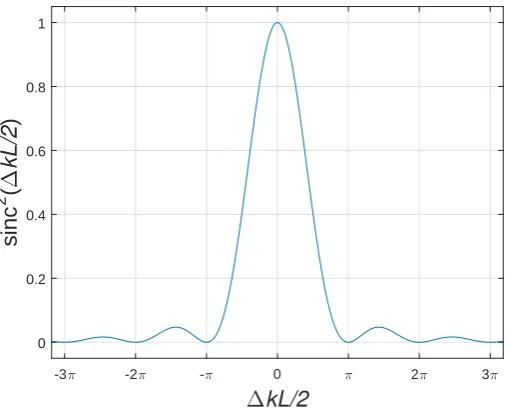
Note that the effect of wavevector mismatch is entirely included in the squared modulus term. This term can be rewritten as
eı∆kL−1
∆k 2
=L2sinc2(∆kL/2) (2.4.11)
2.4. NON LINEAR OPTICS 23
∆
kL/2
-3π -2π -π 0 π 2π 3π
sinc
2
(
∆
kL/2
)
0 0.2 0.4 0.6 0.8 1
Figure 2.6: Effect of wavevector mismatch on the sum frequency generation efficiency.
2.4.1
Phase matching
The phase matching condition is a general condition that does exist not only for SFG (and therefore for SHG) but also for DFG. This condition is usually not easy to achieve. That’s because, commonly, materials shows an effect known as normal dispersion: the refractive index increases as function of frequency. Therefore, the condition for perfect phase matching with
collinear beams n
1ω1
c +
n2ω2
c =
n3ω3
c (2.4.12)
where ω1+ω2 = ω3 cannot be achieved. The most common procedure for achieving phase matching is to make use of the birefringence displayed by many materials. Birefringence is the dependence of the refractive index on the direction of polarization of the optical radiation.
Three different techniques are commonly used to perform the phase matching. The first two described make use of the birefringence, while the third allows the phase matching condition to be fulfilled even for non birefringent materials:
Type I phase matching: the two input fields (atω1andω2) have the same polarization and the produced field is orthogonally polarized. This can be achieved by adjusting the angle of incidence, changing the crystal temperature or both. The phase matching is said to be noncritical if the refractive indices are matched for light fields propagating in the plane which is orientated 90◦ with respect to the optical axis of the crystal.
Type II phase matching: the two input fields (atω1 andω2) have orthogonal polarization and the harmonic field has the same polarization as one of the fundamental fields. Again this can be achieved by adjusting the angle of incidence, changing the crystal temperature or both. Independently of the relative values ofω1andω2, type I phase matching is easier to achieve than type II.
in a phase mismatch of
∆kQP M =k1+k2−k3− 2π
Λ (2.4.13)
where Λ is the crystal inversion period. Due to the periodic poling term, there is no requirement of the refractive index being equal for the fundamental and harmonic fields. An advantage of the periodic poled (PP) materials is that phase matching can be achieved at room temperature over a very wide temperature range compared to the other two phase matching methods and the phase matching temperature depends on Λ. Periodically poling allows to exploit additional terms of the nonlinear susceptibility matrix which are larger than those used in type I and type II phase matching. Using quasi-phase matching, the constantdef f of eqs(2.4.7) must be substituted withdQP M = (2/π)def f.
2.5
Squeezed state generation
The very first generation of a squeezed state was realized in 1985 by Slusher et al. [33] using nondegenerate four-wave mixing. The actual most commonly used process to generate a squeezed state is the degenerate parametric down conversion in an optical cavity, as used firstly by Wu et al. in 1986 [34]. The degenerate parametric down conversion is a particular case of DFG where the pump field atω3=ωp create via nonlinear interaction a signal field atω1=ω2=ωs=ω3/2 (see [32]).
In the rotating wave approximation, the Hamiltonian of a degenerate parametric down con-version process can be written as in [28]:
H=~κ(a†a†b+aabdagger) (2.5.1)
wherea, a†andb, b†are the annihilation/creation operators for the signal field and the pump field respectively andκis a constant which depends upon the second-order susceptibility tensor that mediates the interaction. Let’s assume the pump field is a coherent state and let’s approximateb
asβexp(−ıφ) whereβis the real amplitude of the pump field andφis the relative phase between the pump and the signal beams. In this case, eq(2.5.1) can be rewritten as
H=~κβ(a†a†e−ıφ+aaeıφ) (2.5.2)
The evolution operator associated to this process is therefore
Chapter 3
Squeezing applied to GW
detectors
In this chapter I describe the advanced Virgo simulated noise budget with the injection of a squeezed vacuum into the dark port of the interferometer.
Injecting a squeezed vacuum state into an interferometer, modifies the quantum noises of the detector with respect to the case where no squeezing is injected. A detailed explanation of the quantum noises of a GW interferometer can be found in [35]. The injection of frequency independent squeezed vacuum into a GW interferometer have already demonstrated to reduce the detector shot noise [4, 5].
3.1
Squeezing applied to AdV
The tool developed by the LIGO-Virgo collaboration to compute the expected noise budget for a GW detector is called GWINC. According to [17], the detector design sensitivity will be achieved following a step by step process. Within this process, three different interferometer configurations are identified:
1. Power recycled interferometer: in this situation the power recycling (PR) mirror is installed while the signal recycling mirror (SR) is not. This is the first step foreseen by the AdV collaboration and will be implemented with an input power of 25 W.
2. Tuned dual recycled interferometer: both the two recycling cavities (PR and SR) are installed in this configuration and the signal recycling cavity is tuned.
3. Detuned dual recycled interferometer: the only difference of this configuration from the one previous is that the signal recycling cavity is detuned. The choice of the detuning angle allows to tailor the spectral sensitivity of the detector.
Since the squeezing injection is expected to impact only on the quantum noises of the inter-ferometer, in the following, all the non quantum noises are considered altogether and shown as one overall contribution.
Within the collaboration, the sensitivity of the detectors is usually expressed in observable ranges for specific GW sources, in units of Mpc. This quantity expresses the expected maximum distance at which an emitted GW can be measured with a SNR≥8. The two more common GW signals that are used to compute ranges are the emission from the coalescence of two neutron
stars (NS) with mass MN S = 1.4M and the coalescence of two black holes (BH) with mass
MBH = 30M.
The expected NSNS and BHBH ranges for AdV in the various configuration as function of the input power and the signal recycling mirror detuning are shown in the following, using optimization routines that I developed to post-process the results from the GWINC code.
P
in[W]
0 20 40 60 80 100 120 140
NSNS range [MPc]
101 102 103 104 105 106 107 108 109 110 M NS=1.4Msun P in[W]
0 20 40 60 80 100 120 140
BHBH range [MPc]
200 300 400 500 600 700 800 900 1000 1100 M BH=30Msun
MBH=25Msun M BH=20Msun M BH=15Msun M BH=10Msun
MBH= 5Msun
Figure 3.1: Binary coalescences ranges for configuration 1 as function of the input power. The NSNS range increases as function of input power, while, for black holes of massMBH = 30Mthe
detection range decrease as the input power increases. For BH with small masses, this behavior changes and forMBH = 5M, the same behavior of the NSNS ranges is obtained.
Fig.3.1 shows the expected ranges for NSNS and BHBH coalescence as function of the injected power (10−125 W): the NSNS ranges increases as function of the injected power reaching the maximum of 109.7 Mpc withPin = 125 W. On the other hand, the BHBH range forMBH =
30M decreases as the input power increases and the maximum range is 1078 Mpc withPin=
10 W. This difference is entirely due to the fact that the radiation pressure noise gets higher as the input power increases and this spoils the detector low frequencies performances. Fig.3.2 shows the AdV sensitivity curves in this two cases.
Frequency [Hz] 101 102 103 Strain [1/ Hz] 10-24 10-23 10-22 10-21
AdV Noise Curve: Pin = 125.0 W
Sensitivity curve Non quantum noises Quantum noises Frequency [Hz] 101 102 103 Strain [1/ Hz] 10-24 10-23 10-22 10-21
AdV Noise Curve: Pin = 10.0 W
Sensitivity curve Non quantum noises Quantum noises
Figure 3.2: The sensitivity curves I computed for configuration 1 in the case of Pin = 125 W
(left) andPin= 10 W (right) are shown.
For configuration 2 and 3 I computed the binary system ranges (in this caseMBH = 30M) as
3.1. SQUEEZING APPLIED TO ADV 27
of the dual recycled interferometer as function of the input power and the SR detuning. The best NSNS range (145.6 Mpc) is obtained withPin = 125 W and a SR detuning of 0.2565 rad,
that is 14.69◦ and the best BHBH range (1381 Mpc) is obtained with Pin = 10 W and a SR
detuning of 1.282 rad, that is 73.47◦. As in the configuration 1 case, the difference between this two sets of parameters are the low frequency performances of the interferometer.
P
in [W]
20 40 60 80 100 120
SR cavity detuning [deg]
0 60 120 180 240 300 360
NSNS range [MPc]
20 40 60 80 100 120 140 P
in [W]
20 40 60 80 100 120
SR cavity detuning [deg]
0 60 120 180 240 300 360
BHBH range [MPc]
200 400 600 800 1000 1200
Figure 3.3: Binary coalescences ranges for a dual recycled interferometer as function of the input power and the SR detuning, configurations 2 and 3
Frequency [Hz] 101 102 103 Strain [1/ Hz] 10-24 10-23 10-22 10-21
AdV Noise Curve: P
in = 125.0 W
Sensitivity curve Non quantum noises Quantum noises Frequency [Hz] 101 102 103 Strain [1/ Hz] 10-24 10-23 10-22 10-21
AdV Noise Curve: P
in = 10.0 W
Sensitivity curve Non quantum noises Quantum noises
Figure 3.4: The sensitivity curves for configuration 3. (left) input power and SR tuning are optimized to maximize the NSNS range: Pin = 125 W and SR detuning is 0.2565 rad; (right)
input power and SR tuning are optimized to maximize the BHBH range: Pin= 10 W and SR
detuning is 1.282 rad.
squeezing working group set a challenging but not optimistic target for the squeezing input losses equal to 20%. Those losses take into account the OPO escape efficiency and absorption, Faraday isolators transmission losses, mode matching between the squeezed vacuum and the interferometer, OMC absorption and mode matching, AdV photodetector non perfect quantum efficiency. For the phase noise a conservative value equal to 30 mrad has been chosen as target.
Squeezing level [dB]
0 5 10 15
Squeezing angle [deg]
0 30 60 90 120 150 180
NSNS range gain
0.3 0.4 0.5 0.6 0.7 0.8 0.9 1
Squeezing level [dB]
0 5 10 15
Squeezing angle [deg]
0 30 60 90 120 150 180
BHBH range gain
0.3 0.4 0.5 0.6 0.7 0.8 0.9 1 1.1 1.2
Figure 3.5: NS (left) and BH (right) coalescence ranges gain for configuration 1 withPin= 25 W
as function of the frequency independent squeezing level and angle.
Fig.3.5 shows the ranges gain for configuration 1 withPin= 25 W as function of the squeezing
level and the squeezing angle. The ranges are normalized on the ranges obtained with the same configuration and input power but without squeezing injection. For both the NS and BH ranges, the squeezing injection enhance the interferometer sensitivity. In particular, the NSNS range has a maximum of 113.1 Mpc with an injection of 3.6 dB of squeezing and a squeezing angle of 62.1◦, while, for BHBH range, a maximum of 1183 Mpc is achieved with the injection of 7.8 dB of squeezing at a squeezing angle of 86.9◦. These two ranges are higher compared to the best ranges obtained with configuration 1 without any squeezing injection. It is worth to notice that injecting a phase squeezed state at a squeezing angle close to 90◦means that we are injecting an amplitude squeezed vacuum state.
The result of injecting a frequency independent phase squeezed vacuum state in an interfer-ometer in configuration 2 (that is dual recycled interferinterfer-ometer with tuned signal recycling cavity) is an enhancement of both the NSNS and BHBH ranges with respect to the ranges obtained in the same configuration but without squeezing. An example forPin= 25 W is in Fig.3.6.
In all the previous cases, the ranges are maximized without considering that this maximization usually spoils the high frequency performances of the interferometer. To increase the BHBH and NSNS ranges injecting a squeezed vacuum state while preserving the high frequency performances of the detector, frequency dependent squeezing must be taken into account.
3.1. SQUEEZING APPLIED TO ADV 29
Squeezing level [dB]
0 5 10 15
Squeezing angle [deg]
0 30 60 90 120 150 180
NSNS range gain
0.4 0.5 0.6 0.7 0.8 0.9 1 1.1 1.2
Squeezing level [dB]
0 5 10 15
Squeezing angle [deg]
0 30 60 90 120 150 180
BHBH range gain
0.4 0.5 0.6 0.7 0.8 0.9 1 1.1
Figure 3.6: Binary ranges for configuration 2 with Pin = 25 W. The highest ranges are:
is a frequency dependent squeezed vacuum. This cavity is usually calledfilter cavity (FC). To obtain a squeezed ellipse optimal rotation for a GW interferometer, two filter cavities are needed [36].
The study of the injection of a frequency dependent squeezed vacuum into a GW interfer-ometer is not the aim of my work. However, as a view into future developments for a GW detector with squeezing, I computed the sensitivity curve for the particular case of the injection of 10 dB of frequency dependent squeezing with optimal angle rotation into a configuration 2 interferometer withPin= 125 W (see Fig.3.7).
Frequency [Hz]
101 102 103
Strain [1/
Hz]
10-24
10-23 10-22 10-21
AdV Noise Curve: P
in = 125.0 W
Optimal rotation freq. dependent squeezing Non quantum noises
Quantum noises No squeezing
One FC freq. dependent squeezing
Figure 3.7: AdV noise budged in configuration 2 withPin= 125 W with the injection of different
types of frequency dependent squeezing. The light blue curve is the AdV noise budget without any squeezing injection, the orange curve is the noise budget with the injection of a non optimal frequency dependent squeezing (as can be realized with just one FC) and the black curve is the noise budget with the injection of a frequency dependent squeezing with optimal ellipse rotation. The blue curve is the noise contribution due to the sum of all non quantum noises; the red curve is the noise contribution due to the sum of quantum noises in the case of frequency dependent squeezing with optimal ellipse rotation.
The better is enemy of the good.
Proverbi italiani, Orlando Pescetti, 1603
Part II
Experiment
Chapter 4
Advanced Virgo squeezed vacuum
source
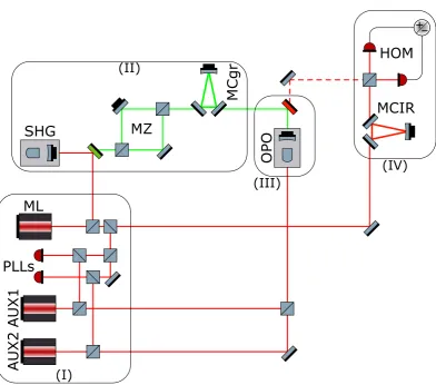
This chapter describes the optical layout along with the electronics and controls of the AdV squeezed vacuum source, with special focus on the parts which I worked on during this thesis. The realization of the first AdV squeezed vacuum source is a collaborative effort involving many italian Virgo laboratories: INFN Napoli, INFN Roma1 (LaSapienza) and INFN Roma2 (TorVergata), INFN Pisa, INFN Genova, INFN Padova-Trento. My group, Padova-Trento, delivered some key subsystems as the Second Harmoic Generator, the Phase Locked Loops, Infrared Mode Cleaner and took a wider responsibility on the implementation of controls and on the integration of the several parts.
Considering the results of the LIGO and GEO600 experiments [4, 5], the collaboration decided to set the following requirements:
• 12 dB frequency-independent squeezed vacuum in the AdV detection band (that is between 10 Hz and 10 kHz). This requirement is as produced, i.e. before measurement losses.
• 10 mrad rms phase noise
• up to 5% losses without taking into account the measurement losses.
4.1
Squeezed vacuum source optical layout
The optical layout of the squeezed vacuum source is schematized in Fig.4.1. The setup can be divided into four main blocks:
Laser sources: it contains three IR laser sources and two phase locked loops (PLL). The main laser (ML) is used to pump the second harmonic generator and to provide the local oscillator for the homodyne detector. The first auxiliary laser (AUX1) provides the coherent control field used to stabilize the squeezed ellipse angle, while the second auxiliary laser (AUX2) is used as the optical parametric oscillator (OPO) length control beam. Two PLLs lock the phase of the two auxiliary laser to the main laser, each one with a different frequency detuning.
Second harmonic source: this block contains a second harmonic generator (SHG), a Mach-Zehnder interferometer (MZ) and a triangular cavity (MCgr). The SHG provides the green
SHG
MZ
MCgr
OPO
MCIR
HOM
ML
A
UX1
A
UX2
PLLs
(II)
(I)
(III)
(IV)
4.1. SQUEEZED VACUUM SOURCE OPTICAL LAYOUT 35
pump power for the OPO, while the MZ stabilizes the pump power and the MCgr stabilizes the phase of the pump field at high frequency1and defines the mode shape.
Squeezed light source: it contains the OPO cavity. This cavity, driven below threshold, generates the squeezed vacuum state of light.
Squeezed light detector: this block contains a triangular cavity (MCIR) and the homodyne detector (HOM). The MCIR is used to clean and define the mode shape of the HOM local oscillator and the HOM is used to characterize the produced squeezed vacuum state.
The Napoli group was in charge to develop the Mach-Zehnder interferometer and the green mode cleaner, the Roma1 group developed the homodyne electronic board, the Roma2 group was in charge to realize the OPO cavity, the Pisa group provided a DSP board and the Padova-Trento group was in charge to realize the second harmonic cavity, the infrared mode cleaner and to develop all the electronics and controls needed in the optical bench.
The SHG is fully described in Chapter 5. Here I describe the other main parts of the squeezed vacuum source. The controls of the optical system are described in Section 4.2. Here I just anticipate that two versions of the controls and electronics were implemented during this work and which I callphase one andphase two.
Fig.4.2 shows a picture of the squeezed vacuum source optical bench as it was at the beginning of May 2016.
4.1.1
Mach-Zehnder (MZ)
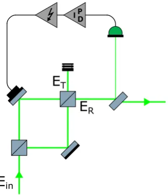
The Mach-Zehnder (MZ) interferometer is used to stabilize the power of the green pump to a fixed value. This is needed since a fluctuation of the green pump will lead to a fluctuation of the degree of produced squeezing. Fig.4.3 (left) shows a photo of this setup: it was produced by INFN-NA and I took care of its characterization and control. The MZ consists of two high reflectivity mirrors and two beam splitters.
Fig.4.3 (right) shows the scheme of the electric fields in the MZ interferometer: Ein is the
input electric field. Referring to this picture,ER andET can be written as
ER=
r1r2−t1t2e2πı
∆L
λ +φ
Ein
ET =ı
r1t2+t1r2e2πı
∆L
λ +φ
Ein (4.1.1)
where r1 and r2 are the amplitude reflectivities of the first and the second beam splitter re-spectively,t1 andt2are the amplitude transmittivities of the first and the second beam splitter respectively, ∆Lis the length difference of the two interferometer paths,λis the light wavelength andφis the difference of the Gouy phases of the two beams at the recombination point.
Usually the contribution of the Gouy phase can be neglected; in particular, it is negligible when ∆L zR where zR is the Rayleigh length of the beam. This term becomes important
when the interferometer has length unbalanced arm or if the beam is heavily focused. Our MZ is not in such situations, so in the following we can neglect the Gouy phase contribution.
Our MZ has beam splitters’ power reflectivities2 R
1 = R2 = 0.1 for p-polarized light and
R1 = R2 = 0.01 for s-polarized light. Fig.4.4 shows the MZ total power reflection and power
1A cavity acts as a low pass filter with a frequency cut equal to the half of its FWHM. Therefore the MCgr
stabilizes the phase of the green pump field for frequency greater than the half of its FWHM.
2Remind that
R=|r|2 and R+T+ Σ = 1
4.1. SQUEEZED VACUUM SOURCE OPTICAL LAYOUT 37
E
inE
r1
E
RE
TE
t1r
1,t
1r
2,t
2Figure 4.3: (left) Picture of the installed MZ. (right) Working principle scheme of the MZ
2π∆L/λ[rad]
0 π 2π 3π 4π RMZ
0.6 0.65 0.7 0.75 0.8 0.85 0.9 0.95 1
2π∆L/λ[rad]
0 π 2π 3π 4π TMZ
0 0.05 0.1 0.15 0.2 0.25 0.3 0.35 0.4
Figure 4.4: Simulation of total power reflection and transmission of the MZ as function of the path length difference. Blue curve is for p-polarized light while orange curve is for s-polarized light.
transmission (defined as RM Z =|ER/Ein|2 and TM Z =|ET/Ein|2). For p-polarized light the
mean reflection isRmeanM Z = 0.82 while for s-polarized lightRmeanM Z = 0.98.
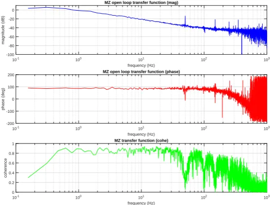
To control the MZ, one of the two mirrors is placed on a piezoelectric ceramic. Acting on the piezo, the difference path length can be actively modified. The error signal is provided by a photodiode that samples the MZ reflected signal (i.e. the beam used as pump for the OPO). The optimal working point to the control loop is when the MZ reflection is linear with the steepest slope, that is,RoptM Z=RmeanM Z . A scheme of the control loop is in Fig.4.5. The measurements of the MZ transfer function and the MZ open loop transfer function are presented in Fig.4.6 and Fig.4.7 respectively.
E
inE
TE
RFigure 4.5: Scheme of the MZ control loop. The beam reflected by the second beam splitter of the MZ interferometer is sampled by a beam splitter (with 700ppm reflectivity and diverted to a (in loop) photodiode: the difference of the developed signal with respect to a reference signal is used to control the MZ arm length difference. For the measurements of Fig.4.8, the beam transmitted by the sampling beam splitter was collected by a (out of loop) photodiode.
frequency (Hz) 101
102
103
104
magnitude (dB)
-60 -40 -20 0
MZ transfer function (mag)
frequency (Hz)
101 102 103 104
coherence
0 0.2 0.4 0.6 0.8
1 MZ transfer function (cohe) frequency (Hz) 101
102
103
104
phase (deg)
-800 -600 -400 -200 0
200 MZ transfer function (phase)
4.1. SQUEEZED VACUUM SOURCE OPTICAL LAYOUT 39
frequency (Hz) 10-1
100
101
102
103
magnitude (dB)
-100 -80 -60 -40 -20 0
MZ open loop transfer function (mag)
frequency (Hz) 10-1
100
101
102
103
coherence
0 0.2 0.4 0.6 0.8
1 MZ transfer function (cohe) frequency (Hz) 10-1
100
101
102
103
phase (deg)
-200 -100 0 100
200 MZ open loop transfer function (phase)
Figure 4.7: Measurement of the MZ open loop transfer function. The unitary gain frequency is approximately 1 Hz and the servo is a standard PI.
to reach the target power stability.
4.1.2
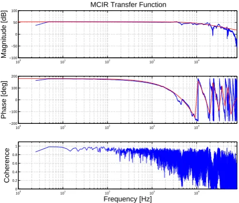
Infrared mode-cleaner (MCIR)
The infrared mode cleaner (MCIR) is one of the two traveling wave cavities present on the optical bench. This resonator is used as an optical low pass filter for high frequency phase noise, moreover it provides mode spatial filtering on the incoming beam and it also works as a polarization filter. This cavity is placed along the homodyne local oscillator beam path, as close as possible to the homodyne detector. As illustrated in Fig.4.9 (left), this resonator is set up as a three mirror Fabry-Perot ring cavity. Fig.4.9 (right) shows a picture of the IR mode cleaner mounted on the optical bench. The input and output cavity mirror are two identical plano-plano polished mirror with power transmittivityTp= 1.25% for p polarized light andTs= 700ppm for s polarized light
both at an incidence angleθi= 45◦±2◦. The third cavity mirror is a polished, curved mirror with
a radius of curvature of 1 m and a transmittivity of T = 300ppm for both light polarizations. The round trip length is 545 mm. The two plano-plano mirror are mechanically attached to a monolithic invar3 spacer and the curved mirror is mechanically attached to a piezoelectric ceramic, in turn attached to the same invar spacer. This design was adopted to guarantee high mechanical stability and low length fluctuation due to thermal variation. The computed waist size is 389.4µm in the transverse or horizontal plane and 389.6µm in the sagittal or vertical plane with respect to the plane identified by the cavity path. The cavity finesse Fs,p can be
3Invar, also known generically as FeNi36, is a nickeliron alloy notable for its low coefficient of thermal expansion
time (sec) #105
0 0.5 1 1.5 2 2.5
Voltage (V)
-0.263 -0.262 -0.261 -0.26 -0.259 -0.258 -0.257 -0.256
-0.255 out of loop tranmission
-0.263 -0.262 -0.261 -0.26 -0.259 -0.258 -0.257 -0.256 -0.255
counts 0 2000 4000 6000 time (sec) #105
0 0.5 1 1.5 2 2.5
Voltage (V)
-2.513 -2.512 -2.511 -2.51 -2.509 -2.508
-2.507 in loop transmission
-2.513 -2.512 -2.511 -2.51 -2.509 -2.508 -2.507
counts 0 1000 2000 3000
Figure 4.8: Measurement of the green power stability over two days.
Figure 4.9: (left) Schematic of the IR mode cleaner; in red the optical path of the IR light inside the mode cleaner. (right) Picture of the IR mode cleaner mounted on the optical bench inside the cleanroom at Virgo site.
computed, for s and p polarization respectively, via
Fs,p=
π(R1R22s,p)1/4
1−q1−R1R22s,p
(4.1.2)
where R1 is the power reflectivity of the curved mirror andR2s,p are the power reflectivity of
the plano-plano mirrors for the s and p polarization respectively.
In our case, eq(4.1.2) givesFs≈3700 for s polarized light andFp≈247 for p polarized light.
4.1. SQUEEZED VACUUM SOURCE OPTICAL LAYOUT 41
149 kHz for s polarization and 2.23 MHz for p polarization.
-80 -40 0 40 80
0,00 0,02 0,04 0,06
-80 -40 0 40 80
-0,8 -0,6 -0,4 -0,2 0,0 0,2 T ra n s mis s ion [ V ]
νFWHM= 165.21kHz
E rr o r S ig n a l [V ] Frequency [MHz] errsign slope = 7.66 V/MHz
Figure 4.10: Cavity scan near the s pol TEM00. The top line shows the cavity transmission, while the bottom one is the error signal obtained by demodulating at 80 MHz the cavity reflection sig-nal. The transmission peak has been fitted and the FWHM is reported (νF W HM = 165.21 kHz).
The linear part of the error signal has been also fitted to calibrate the error signal.
Fig.4.10 shows a cavity scan of the s pol TEM00. The fitted cavity linewidth is slightly higher than expected. This results in a finesse for s polarization ofFs= 3330. The finesse for p
polarization was also measured, giving Fp = 205. Also in this case the finesse is slightly lower
than expected.
The infrared mode cleaner is held on resonance to the main laser field using a standard PDH technique. The laser light is phase modulated by an EOM with a frequency of 80 MHz by the same EOM which provides the modulation for the SHG cavity. The cavity reflection signal is acquired by a photodetector and analogically demodulated. The bottom trace of Fig.4.10 shows the demodulated signal obtained withphase one electronics.
Fig.4.11 shows the cavity scan of the p pol TEM00 demodulated reflection, that is the p pol error signal used to lock the cavity length. The orange curve is the fit of the data performed using equations of [37]. The fit is in good agreement with the experimental data.
Fig.4.12 shows the cavity transfer function of the infrared mode cleaner with phase one
electronics. On this cavity thephase two electronics was tested. In particular the transmission and reflections photodetectors have been upgraded and we migrated the control loop from the commercial PXI system to the SAT group board (see Section 4.2.2).
Fig.4.13 shows the cavity transfer function of the infrared mode cleaner with phase two
frequency (Hz) ×108
-1.5 -1 -0.5 0 0.5 1 1.5
Vo