www.geosci-model-dev.net/5/649/2012/ doi:10.5194/gmd-5-649-2012
© Author(s) 2012. CC Attribution 3.0 License.
Geoscientific
Model Development
The CSIRO Mk3L climate system model version 1.0 – Part 2:
Response to external forcings
S. J. Phipps1,2,3,4, L. D. Rotstayn5, H. B. Gordon5, J. L. Roberts2,3,6, A. C. Hirst5, and W. F. Budd1,2,3 1Institute of Antarctic and Southern Ocean Studies, University of Tasmania, Australia
2Antarctic Climate & Ecosystems CRC, Hobart, Tasmania, Australia
3Tasmanian Partnership for Advanced Computing, Hobart, Tasmania, Australia 4Climate Change Research Centre, University of New South Wales, Australia
5Centre for Australian Weather and Climate Research: A partnership between CSIRO and the Bureau of Meteorology,
Aspendale, Victoria, Australia
6Australian Antarctic Division, Kingston, Tasmania, Australia
Correspondence to: S. J. Phipps ([email protected])
Received: 14 November 2011 – Published in Geosci. Model Dev. Discuss.: 7 December 2011 Revised: 12 April 2012 – Accepted: 24 April 2012 – Published: 14 May 2012
Abstract. The CSIRO Mk3L climate system model is a coupled general circulation model, designed primarily for millennial-scale climate simulation and palaeoclimate re-search. Mk3L includes components which describe the at-mosphere, ocean, sea ice and land surface, and combines computational efficiency with a stable and realistic control climatology. It is freely available to the research community. This paper evaluates the response of the model to external forcings which correspond to past and future changes in the climate system.
A simulation of the mid-Holocene climate is performed, in which changes in the seasonal and meridional distribu-tion of incoming solar radiadistribu-tion are imposed. Mk3L cor-rectly simulates increased summer temperatures at northern mid-latitudes and cooling in the tropics. However, it is un-able to capture some of the regional-scale features of the mid-Holocene climate, with the precipitation over North-ern Africa being deficient. The model simulates a reduc-tion of between 7 and 15 % in the amplitude of El Ni˜no-Southern Oscillation, a smaller decrease than that implied by the palaeoclimate record. However, the realism of the simu-lated ENSO is limited by the model’s relatively coarse spatial resolution.
Transient simulations of the late Holocene climate are then performed. The evolving distribution of insolation is im-posed, and an acceleration technique is applied and assessed. The model successfully captures the temperature changes in
each hemisphere and the upward trend in ENSO variability. However, the lack of a dynamic vegetation scheme does not allow it to simulate an abrupt desertification of the Sahara.
To assess the response of Mk3L to other forcings, transient simulations of the last millennium are performed. Changes in solar irradiance, atmospheric greenhouse gas concentra-tions and volcanic emissions are applied to the model. The model is again broadly successful at simulating larger-scale changes in the climate system. Both the magnitude and the spatial pattern of the simulated 20th century warming are consistent with observations. However, the model underes-timates the magnitude of the relative warmth associated with the Mediaeval Climate Anomaly.
Finally, three transient simulations are performed, in which the atmospheric CO2 concentration is stabilised at
two, three and four times the pre-industrial value. All three simulations exhibit ongoing surface warming, reduced sea ice cover, and a reduction in the rate of North Atlantic Deep Water formation followed by its gradual recovery. Antarc-tic Bottom Water formation ceases, with the shutdown being permanent for a trebling and quadrupling of the CO2
concen-tration. The transient and equilibrium climate sensitivities of the model are determined. The short-term transient response to a doubling of the CO2concentration at 1 % per year is a
1 Introduction
The CSIRO Mk3L climate system model is a computationally-efficient atmosphere-land-sea ice-ocean general circulation model, designed for the study of cli-mate variability and change on millennial timescales. It incorporates a spectral atmospheric general circulation model, a z-coordinate ocean general circulation model, a dynamic-thermodynamic sea ice model and a land surface scheme with static vegetation. The zonal and meridional resolutions used by all components are 5.625◦and∼3.18◦, respectively, with 18 vertical levels in the atmosphere and 21 vertical levels in the ocean. Flux adjustments are applied to improve the realism of the simulated control climate and to minimise drift. Mk3L represents a new version of the CSIRO climate model, the history of which is described by Smith (2007). The atmosphere, land and sea ice mod-els are reduced-resolution versions of those used by the CSIRO Mk3 coupled model (Gordon et al., 2002), while the ocean model is taken from the CSIRO Mk2 coupled model (Gordon and O’Farrell, 1997). A 1000-yr climate simulation can be completed in around 45 days on a typical state-of-the-art (Intel Core 2 Duo) desktop computer, with greater throughput being possible on high-performance computing facilities. Mk3L is freely available to the research community, and access to the Subversion repository can be obtained by completing the online application form at http://www.tpac.org.au/main/csiromk3l/.
Part 1 of this paper (Phipps et al., 2011) describes the model physics and software, analyses the control climatol-ogy, and evaluates the ability of the model to simulate the modern climate. The simulated states of the atmosphere, cryosphere and ocean are found to be in broad agreement with observations. However, biases on the regional scale in-clude excessive cloud cover and precipitation in the tropics, deficient winter sea ice cover in the Northern Hemisphere, and a deep ocean which is too cold and too fresh. Mk3L pro-duces reasonable representations of the leading modes of in-ternal climate variability in both the tropics and extratropics. However, the simulated El Ni˜no-Southern Oscillation is too weak, too slow and characterised by excessive modulation on interdecadal timescales.
This paper describes and evaluates the response of ver-sion 1.0 of Mk3L to external forcings which correspond to past and future changes in the climate system. A variety of simulations are performed and the response of the model is compared, as appropriate, with observations, proxy-based re-constructions of past climate and with the response of other models. Section 2 evaluates the ability of Mk3L to simu-late the climate of the mid-Holocene. Section 3 then anal-yses the transient response of the model to the changing sea-sonal and meridional distribution of insolation during the late Holocene. Section 4 presents a transient simulation of the last millennium, and evaluates the response of Mk3L to changes in solar irradiance, greenhouse gas concentrations and
vol-canic emissions. Finally, Sect. 5 explores the transient and equilibrium responses of the model to scenarios in which the atmospheric CO2concentration is stabilised at two, three and
four times the pre-industrial level.
The aim of this paper is to characterise the response of Mk3L to external forcings and to identify possible deficien-cies in the model physics. As such, the focus is upon describ-ing the response of the model, rather than upon conductdescrib-ing detailed analyses of each experiment. Many of the simula-tions presented herein justify more extensive scientific anal-ysis, which will form the basis of future manuscripts.
2 The climate of the mid-Holocene
2.1 Introduction
The climate of the mid-Holocene (6000 yr Before Present, where the present is defined as the year 1950 CE) has fre-quently been used to evaluate the ability of climate mod-els to simulate climatic change (e.g. Joussaume et al., 1999; Masson et al., 1999; Braconnot et al., 2000; Bonfils et al., 2004; Braconnot et al., 2007a,b). This epoch represents the relatively recent past, and extensive and high-quality recon-structions of the mid-Holocene climate are available against which to evaluate the performance of the models (Yu and Harrison, 1996; Cheddadi et al., 1997; Hoelzmann et al., 1998; Jolly et al., 1998a,b; Prentice and Webb, 1998; Kohfeld and Harrison, 2000; Prentice et al., 2000; Brewer et al., 2007; Bartlein et al., 2011). The external forcing, which is mainly due to changes in the seasonal and meridional distribution of insolation arising from changes in the Earth’s orbital parame-ters, is also well-known and can be precisely defined (Berger, 1978; Braconnot et al., 2007a). Changes in sea level and the extent of land ice relative to the present day are sufficiently small that they can be neglected.
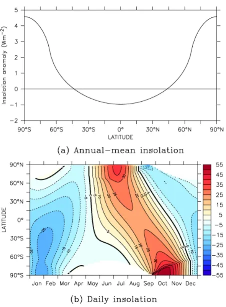
During the mid-Holocene, the Earth’s axial tilt was slightly greater than it is today (24.105◦at 6000 yr BP, as op-posed to the present-day value of 23.446◦). This gave rise to a slight change in the meridional distribution of annual-mean insolation, with a reduction of∼1 W m−2in the tropics and an increase of∼4.5 W m−2at the poles (Fig. 1a). How-ever, as a result of the precession of the equinoxes, there were much larger differences in the seasonal cycle (Fig. 1b). Inso-lation was considerably greater than today during the North-ern Hemisphere summer and SouthNorth-ern Hemisphere spring, and considerably reduced during the Southern Hemisphere summer.
Fig. 1. The insolation (W m−2) at 6000 yr BP, expressed as an anomaly relative to the present day: (a) the annual mean, and (b) daily values.
and plant macrofossils indicate that it was extensively vege-tated (Jolly et al., 1998a,b; Joussaume et al., 1999; Bartlein et al., 2011).
Many studies have used climate models to simulate the climate of the mid-Holocene, often motivated by a desire to evaluate the performance of the models. In particular, the Paleoclimate Modelling Intercomparison Project (PMIP) has used the climate of the mid-Holocene as a basis to systemati-cally compare the performance of different models. PMIP1 used stand-alone atmospheric general circulation models forced by present-day sea surface temperatures (Harrison et al., 1998; Joussaume et al., 1999; Masson et al., 1999; Bra-connot et al., 2000; Bonfils et al., 2004; Hoar et al., 2004), while PMIP2 has employed coupled atmosphere-ocean gen-eral circulation models (Braconnot et al., 2007a,b). The mod-els are successful at capturing both an intensification and northward migration of the African monsoon; however, they are unable to capture the magnitude of the northward shift (Braconnot et al., 2007a,b).
The failure to adequately capture the changes in the African monsoon can be attributed, at least in part, to the static nature of the vegetation and land surface types within these simulations. The vegetation is unable to respond fully to the changed atmospheric conditions, and the extent of
vegetation feedbacks cannot therefore be simulated. Early studies which incorporated dynamic vegetation models into atmosphere-ocean general circulation models confirmed the role of both oceanic and vegetation feedbacks in giving rise to the wetter conditions that prevailed over Northern Africa during the mid-Holocene (Braconnot et al., 1999; Levis et al., 2004). While further confirming the role of the vegetation feedback, PMIP2 found that the magnitude of the feedback was smaller than in previous studies, possibly because of an inconsistency in the experimental design (Braconnot et al., 2007a,b). Changes in surface albedo have also been shown to be important (Vamborg et al., 2011). Thus the mid-Holocene African monsoon remains a daunting test of the ability of models to simulate climatic change.
In addition to changes in the mean state of the cli-mate, changes in the nature of climate variability dur-ing the mid-Holocene have also received attention. Proxy records indicate a strengthening of interannual variability in the tropical Pacific Ocean during the Holocene. For example, analysis of corals from Papua New Guinea re-veals that El Ni˜no-Southern Oscillation (ENSO) activity at ∼6500 yr BP was much weaker than at present (Tudhope et al., 2001). A 15 000-yr sedimentation record from an alpine lake in Ecuador indicates a lack of variability on El Ni˜no timescales prior to 7000 yr BP, with ENSO-type vari-ability beginning at ∼7000 yr BP and reaching its modern strength at ∼5000 yr BP (Rodbell et al., 1999). A further analysis of a 12 000-yr sedimentation record from the same lake confirms the initiation of ENSO at∼7000 yr BP, with strong variability on millennial timescales thereafter (Moy et al., 2002). Pollen evidence from Northern Australia also indicates a strengthening of ENSO during the Holocene, with the onset of an ENSO-dominated climate at ∼4000 yr BP (Shulmeister and Lees, 1998).
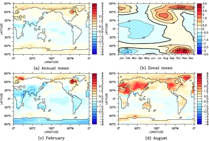
Fig. 2. The average surface air temperature (K) for years 201–1200 of experiment 6KA, expressed as an anomaly relative to CONTROL: (a) the annual mean, (b) the zonal mean, (c) February, and (d) August. In (a), (c) and (d), only values that are significant at the 95% confidence level are shown.
2.2 Experimental design
The ability of Mk3L to simulate the climate of the mid-Holocene is evaluated in this section. The model was inte-grated under mid-Holocene boundary conditions, following the protocol specified by PMIP2 (http://pmip2.lsce.ipsl.fr/) and PMIP3 (http://pmip3.lsce.ipsl.fr/). Relative to the pre-industrial control simulation (Part 1; Phipps et al., 2011), the Earth’s orbital parameters were changed to values ap-propriate for 6000 yr BP. The atmospheric CO2concentration
was also reduced from 280 ppm to 277 ppm, in order to im-pose a radiative forcing equivalent to the specified reduction in the atmospheric CH4concentration from 760 to 650 ppb.
This was necessary as the radiation scheme in version 1.0 of Mk3L does not directly account for the radiative effects of anthropogenic greenhouse gases other than CO2.
The model was initialised from the state of the control sim-ulation at the end of model year 100. The first 100 yr of the mid-Holocene simulation are excluded from analysis to al-low the model to respond to the change in external forcing. This was sufficient for it to reach equilibrium, with global-mean surface air temperature (SAT) and sea surface tempera-ture (SST) changing by less than 0.01 K between the first and second centuries of the simulation. The following analysis is therefore based on model years 201 to 1200. The control and
mid-Holocene simulations shall be referred to hereafter as CONTROL and 6KA, respectively. Over the 1000-yr analy-sis period, global-mean SAT changes by−0.08 K in CON-TROL and +0.02 K in 6KA. The results presented here are not corrected for drift.
2.3 Surface air temperature
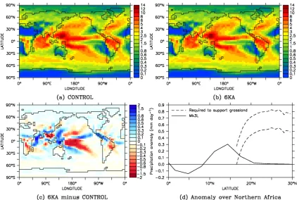
Fig. 3. The annual-mean precipitation (mm day−1) for years 201–1200 of experiments CONTROL and 6KA: (a) CONTROL, (b) 6KA, (c) 6KA minus CONTROL, and (d) the zonal-mean difference over Northern Africa (20◦W–30◦E). In (c), only values that are significant at the 95 % confidence level are shown. In (d), minimum and maximum estimates of the precipitation increase required to support grassland at each latitude are also shown (Joussaume et al., 1999).
temperature at high latitudes; for example, there is no cooling over the Southern Ocean in response to the negative insola-tion anomalies between December and July.
The strongest warming at northern mid-latitudes occurs in August. SAT is higher across the Northern Hemisphere land-masses, with summer warming of up to 5.0 K over Greenland and up to 4.3 K over Eurasia (Fig. 2d). As a result of the sea-sonal nature of the insolation anomalies and the large thermal inertia of the ocean, the warming over the ocean is modest. The average SAT increase across the Northern Hemisphere for the period June–September is 0.55 K; this is consistent with the PMIP2 models, which exhibit temperature increases of between 0.35 and 0.8 K (Braconnot et al., 2007a).
In contrast, cooling occurs at low latitudes and through-out the Sthrough-outhern Hemisphere in February (Fig. 2c). SAT is reduced by up to 2.7 K over land in the tropics, and by up to 2.2 K over Antarctica. The average SAT change across the Northern Hemisphere for the period December–February is−0.15 K; this is also consistent with the PMIP2 models, which exhibit temperature changes ranging from approxi-mately−0.9 to+0.1 K (Braconnot et al., 2007a).
2.4 Precipitation
The annual-mean precipitation for experiments CONTROL and 6KA, respectively, is shown in Fig. 3a and b, while Fig. 3c shows the difference between the two simulations. The intensification and northward migration of the African-Asian monsoon is reflected in the annual-mean precipitation, with increased precipitation over Northern Africa and South-east Asia.
The changes in the African monsoon are apparent from Fig. 3d, which shows the change in the zonal-mean precip-itation over Northern Africa. Also shown are the minimum and maximum estimates of the increase in precipitation, rel-ative to the present day, that would be required in order to support grassland at each latitude (Joussaume et al., 1999). Biome reconstructions indicate that grasslands were present at least as far north as 23◦N during the mid-Holocene (Jolly
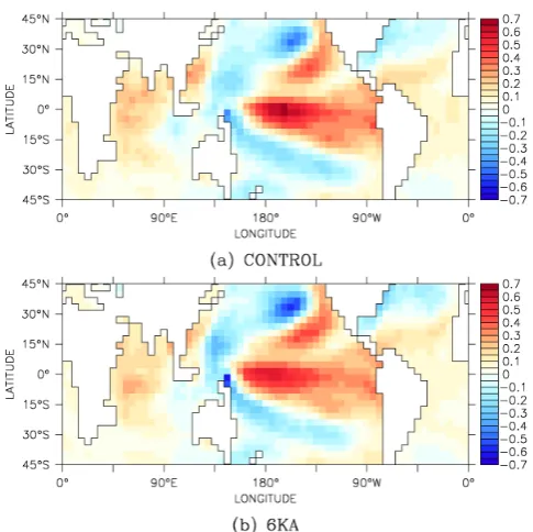
Fig. 4. The leading principal component (K) of the monthly sea surface temperature anomalies in the region 45◦S–45◦N for years 201–1200 of experiments CONTROL and 6KA: (a) CONTROL, and (b) 6KA.
greater than∼17◦N. The majority of models which partici-pated in PMIP2 also fail to simulate sufficient precipitation over Northern Africa (Braconnot et al., 2007a). The reasons for this deficiency are unclear, with vegetation feedbacks found to increase the simulated precipitation in only one of the three models which were integrated both with and with-out dynamic vegetation schemes. One possibility is that the models do not include schemes which represent the radia-tive effects of dust; studies using models which incorporate dust schemes have shown that this is an important control on Northern African precipitation (Yoshioka et al., 2007).
The magnitudes of the changes in the African-Asian mon-soon, as simulated by Mk3L, are consistent with the PMIP2 models. For the period June–September, the simulated pcipitation over Northern Africa (defined here as the re-gion 20◦W–30◦E, 10–25◦N) increases by 0.35 mm day−1 or 28 % relative to CONTROL; this is consistent with the PMIP2 models, which exhibit increases relative to the pre-industrial control simulations ranging from 0.2 to 1.6 mm day−1and from 5 to 140 %. For North India (defined
here as the region 70–100◦E, 20–40◦N), the simulated
pre-cipitation increases by 0.69 mm day−1or 22 %; again, this is
consistent with the PMIP2 models, which exhibit increases ranging from 0.2 to 0.8 mm day−1and from 5 to 33 % (Bra-connot et al., 2007a).
Table 1. El Ni˜no-Southern Oscillation statistics for years 201–1200 of experiments CONTROL and 6KA: The standard deviation (K) of the monthly sea surface temperature anomaly in the Ni˜no 3 (150–90◦W, 5◦S–5◦N), Ni˜no 3.4 (170–120◦W, 5◦S–5◦N) and Ni˜no 4 (160◦E–150◦W, 5◦S–5◦N) regions; the maximum temper-ature anomaly (K) associated with the leading principal component (PC1) of monthly sea surface temperature anomalies in the region 45◦S–45◦N; and the percentage change (6KA minus CONTROL).
Control 6KA % change
Ni˜no 3 0.395 0.367 −7 Ni˜no 3.4 0.513 0.453 −12 Ni˜no 4 0.501 0.520 +4
PC1 0.673 0.572 −15
2.5 El Ni ˜no-Southern Oscillation
The leading principal component of the monthly SST anoma-lies within the region 45◦S–45◦N, for experiments CON-TROL and 6KA, is shown in Fig. 4. El Ni˜no-Southern Os-cillation (ENSO; Philander, 1990) is the leading mode of variability in tropical SSTs for both experiments. However, in 6KA, the principal components are shifted slightly to the west. The largest positive anomalies occur at 163◦W in the case of CONTROL, whereas they occur at 180◦E in the case of experiment 6KA. This shift causes the maximum variability to lie outside the Ni˜no 3.4 region, with the re-sult that the principal component more closely resembles the observed present-day interdecadal variability in the Pacific Ocean (Zhang et al., 1997; Lohmann and Latif, 2005).
Fig. 5. The equatorial zonal wind stress (N m−2) and sea surface temperature (SST,◦C) for years 201–1200 of experiment 6KA: (a) monthly-mean zonal wind stress, expressed as anomalies relative to CONTROL, (b) monthly-monthly-mean sea surface temperature, expressed as anomalies relative to CONTROL, (c) annual-mean zonal wind stress, and (d) annual-mean sea surface temperature. The values shown are averages over the region 5◦S–5◦N.
The simulated changes in the zonal wind stress and SST over the equatorial Pacific Ocean are shown in Fig. 5. Con-sistent with the hypothesis of Zheng et al. (2008), the creased insolation during the boreal summer leads to an in-crease in the strength of the easterly trade winds during the boreal summer and autumn (Fig. 5a). This gives rise to an in-crease in the zonal temperature gradient (Fig. 5d), and acts to suppress the development of El Ni˜no events. The magnitudes of the zonal wind stress and SST changes are similar to those simulated by Liu et al. (2000).
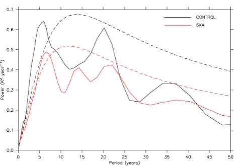
The wavelet power spectra of the simulated Ni˜no 3.4 SST anomalies, for experiments CONTROL and 6KA, are shown in Fig. 6. Wavelet spectra were calculated using the method of Torrence and Compo (1998), modified following Liu et al. (2007) to ensure a physically consistent definition of energy. As reflected in the reduced variability in the Ni˜no 3 and Ni˜no 3.4 regions, experiment 6KA exhibits less power at al-most all timescales. There is also an increase in the period of the simulated ENSO, with peak variability occurring at 6.6 yr in 6KA as opposed to 6.0 yr in CONTROL.
2.6 Summary
Mk3L is capable of simulating the larger-scale differences between the climate of the mid-Holocene and that of the present day, with warmer summers at northern mid-latitudes and slight cooling in the tropics. However, discrepancies arise on the regional scale, with the model being unable to capture the full extent of the estimated precipitation changes over Northern Africa. The incorporation of a dynamic veg-etation scheme and/or a dust scheme into Mk3L might im-prove its ability to simulate such changes.
The model simulates a reduction in the strength of El Ni˜no-Southern Oscillation, accompanied by a westward shift in the location of greatest variability. The simulated reduction in the strength of ENSO is smaller in magnitude than that implied by the palaeoclimate record. This discrepancy may reflect deficiencies in the representation of ENSO within the model, with the simulated present-day ENSO being too weak and too slow relative to observations (Part 1; Phipps et al., 2011). These deficiencies are likely to be a consequence of the model’s reduced spatial resolution.
Flux adjustments are applied in Mk3L, both to improve the realism of the simulated control climate and to minimise drift. Studies using two other climate system models have shown that flux-adjusted and non-flux-adjusted versions of the same model can exhibit differences in the response to mid-Holocene boundary conditions. Brown et al. (2008) find that the large-scale changes in temperature and precipitation are similar between two different versions of HadCM3, and therefore that flux adjustments have no leading-order impact. However, there are regional-scale differences in the response of the model, particularly in the tropical Pacific. Kitoh et al. (2007) analyse two different versions of MRI-CGCM2.3, and reach a similar conclusion. However, flux adjustments are found to influence the simulated response of ENSO to ex-ternal forcings in both models. In the flux-adjusted versions, the changes in ENSO amplitude in response to mid-Holocene boundary conditions are +4 % and −2 % in HadCM3 and MRI-CGCM2.3, respectively. In contrast, in the non-flux-adjusted versions, the ENSO amplitude changes by−14 % and−15 %, respectively. These differences in the response of each model are attributed to the effect of flux adjust-ments on seasonal phase-locking (Brown et al., 2008) and on the strength of the ocean-atmosphere feedback (Kitoh et al., 2007). A comparison with proxy data therefore sug-gests that the non-flux-adjusted versions of HadCM3 and MRI-CGCM2.3 are more realistic, as they simulate stronger reductions in ENSO variability. However, as the flux adjust-ments act via their effects on the control climate, there is no evidence that they directly affect the response of either model. Notable biases exist in the control climates of both non-flux-adjusted models, and it is therefore hard to argue that these versions are more realistic overall (Brown et al., 2008; Kitoh et al., 2007).
3 Transient simulations of the late Holocene
3.1 Introduction
In recent years, the computational power of high-performance computing facilities has increased to the point where it is now possible to use fully-coupled atmosphere-ocean general circulation models (AOGCMs) such as Mk3L to carry out multi-millennial simulations. This has enabled the use of AOGCMs to explore the transient evolution of the climate system over periods such as the late Holocene (Lorenz and Lohmann, 2004; Liu et al., 2006; Lorenz et al., 2006; Schurgers et al., 2006; Fischer and Jungclaus, 2011; Varma et al., 2012). The computational expense of a state-of-the-art AOGCM can be sufficiently prohibitive that it is necessary to reduce the execution time, and some of these studies have therefore employed the acceleration technique of Lorenz and Lohmann (2004). This technique accelerates the rate of change in the Earth’s orbital parameters, on the assumption that the response timescale of the climate system is much shorter than the timescales on which orbital forcing is significant.
This section examines the transient response of Mk3L to the insolation changes that arose during the late Holocene from the pseudo-cyclical variations in the Earth’s orbital pa-rameters. Using the mid-Holocene simulation from Sect. 2 as the initial state, the model is used to conduct transient simu-lations of the period from 6000 yr BP to the present day.
3.2 Experimental design
Three transient simulations were conducted for the pe-riod from 6000 yr BP to the present day (0 yr BP, equiva-lent to 1950 CE). The acceleration technique of Lorenz and Lohmann (2004) was employed, with acceleration factors of 5, 10 and 20. These experiments are designated HOLO5, HOLO10 and HOLO20, and have total durations of 1200, 600 and 300 model years, respectively.
Each experiment was initialised from the state of experi-ment 6KA at the end of model year 1000. The Earth’s orbital parameters were then varied, with the appropriate accelera-tion factors being applied. As the intenaccelera-tion of these experi-ments is to study the response of the model to orbital forcing, all the other boundary conditions were held constant, with a solar constant of 1365 W m−2and an atmospheric CO2
con-centration of 277 ppm. Although this is 3 ppm lower than the concentration of 280 ppm used in the control simulation, this equates to a radiative forcing of only 0.06 W m−2. Apart
from the orbital parameters and this difference in the atmo-spheric CO2 concentration, the boundary conditions were
otherwise identical to the control.
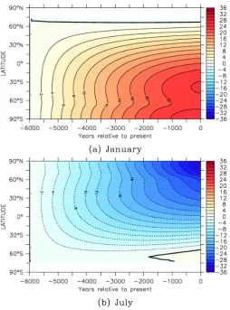
Fig. 7. The evolution of monthly-mean insolation (W m−2) during the late Holocene, expressed as an anomaly relative to 6000 yr BP: (a) January, and (b) July.
shows the evolution of the mean January and July insola-tion during the late Holocene as a funcinsola-tion of latitude, and shows that the trends at most latitudes are monotonic. The forcing applied to the model can therefore be characterised as consisting of decreasing insolation during the Northern Hemisphere summer and Southern Hemisphere spring, with increasing insolation during the Southern Hemisphere sum-mer.
3.3 Surface air temperature
The evolution of the simulated mean SAT during the North-ern and SouthNorth-ern Hemisphere summers is shown in Fig. 8. Starting from the relatively warm mid-Holocene state, the Northern Hemisphere cools steadily in response to the de-creasing insolation. Likewise, the Southern Hemisphere, starting from the relatively cool mid-Holocene state, warms steadily in response to the increasing insolation. In both hemispheres, the mean temperatures stabilise during the fi-nal millennium as the rates of change in insolation decrease. Any differences between the three experiments are consistent with the amplitude of the simulated internal variability. This
Fig. 8. The evolution of hemispheric-mean surface air temperature during experiments HOLO5 (red), HOLO10 (green) and HOLO20 (blue): (a) Northern Hemisphere, August, and (b) Southern Hemi-sphere, February. The values shown are running means across five model years.
demonstrates that the assumption underlying the acceleration technique is valid, at least in these circumstances. Neither is there any evidence from Fig. 8 that model drift accounts for any divergence between the experiments. Because of the use of accelerated boundary conditions, none of the experiments span more than 1200 model years; the acceleration technique therefore acts to reduce the contribution of any background model drift towards the simulated long-term trends.
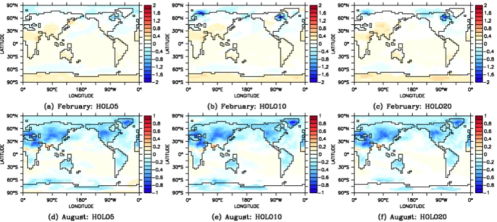
Fig. 9. The linear trend in surface air temperature (K per 1000 yr) during the late Holocene: (a–c) February, experiments HOLO5, HOLO10 and HOLO20, respectively, and (d–f) August, experiments HOLO5, HOLO10 and HOLO20, respectively. Only values that are significant at the 95 % confidence level are shown. Note the different scale bars for the February and August plots.
Over most of the Earth’s surface, the trends are indepen-dent of the magnitude of the acceleration factor used. How-ever, as the acceleration factor is increased, there are fewer values that are significant at the 95 % confidence level. Over sea ice in the winter hemisphere, there are also locations where the magnitude of the trend differs between experi-ments; this is most apparent over the Barents Sea and Hud-son Bay in February. With the sea ice cover acting to insulate the atmospheric boundary layer from the underlying ocean, the magnitude of the interannual variability in SAT is large compared to the long-term trend. As the acceleration factor is increased, the trend therefore becomes increasingly poorly constrained. Lorenz and Lohmann (2004), who use a larger range of acceleration factors (10 and 100), also find that the SAT trends in some regions can depend upon the factor. The mismatches in their case are attributed to a combination of stochastic variability and model drift.
3.4 Precipitation
The evolution of the June–September precipitation over Northern Africa (20◦W–30◦E, 10–25◦N) during each ex-periment is shown in Fig. 10a, with the total precipitation exhibiting a slow and steady decline towards the present-day value. As with the surface air temperature, any diffences be-tween the three experiments are consistent with the ampli-tude of the simulated internal variability.
The gradual drying trend exhibited by the model contrasts with the abrupt desertification of Northern Africa that ap-pears to have occurred in reality. Terrigenous marine sedi-ments indicate that the Sahara underwent a transition from a vegetated state to an arid state over a period of several decades to centuries, centred at 5490±190 yr BP (deMeno-cal et al., 2000); however, the spatial extent and duration of these changes is still under discussion (Kr¨opelin et al., 2008; Brovkin and Claussen, 2008). Mk3L includes a land sur-face scheme with static vegetation, and the model is there-fore incapable of simulating such a transition. The lack of dynamic vegetation means that the model omits an impor-tant feedback within the climate system and, as discussed in Sect. 2, it is possible that this accounts for the deficiency in the simulated mid-Holocene precipitation over Northern Africa. Rather, Mk3L simulates a physically-driven precipi-tation trend that might have occurred in the absence of vege-tation feedbacks. This is consistent with transient simulations conducted using models with dynamic vegetation schemes, which show an ongoing precipitation decline even after the Sahara has transitioned to an arid state (deMenocal et al., 2000; Liu et al., 2006).
The linear trends in annual-mean precipitation, derived by calculating the line of best fit at each gridpoint, are shown in Fig. 10b–d. As with SAT, the spatial variations in the trends reflect the precipitation anomalies, relative to the present day, that existed at the start of the simulation period (Fig. 3c). Negative trends over Northern Africa, India and southeast
Asia reflect the weakening and southward migration of the African-Asian monsoon system. There is also a southward migration of the South American monsoon and an eastward migration of the monsoonal precipitation associated with the South Pacific Convergence Zone. The spatial patterns of the trends exhibited by the three experiments are in good agree-ment, indicating the robustness of the acceleration technique. However, as with SAT, increases in the acceleration factor cause a reduction in the area over which the trends are sig-nificant at the 95 % confidence level.
3.5 Ocean temperature
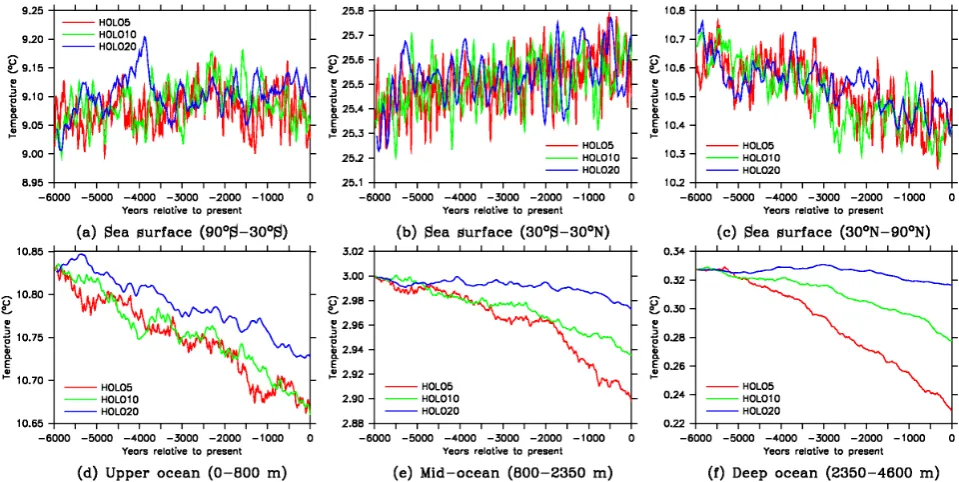
Figure 11a–c shows the evolution of the simulated annual-mean SST in the southern extratropics (90–30◦S), the trop-ics (30◦S–30◦N) and the northern extratropics (30–90◦N).
Starting from a time when annual-mean insolation in the tropics was lower than today (Fig. 1a), tropical SSTs warm steadily as insolation increases (Fig. 11b). In contrast, start-ing from a time when annual-mean insolation at high lat-itudes was higher than today, SSTs in the northern extra-tropics cool steadily as insolation decreases (Fig. 11c). No equivalent cooling signal is seen in the southern extratrop-ics (Fig. 11a), as the Southern Ocean spans the mid-latitudes where the change in annual-mean insolation is small. Any differences between the three experiments are consistent with the amplitude of the simulated internal variability, indicat-ing that the assumption underlyindicat-ing the acceleration technique is valid, at least for the surface ocean. However, the use of acceleration does cause interdecadal variability within each simulation to manifest itself as centennial- to millennial-scale variations; this is most apparent in the southern extrat-ropics.
The evolution of the mean potential temperature for the upper ocean (0–800 m), mid-ocean (800–2350 m) and deep ocean (2350–4600 m) is shown in Fig. 11d–f. A cooling trend is apparent at all depths, which is driven by the reduction in SSTs at high northern latitudes and hence a reduction in the temperature of North Atlantic Deep Water (not shown). However, the responses of the three experiments differ. In the upper ocean, experiments HOLO5 and HOLO10 exhibit con-sistent trends, but the simulated rate of cooling is slower in HOLO20. The divergence between the three experiments be-comes greater with depth; in the deep ocean, the cooling sim-ulated by experiment HOLO5 is almost completely absent in HOLO20. The assumption underlying the acceleration tech-nique – namely, that the response timescale of the climate system is negligibly short compared to the timescales on which orbital forcing is significant – therefore breaks down when considering changes in the ocean interior.
Fig. 11. The evolution of annual-mean potential temperature during experiments HOLO5 (red), HOLO10 (green) and HOLO20 (blue): (a) the sea surface (90–30◦S), (b) the sea surface (30◦S–30◦N), (c) the sea surface (30–90◦N), (d) the upper ocean (0–800 m), (e) the mid-ocean (800–2350 m), and (f) the deep ocean (2350–4600 m). The values shown are running means across five model years.
being simulated, such as glacial cycles, then it is likely that the use of large acceleration factors would give rise to signifi-cant errors in the simulated ocean temperatures. These might influence the density structure of the ocean to such an extent as to have a significant impact upon the thermohaline circu-lation, with consequences for the accuracy of the simulated climate at the Earth’s surface. Nonetheless, there is no evi-dence of any such errors arising for the acceleration factors and time periods considered here.
3.6 El Ni ˜no-Southern Oscillation
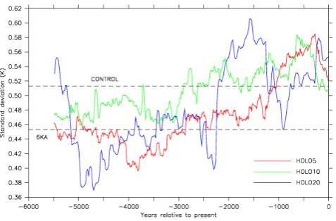
The evolution of ENSO variability during each experi-ment, as measured by the standard deviation in the monthly Ni˜no 3.4 SST anomaly, is shown in Fig. 12. A moving win-dow with a width of 1000 calendar years is used to deter-mine the standard deviation; this is equivalent to 200, 100 and 50 model years, respectively, for experiments HOLO5, HOLO10 and HOLO20. To allow the variability to be sam-pled right up to the present day, each experiment was inte-grated for a further 500 calendar years.
An overall upward trend in ENSO variability is simulated by experiment HOLO5, which is consistent with the sup-pressed variability, relative to the present day, at the start of the simulation period. Considerable millennial-scale vari-ability is also apparent, with a period of relatively weak ENSO variability centred at around 3800 yr BP, and a period of stronger-than-present ENSO variability centred at around 300 yr BP. Strong millennial-scale variability is also
encoun-tered in proxy-based reconstructions such as that of Moy et al. (2002), although the use of an acceleration technique here prevents any direct comparison between the model and reconstructions.
Experiments HOLO10 and HOLO20 simulate an overall upward trend in ENSO variability over the late Holocene, as for HOLO5. However, there are considerable differences between the three experiments. In particular, the natures of the simulated millennial-scale variations differ, and the am-plitude of the millennial-scale variability is larger in experi-ment HOLO20 than in the others. The sampling interval cor-responds to just 50 model years for the latter experiment. This lack of robustness displayed by the results is consistent with the model-based analysis of Wittenberg (2009), which concludes that at least 500 yr of data may be required in or-der to adequately sample ENSO variability. While this is a formidable requirement from an observational perspective, the use of large ensembles can allow for adequate sampling of ENSO variability within model simulations.
3.7 Summary
lack of a dynamic vegetation scheme prevents the model from simulating the abrupt desertification that appears to have occurred in reality. There is also a gradual increase in ENSO variability.
The acceleration technique of Lorenz and Lohmann (2004) was used to reduce the duration of each experiment. Trends in hemispheric-mean surface air temperature, and in precipitation over Northern Africa, are found to be indepen-dent of the acceleration factor used. This is consistent with the underlying assumption that orbital forcing operates on timescales much longer than the response timescale of the climate system. However, the use of acceleration reduces the sampling frequency such that there is insufficient data to ade-quately constrain trends in surface air temperature or precipi-tation at locations with large interannual variability, or to ad-equately sample changes in ENSO variability on millennial timescales. This is due to the acceleration technique, and is not a shortcoming of the model itself. The use of acceleration also influences the simulated temperatures in the ocean inte-rior, which might introduce significant errors if large accel-eration factors were to be used to simulate very long periods of time.
4 Transient simulation of the last millennium
4.1 Introduction
The last millennium provides a valuable opportunity to eval-uate climate system models and to study the sensitivity of the climate system. Proxy-based reconstructions are avail-able that have both high temporal resolution and widespread geographical coverage (e.g., Mann et al., 2009). The bound-ary conditions on the climate system over this period, in-cluding atmospheric trace gases, solar irradiance and vol-canic emissions, are also reasonably well constrained (e.g., Schmidt et al., 2011). The sensitivity of the climate system to different forcings can therefore be studied, and climate sys-tem models can be evaluated by forcing them with the known boundary conditions and then comparing the resulting simu-lations against the available proxy data. For these reasons, recent studies have used a range of climate system models to study the climate of the last millennium (Fan et al., 2009; Liu et al., 2009; Jungclaus et al., 2010; Servonnat et al., 2010; Hofer et al., 2011).
In this section, the transient response of Mk3L to known climatic forcings during the period 1001 to 2000 CE is stud-ied. Specifically, the model is forced with changes in the Earth’s orbital parameters, solar irradiance, anthropogenic greenhouse gases and stratospheric sulphate aerosols aris-ing from volcanic emissions. The resultaris-ing simulation is then compared against observations and proxy-based reconstruc-tions of past climate.
Fig. 12. The evolution of the standard deviation of the monthly sea surface temperature anomaly in the Ni˜no 3.4 region (170–120◦W, 5◦S–5◦N) during experiments HOLO5 (red), HOLO10 (green) and HOLO20 (blue). A moving window with a width of 1000 calendar years is used to calculate the standard deviation. Horizontal dashed lines show the amplitude of ENSO variability in experiments CON-TROL and 6KA.
4.2 Experimental design
The Earth’s orbital parameters are calculated internally by the model, using the method of Berger (1978). However, the insolation changes arising from orbital forcing over the last millennium are relatively modest (Fig. 13a). At low latitudes, the changes consist of increasing insolation during the first half of the year, accompanied by decreasing insolation dur-ing the second half. At high latitudes, relatively strong de-creases in insolation occur during the Northern Hemisphere summer and autumn, as well as during the Southern Hemi-sphere spring and summer. These decreases are accompanied by smaller increases in insolation during the other times of the year.
Fig. 13. The boundary conditions applied during experiment LAST1000: (a) the change in insolation arising from orbital forcing, 2000 CE minus 1001 CE (W m−2), (b) total solar irradiance, (c) effective total solar irradiance, taking into account stratospheric sulphate aerosols arising from volcanic eruptions, and (d) equivalent atmospheric carbon dioxide concentration.
is only ∼0.9 W m−2 below the mean value for the 1986–
1996 CE solar cycle, as opposed to estimates of∼3.2 and ∼2.8 W m−2for Lean et al. (1995) and Lean (2000),
respec-tively.
The values for stratospheric sulphate aerosol loading were taken from the Ice-core Volcanic Index 2 (IVI2; Gao et al., 2008). Following the documentation supplied with the dataset, the 1982 El Chich´on eruption was incorporated by adding a loading of 14 Tg to the Northern Hemisphere timeseries. Version 1.0 of Mk3L does not include a sul-phate aerosol scheme, and so the values for the stratospheric sulphate aerosol loading were converted into an equivalent anomaly in the TSI. This process involved three distinct stages, as follows. Stage 1: following Stothers (1984) and Gao et al. (2008), the global aerosol loading was divided by 150 Tg to obtain a global-mean value for the aerosol opti-cal depth (which is a dimensionless quantity). To allow for the effects of coagulation, the loadings were scaled accord-ing to a two-thirds power law for values greater than 15 Tg (Crowley, 2000). Stage 2: following Wigley et al. (2005) and Gao et al. (2008), the aerosol optical depth was multiplied by −20 W m−2 to obtain a global-mean radiative forcing. Stage 3: to obtain an equivalent anomaly in the TSI, the radia-tive forcing was multiplied by a factor of 5.69; this represents the ratio between the TSI (1365 W m−2) and the observed net downward shortwave flux at the top of the atmosphere (240 W m−2).
The volcanic anomalies were added to the timeseries of TSI derived from Steinhilber et al. (2009) to derive val-ues of an effective TSI. The resulting timeseries is shown in Fig. 13c, and it is these values that were used to force the model. The largest volcanic eruption to take place dur-ing the last millennium is that of 1258 CE, the location of which is unknown (Gao et al., 2008). This gives rise to a radiative forcing of −13 W m−2, equivalent to a 5.5 % re-duction in TSI. Other eruptions which give rise to a reduc-tion of at least 2.5 % in TSI are Kuwae (1452 CE), Laki (1783 CE) and Tambora (1815 CE). The radiative forcing caused by the 1991 CE Pinatubo eruption is −3.2 W m−2, equivalent to a 1.3 % reduction in TSI and in agree-ment with both observationally-derived values of −2.7± 1.0 W m−2 (Minnis et al., 1993) and calculated values of around−3 W m−2(Forster et al., 2007). Limitations in both
the model physics and the reconstruction result in inherently unrealistic representations of volcanic eruptions. The radia-tive forcing associated with each eruption is both spatially and seasonally uniform, being applied from 1 January to 31 December of the year in which the eruption took place. However, the annual- and global-scale representation of the impacts should be at least approximately correct.
Fig. 14. The changes in surface temperature over the last millennium according to the “all proxy” timeseries of Mann et al. (2009) (black) and experiment LAST1000 (annual values in red, 10-yr running mean in green): (a) Northern Hemisphere surface air temperature, and (b) Ni˜no 3 sea surface temperature. The values shown are expressed as anomalies relative to the 1001–1850 CE mean. The 95 % confidence interval for Mann et al. (2009) is indicated by grey shading.
the climate system can therefore be more important than so-lar forcing on a global scale. Volcanic forcing is strongest in the 13th century, with an average radiative forcing of −0.34 W m−2, and weakest in the 11th, 14th and 16th
cen-turies, with an average radiative forcing of −0.08 W m−2. These figures compare with a peak radiative forcing asso-ciated with the Maunder Minimum of −0.16 W m−2, but are still small in magnitude compared with present-day an-thropogenic radiative forcing of around+1.6 W m−2(Forster et al., 2007). However, volcanic eruptions and changes in TSI affect the climate system in ways that cannot be represented by a simple radiative forcing (Shindell et al., 2003). Strato-spheric sulphate aerosols and solar ultraviolet irradiance both affect atmospheric ozone concentrations and the thermal structure of the atmosphere. Without an aerosol scheme or an atmospheric chemistry scheme, version 1.0 of Mk3L can-not simulate these effects.
Anthropogenic greenhouse gas concentrations were taken from MacFarling Meure et al. (2006). This dataset combines the ice core record from Law Dome in Antarctica with di-rect measurements taken at Cape Grim in Tasmania, Aus-tralia. The concentrations of CO2, CH4 and N2O are
pro-vided, with a 20-yr smoother having been applied in the case of CO2and CH4, and a 40-yr smoother having been applied
in the case of N2O. These concentrations were converted into
equivalent CO2concentrations (COe2), which were calculated
so as to impose a radiative forcing equivalent to that
aris-ing from the changes in the concentrations of each of the three gases. The expressions provided in Table 6.2 of Ra-maswamy et al. (2001) were used, with the unperturbed CH4
and N2O concentrations set to 760 and 270 ppb, respectively.
The resulting timeseries of COe2values is shown in Fig. 13d, and it is these values that were used to force the model. Prior to 1800 CE, COe2 varies within the narrow range 269 to 282 ppm, before rising to 410 ppm by 2000 CE. Relative to the CO2 concentration of 280 ppm used in the control
simulation, these values equate to a radiative forcing of be-tween−0.22 and+0.04 W m−2prior to 1800 CE, increasing to+2.04 W m−2by 2000 CE. Because version 1.0 of Mk3L does not include an aerosol scheme, anthropogenic aerosols were not considered here. However, given a suitable recon-struction of the radiative forcing arising from past changes in anthropogenic aerosols, it would be possible to take these into account via adjustments to the equivalent CO2
concen-tration.
2011). The Law Dome dataset of MacFarling Meure et al. (2006) is used here to provide the concentrations of all an-thropogenic greenhouse gases, whereas the dataset supplied by CMIP5/PMIP3 uses data from multiple ice cores to derive the N2O concentration (Schmidt et al., 2011). Both these
dif-ferences in the experimental design are negligible.
To conduct a transient simulation of the last millennium, Mk3L was first initialised from the state of the control simu-lation at the end of model year 100. It was then integrated for 100 yr under static 1000 CE boundary conditions, with this being a sufficient duration for the model to respond to the small change in boundary conditions relative to the control simulation. Finally, the transient simulation was initialised from the state of the model at the end of the 1000 CE snap-shot simulation. This transient simulation shall be referred to hereafter as LAST1000. Over the 1000-yr period of the con-trol simulation which corresponds to experiment LAST1000, drift in global-mean SAT amounts to a cooling of just 0.08 K. The results presented here are not corrected for drift.
4.3 The response of the model
The simulated changes in Northern Hemisphere (NH) SAT and the mean SST in the Ni˜no 3 region (150–90◦W, 5◦S– 5◦N) are shown in Fig. 14. They are compared with the re-construction of Mann et al. (2009), hereafter referred to as M2009, which is derived from a global multiproxy network comprising more than a thousand individual records. Tem-perature is reconstructed by calibrating the proxy network against instrumental data covering the period from 1850 to 1995 CE. Proxy data with both annual and decadal resolu-tion are used to derive the reconstrucresolu-tion, so only variaresolu-tions on interdecadal timescales are meaningful. Both the simu-lated and reconstructed temperatures are expressed in Fig. 14 as anomalies relative to the 1001–1850 CE mean, and the±2 standard deviation uncertainty range is shown for M2009.
During the pre-industrial period, Mk3L captures the decadal-to-centennial scale variations in NH SAT well. Prior to 1850 CE, the ten-year running mean for the model rarely exceeds the confidence interval for M2009. However, the model underestimates the magnitude of the relative warmth during the 11th century, being∼0.2 K cooler than the recon-struction. It also simulates a strong cooling in response to the volcanic eruption of 1258 CE. This is not apparent in M2009, although the decadal resolution of the reconstruction would result in a greatly attenuated signal. Prior to 1850 CE, there is no long-term trend in the simulated Ni˜no 3 SST. This is con-sistent with the long-term trend in M2009 over the bulk of this period, except for the failure to capture the relatively cool conditions during the 11th century. Mk3L therefore fails to simulate the La Ni˜na-like conditions that appear to have pre-vailed during the Mediaeval Climate Anomaly (Mann et al., 2009).
During the industrial period, the model slightly overesti-mates the warming trend in NH SAT relative to the
recon-struction, with the simulated mean temperature anomaly for 1991–2000 CE being∼0.2 K warmer than M2009. This may reflect the fact that the model simulation does not account for the effects of anthropogenic aerosols. However, as the model correctly simulates the observed global-mean warming dur-ing the 20th century (Sect. 4.5), it may also indicate that the reconstruction underestimates the magnitude of the anthro-pogenic warming trend. Nonetheless, the simulated increase in the Ni˜no 3 SST over the industrial period is consistent with the reconstruction.
The response of the model will now be analysed in more detail, with the sensitivities to natural and anthropogenic forcings considered separately.
4.4 Sensitivity to natural forcings
On annual and decadal timescales, volcanic forcing gener-ally exceeds in magnitude the variations in total solar irra-diance (TSI). Only on centennial timescales is it therefore possible to determine the sensitivity of the model to changes in solar output. The situation is complicated by the fact that, of the four solar grand minima to have occurred during the last millennium, three have coincided with the three largest volcanic eruptions: the eruption of 1258 CE occurred shortly before the Wolf Minimum, the Kuwae eruption (1452 CE) occurred during the Sp¨orer Minimum, and the Tambora erup-tion (1815 CE) occurred during the Dalton Minimum. Only the Maunder Minimum (∼1645–1715 CE) was free of major volcanic eruptions.
According to M2009, the NH SAT during the period 1645–1715 CE differs from the 1001–1850 CE mean by a statistically-significant margin only during the first three years (1645–1647 CE). This appears to be in response to the Mount Parker volcanic eruption in 1641 CE, which causes the NH SAT to dip∼0.4 K below the 1001–1850 CE mean. For the remainder of the Maunder Minimum, it is not possi-ble to reject the null hypothesis that the temperature was the same as the 1001–1850 CE mean.
Mk3L simulates an average NH SAT during the Maunder Minimum that is 0.12 K below the 1001–1850 CE mean, with a 95 % confidence interval of±0.03 K. Despite the lack of major volcanic eruptions, the coldest 71-yr period during ex-periment LAST1000 is 1641–1711 CE, which coincides al-most exactly with the Maunder Minimum. Furthermore, the period 1641–1711 CE is 0.05±0.04 K colder than the 71-yr period that precedes it and 0.10±0.04 K colder than the 71-yr period that follows it. This strongly suggests that the simulated cooling during this period is a response to solar forcing, and that the sensitivity of the model to the reduction in solar output associated with the Maunder Minimum is a hemispheric-mean cooling of∼0.05–0.1 K.
in NH SAT of ∼1.1 K. There is considerable evidence of widespread climatic, social and economic disruptions in the aftermath of this eruption (Stothers, 2000), accompanied by a reduction of 1.5 K in summer temperatures in the Euro-pean Alps (B¨untgen et al., 2006). However, no hemisphere-wide temperature signal is apparent in M2009. There are a number of possible explanations for this discrepancy: the decadal resolution of the reconstruction; the fact that proxy networks which incorporate tree ring data underestimate the magnitude of the cooling in response to large volcanic erup-tions (Robock, 2005); or the fact that the climatic response to volcanic eruptions is neither spatially nor seasonally uni-form (Robock, 2000). This latter issue might cause proxy networks to exhibit differing sensitivities to individual erup-tions. It would also mean that the parameterisation of vol-canic eruptions as a uniform radiative forcing, as in experi-ment LAST1000, is highly unrealistic on both a regional and seasonal scale. Alternatively, Timmreck et al. (2009) show that once the size distributions of aerosol particles are taken into account in an Earth system model, the magnitude of the simulated temperature response to the 1258 CE eruption can be reduced substantially. This challenges the simple relation-ship assumed here between stratospheric sulphate aerosol loading and aerosol optical depth, and suggests that the scal-ing applied to loadscal-ings greater than 15 Tg (Sect. 4.2) does not adequately reflect the increase in particle size arising from coagulation.
In contrast, M2009 records decadal-scale cooling in re-sponse to the Kuwae (1452 CE) and Tambora (1815 CE) eruptions. The decadal-scale response of Mk3L is consis-tent with the reconstruction in both cases. During the three years following the 1991 CE Pinatubo eruption, which be-gins on 1 January 1991 CE in experiment LAST1000, the model simulates a NH SAT that remains at least 0.2 K be-low the 1990 CE value. The three-year period 1991–1993 CE is 0.28±0.09 K cooler than the preceding three-year pe-riod 1988–1990 CE. This is consistent with the analysis of Thompson et al. (2009) who, after removing other influences on global-mean SAT, find a peak cooling of∼0.4 K one year after the eruption, with cooling of at least∼0.2 K persisting for three years.
Figure 15 shows the simulated temperature anomalies dur-ing the Mediaeval Climate Anomaly (MCA; 1001–1250 CE) and the Little Ice Age (LIA; 1400–1700 CE). These periods represent the pre-industrial extremes in the centennial-scale NH SAT over the last millennium, and thus they provide a test of the ability of the model to simulate centennial-scale changes in the climate. Although Mann et al. (2009) define the MCA as beginning in 950 CE, the year 1001 CE is used here as this is the first year of experiment LAST1000; regard-less, Mann et al. (2009) note that the temperature patterns as-sociated with the MCA and LIA are not sensitive to the pre-cise time intervals used. Relative to the 1001–1850 CE mean, the model simulates weak warming during the MCA and weak cooling during the LIA. These changes are amplified
Fig. 15. The simulated changes in surface air temperature (K) dur-ing the Mediaeval Climate Anomaly (MCA; 1001–1250 CE) and the Little Ice Age (LIA; 1400–1700 CE), according to experiment LAST1000: (a) the MCA minus the 1001–1850 CE mean, (b) the LIA minus the 1001–1850 CE mean, and (c) the MCA minus the LIA.
over Central Asia and at high latitudes, particularly over the Southern Ocean. However, apart from some regional cool-ing over the North Atlantic durcool-ing the MCA, the changes are otherwise relatively uniform. The model therefore appears to simulate a primarily thermal response to the forcing changes, with the lack of spatial variations indicating little in the way of a dynamical response.
cooling, particularly that associated with the La Ni˜na-like pattern of temperature changes over the Pacific Basin. How-ever, neither the GISS-ER nor the NCAR CSM 1.4 mod-els capture this signature either, suggesting that it may be stochastic in origin (Mann et al., 2009).
4.5 Sensitivity to anthropogenic forcings
Mk3L simulates an increase in global-mean SAT between 1861–1900 CE and 1991–2000 CE of 0.62±0.06 K, which is consistent with the observationally-based estimate of 0.6± 0.2 K (Folland et al., 2001). Over the 20th century, the tran-sient sensitivity of the model to increasing concentrations of anthropogenic greenhouse gases is therefore consistent with observations. However, the model simulation does not ac-count for the effects of anthropogenic aerosols, which act to cool the climate system (Forster et al., 2007). This may indicate that the transient climate sensitivity of Mk3L is too low. The simulated global-mean SAT for the period 1991– 2000 CE is 14.08±0.05◦C, which is 0.46 K warmer than the pre-industrial control simulation (Part 1; Phipps et al., 2011) but still 0.33 K cooler than the mean value of 14.41◦C ac-cording to the NCEP-DOE Reanalysis 2 (Kanamitsu et al., 2002, hereafter referred to as NCEP2).
The spatial pattern of the 20th century warming is shown in Fig. 16a and is consistent with observed trends (Folland et al., 2001). Warming occurs over most of the Earth’s sur-face, and is strongest at high latitudes and over Central Asia. However, there is also some localised cooling; this is partic-ularly strong in the North Atlantic Ocean, where the cooling signal arises within the model because of a weakening of the meridional overturning circulation (Fig. 17). North Atlantic Deep Water formation decreases in response to elevated an-thropogenic greenhouse gas concentrations during the indus-trial period, with the mean rate for the period 1951–2000 CE (12.8 Sv) being 14 % weaker than the mean rate for the pe-riod 1001–1850 CE (14.9 Sv).
The discrepancy in the average SAT for 1991–2000 CE, relative to NCEP2, is shown in Fig. 16b. Relative to the pre-industrial control simulation (Fig. 4 of Part 1; Phipps et al., 2011), the warming at high latitudes and cooling over Hud-son Bay leads to a slightly improved agreement with the re-analysis. The root-mean-square error in annual-mean SAT relative to NCEP2 is 1.77 K, as opposed to an error of 1.90 K for the pre-industrial control.
During the 20th century, the model simulates a warming trend throughout the troposphere, accompanied by a cool-ing trend throughout the stratosphere (Fig. 16c). The magni-tude of these trends is consistent with observations, which indicate cooling of the stratosphere between 1958 CE and 2004 CE of∼1.5 K, accompanied by a warming of the tro-posphere of up to 0.5 K (Trenberth et al., 2007). The dis-crepancy in the average zonal-mean temperature for 1991– 2000 CE, relative to NCEP2, is shown in Fig. 16d. The sim-ulated 20th century changes improve the agreement with
the reanalysis, relative to the pre-industrial control simula-tion (Fig. 7 of Part 1; Phipps et al., 2011). In particular, the stratospheric cooling reduces the magnitude of the positive anomalies in the lower stratosphere.
4.6 Summary
Mk3L is broadly successful at capturing the observed changes in the climate system over the last millennium. The response to solar and volcanic forcing during the pre-industrial period is largely consistent with the reconstruc-tion of Mann et al. (2009), with the model simulating a hemispheric-mean cooling of∼0.05–0.1 K in response to the reduction in solar output associated with the Maunder Min-imum. However, the model simulates strong cooling in re-sponse to the volcanic eruption of 1258 CE, which does not appear in the reconstruction. The model also underestimates the magnitude of the relative warmth associated with the Me-diaeval Climate Anomaly, and fails to reproduce the La Ni˜na-like signature in the temperature changes. This suggests that it may be failing to capture the dynamical response of the climate system to the natural radiative forcings that appear to have given rise to the MCA (Mann et al., 2009).
The simulated response to increasing concentrations of anthropogenic greenhouse gases is consistent with observa-tions, with the model simulating warming of 0.62±0.06 K during the 20th century. However, as the effects of anthro-pogenic aerosols are not taken into account, this suggests that the transient climate sensitivity of the model may be too low. The warming trend extends throughout the troposphere, ac-companied by a stronger cooling trend in the stratosphere.
The incorporation of schemes for aerosols and atmo-spheric chemistry would allow the effects of solar and vol-canic forcing to be better represented within Mk3L; in particular, the model would be able to take into account the size distributions of aerosol particles and would be able to simulate the effects of ozone photochemistry. Such enhance-ments would also allow the model to represent the effects of anthropogenic aerosols. Rotstayn et al. (2007), for example, used a version of the CSIRO model similar to Mk3L but in-cluding an interactive aerosol scheme. They found that their model was successful at reproducing the observed decadal changes in global-mean SAT over the period 1871–2000 CE, including the mid-20th century cooling.
5 CO2stabilisation experiments
5.1 Introduction
In this section, the transient and equilibrium responses of Mk3L to an increase in the atmospheric carbon dioxide con-centration are investigated. Scenarios are employed in which the CO2concentration is increased at 1 % per year, before
Fig. 16. The changes in atmospheric temperature (K) over the 20th century according to experiment LAST1000: (a) surface air tempera-ture, 1991–2000 CE average minus 1861–1900 CE average, (b) average surface air temperature for 1991–2000 CE, Mk3L minus NCEP2, (c) zonal-mean temperature, 1991–2000 CE average minus 1861–1900 CE average, and (d) average zonal-mean temperature for 1991– 2000 CE, Mk3L minus NCEP2.
Fig. 17. The change in the rate of North Atlantic Deep Water formation during experiment LAST1000. The values shown are five-year running means.
with the models which participated in the Coupled Model Intercomparison Project (CMIP; Meehl et al., 2000, 2007a).
A number of studies have assessed the response of ver-sions of the CSIRO model to increases in atmospheric car-bon dioxide. Using slab ocean versions of the CSIRO Mk1 and Mk2 general circulation models, Watterson et al. (1999) found climate sensitivities, defined as the equilibrium global-mean SAT increase in response to a doubling of the CO2
con-centration, of 4.84 and 4.34 K, respectively. A subsequent
study assessed the slab ocean version of the CSIRO Mk3.0 general circulation model, and found that weaker feedbacks gave it a lower climate sensitivity of 3.08 K (Watterson and Dix, 2005). Another version of the CSIRO model, similar in nature to Mk3L, was found to have a climate sensitivity of 3.52 K when coupled to a mixed-layer ocean model (Rot-stayn and Penner, 2001).
Fig. 18. The atmospheric carbon dioxide concentration applied dur-ing experiments CONTROL (black), 2CO2 (red), 3CO2 (green) and 4CO2 (blue). Vertical dashed lines indicate model years 100, 170, 211 and 240.
studied. Hirst (1999) investigated both the transient and the long-term responses of the model to a trebling of the CO2
concentration. Bi et al. (2001, 2002) and Bi (2002) expanded upon this work, using the acceleration technique of Bryan (1984) to integrate the model to equilibrium. The final re-sponse to a CO2 trebling was found to be an increase in
global-mean SAT of 7.3 K.
The long-term responses of other AOGCMs to increased atmospheric CO2 concentrations have also been studied
(Manabe and Stouffer, 1993, 1994; Stouffer and Manabe, 1999, 2003; Senior and Mitchell, 2000; Voss and Mikola-jewicz, 2001; Bryan et al., 2006; Danabasoglu and Gent, 2009). In combination with the CMIP models, these simula-tions provide a basis against which to compare the response of Mk3L.
5.2 Experimental design
Three transient climate change simulations are presented. They were initialised from the state of the control simulation at the end of model year 100. The atmospheric carbon diox-ide concentration was then increased at 1 % per year from the start of model year 101, until it reached either two, three or four times the pre-industrial value of 280 ppm (experiments 2CO2, 3CO2 and 4CO2, respectively). The final CO2
con-centrations of 560, 840 and 1120 ppm were reached in model years 170, 211 and 240, respectively, and the concentration was held constant thereafter (Fig. 18). Each experiment was then integrated until the end of model year 4000.
Previous sections have compared the response of Mk3L with observations and palaeoclimate reconstructions, and have sought to identify deficiencies in the model physics. Such an approach is not possible for simulations of future climate states, whether realistic or idealised, and this section
is therefore restricted to a comparison of the transient and equilibrium responses of Mk3L with those of other models.
5.3 Surface air temperature
The evolution of the simulated global-mean SAT during each experiment is shown in Fig. 19a. The global-mean SAT in-creases rapidly as the CO2 concentration is increased, and
continues to increase once the CO2 concentration has been
stabilised. However, the rate of change decreases over time as the simulations progress towards thermal equilibrium. The slow cooling trend exhibited by the control simulation, as discussed in Part 1 (Phipps et al., 2011), is apparent.
Prior to model year 170, the CO2concentrations for each
of the three transient experiments are identical; each experi-ment therefore exhibits the same temperature increases. Dur-ing the transient stage of experiment 4CO2, the global-mean SAT warms by 1.6 K upon a doubling of the CO2
concentra-tion, and by 3.7 K upon a quadrupling. The ongoing warming exhibited by experiments 2CO2, 3CO2 and 4CO2 indicates that they have not reached thermal equilibrium, even by the end of a 4000-yr simulation. By the final century of exper-iment 2CO2, global-mean SAT has increased by 3.9 K rela-tive to the first century of the control simulation and is still increasing at a rate of 0.015 K century−1.
The transient climate response (TCR) of a climate model is defined as the global-mean SAT anomaly for the period 61–80 yr after the CO2concentration begins to increase (e.g.
Gregory and Forster, 2008). The value obtained here for Mk3L, and the 95% confidence interval, is 1.59 K±0.08 K. This value lies within the 5–95 % uncertainty range of 1.2– 2.4 K for the AOGCMs which were analysed by the IPCC Fourth Assessment Report (AR4), but is slightly less than the mean value of 1.76 K (Meehl et al., 2007b). It is also consis-tent with the estimated 5–95 % uncertainty range for the true climate system of 1.3–2.3 K (Gregory and Forster, 2008). A low value for the TCR is consistent with the fact that the model correctly simulates the magnitude of the 20th century warming trend, despite not being forced with changes in an-thropogenic aerosols (Sect. 4.5). Given that anan-thropogenic aerosols act to cool the climate system (Forster et al., 2007), the model might be expected to over-estimate the 20th cen-tury warming trend if its TCR was the same as that of the true climate system.
The equilibrium climate sensitivity (ECS) of a climate model is defined as the equilibrium increase in global-mean SAT in response to a doubling of the CO2 concentration.
Fig. 19. The changes in annual-mean surface air temperature and sea ice extent during experiments CONTROL (black), 2CO2 (red), 3CO2 (green) and 4CO2 (blue): (a) the global-mean surface air temperature, (b) the Northern Hemisphere sea ice extent, and (c) the Southern Hemisphere sea ice extent. The values shown are five-year running means. Vertical dashed lines indicate model years 100, 170, 211 and 240. Note the change in the scale of the time axis at year 500.
the end of experiment 2CO2. Values of the ECS between 3.85 and 4.41 K are consistent with the 5–95 % uncertainty range for the AR4 AOGCMs of 2.1–4.4 K, but are greater than the mean value of 3.26 K (Meehl et al., 2007b). They are also consistent with the “likely” range for the true climate system of 2–4.5 K (Meehl et al., 2007b).
It should be emphasised that there is a difference in methodology between this study and AR4. As a result of the computational expense of state-of-the-art AOGCMs, the ECS is typically determined by replacing the oceanic compo-nent of a model with a non-dynamic slab ocean (e.g. Meehl et al., 2007b). In contrast, the full Mk3L AOGCM is studied here. Although flux adjustments are used, the thermohaline circulation – and therefore the ocean heat transport – is free to evolve, unlike in a slab ocean model. Danabasoglu and Gent (2009) show that the slab ocean approach
underesti-mates the ECS by just 0.14 K in the case of CCSM3, but no attempt appears to have been made to validate this approach across multiple models. Earlier studies that addressed this question using other models were unable to reach definitive conclusions, either because the simulations were too short or because of drift in the control simulation (Stouffer and Man-abe, 1999; Senior and Mitchell, 2000; Gregory et al., 2004). Prior to Danabasoglu and Gent (2009), only one study ap-pears to have been successful in determining the ECS of an AOGCM other than the CSIRO model by integrating it to equilibrium: Stouffer and Manabe (2003) determine an ECS for the GFDL model of 4.33 K.