Vol. 5, No. 2, 2013 Article ID IJIM-00295, 12 pages Research Article
An application of fuzzy logic in measuring a systems effectiveness
M. Gr. Voskoglou ∗ †
————————————————————————————————–
Abstract
In the present paper we use principles of fuzzy logic to develop a general model representing several processes in a systems operation characterized by a degree of vagueness and/or uncertainty. We also introduce three alternative measures of a fuzzy systems effectiveness connected to our general model. These measures include the systems total possibilistic uncertainty, the Shannons entropy properly modified for use in a fuzzy environment and the centroid method in which the coordinates of the center of mass of the graph of the membership function involved provide an alternative measure of the systems performance. The advantages and disadvantages of the above measures are discussed and a combined use of them is suggested for achieving a worthy of credit mathematical analysis of the corresponding situation. Finally, an application of is presented for the Problem Solving process illustrating the use of our results in practice.
Keywords: Systems theory; Fuzzy sets and logic; Possibility; Uncertainty theory; Problem solving.
—————————————————————————————————–
1
Introduction: Systems’
mod-elling and fuzzy logic
A
system is a set of interacting or interde-pendent components forming an integrated whole. A system comprises multiple views such as planning, analysis, design, implementation, de-ployment, structure, behavior, input and output data, etc. As an interdisciplinary and multi- per-spective domain systems theory brings together principles and concepts from ontology, philoso-phy of science, information and computer sci-ence, mathematics, as well as physics, biology, engineering, social and cognitive sciences, man-agement and economics, strategic thinking, fuzzi-ness and uncertainty, etc. Thus, it serves as a bridge for an interdisciplinary dialogue between autonomous areas of study. The emphasis with∗Corresponding author. [email protected]
†School of Technological Applications, Graduate Tech-nological Educational Institute of Patras, Greece.
systems theory shifts from parts to the organiza-tion of parts, recognizing that interacorganiza-tions of the parts are not static and constant, but dynamic processes.
Most systems share common characteristics in-cluding structure, behavior, interconnectivity (the various parts of a system have functional and structural relations to each other), sets of functions, etc. We scope a system by defining its boundary; this means choosing which entities are inside the system and which are outside of it, part of the environment.
The systems modelling is a basic principle in engi-neering, in natural and in social sciences. When we face a problem concerning a systems opera-tion (e.g. maximizing the productivity of an in-dustry, minimizing the functional costs of a com-pany, etc) a model is required to describe and represent the systems multiple views. The model is a simplified representation of the basic charac-teristics of the real system including only its en-tities and features under concern. In this sense,
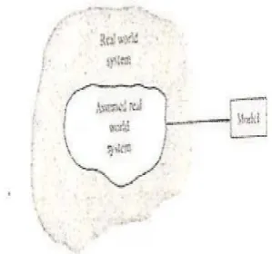
no model of a complex system could include all features and/or all entities belonging to the sys-tem. In fact, in this way the models structure could become very complicated and therefore its use in practice could be very difficult and some-times impossible. Therefore the construction of the model usually involves a deep abstracting pro-cess on identifying the systems dominant vari-ables and the relationships governing them. The resulting structure of this action is known as the assumed real system (see Figure 1). The model, being an abstraction of the assumed real system, identifies and simplifies the relationships among these variables in a form amenable to analysis. A
Figure 1: A graphical representation of the modelling process.
system can be viewed as a bounded transforma-tion, i.e. as a process or a collection of processes that transforms inputs into outputs with the very broad meaning of the concept. For example, an output of a passengers bus is the movement of people from departure to destination.
Many of these processes are frequently character-ized by a degree of vagueness and/or uncertainty. For example, during the processes of learning, of reasoning, of problem-solving, of modelling, etc, the human cognition utilizes in general concepts that are inherently graded and therefore fuzzy. On the other hand, from the teachers point of view there usually exists an uncertainty about the degree of students success in each of the stages of the corresponding didactic situation.
There used to be a tradition in science and en-gineering of turning to probability theory when one is faced with a problem in which uncertainty plays a significant role. This transition was justi-fied when there were no alternative tools for
deal-ing with the uncertainty. Today this is no longer the case. Fuzzy logic, which is based on fuzzy sets theory introduced by Zadeh [28] in 1965, provides a rich and meaningful addition to standard logic. The applications which may be generated from or adapted to fuzzy logic are wide-ranging and provide the opportunity for modelling under con-ditions which are inherently imprecisely defined, despite the concerns of classical logicians. Many systems may be modelled, simulated and even replicated with the help of fuzzy logic, not the least of which is human reasoning itself (e.g. [21], [24], [26], [27], etc). A real test of the effectiveness of an approach to uncertainty is the capability to solve problems which involve different facets of uncertainty. Fuzzy logic has a much higher prob-lem solving capability than the standard proba-bility theory. Most importantly, it opens the door to construction of mathematical solutions of com-putational problems which are stated in a natural language. In contrast, standard probability the-ory does not have this capability, a fact which is one of its principal limitations.
All these gave us the impulsion to introduce prin-ciples of fuzzy logic to describe in a more effective way a systems operation in situations character-ized by a degree of vagueness and/or uncertainty. For general facts on fuzzy sets and logic and on uncertainty theory we refer freely to the book of Klir and Folger [4].
2
The general fuzzy model
U ={a, b, c, d, e}.
We are going to attach to each stage Si a fuzzy subset, Ai of U. For this, if nia, nib, nic, nid and nie denote the number of entities that faced very low, low, intermediate, high and very high suc-cess at stageSi respectively,i= 1,2,3, we define the membership functionmAifor eachx inU, as follows:
mA(x) =
1, 4n
5 < nix ≤n,
0.75, 3n
5 < nix≤ 4n
5 ,
0.5, 2n
5 < nix ≤ 3n
5 ,
0.25, n
5 < nix ≤ 2n
5 , 0, 0< nix≤
Then the fuzzy subset Ai of U corresponding to Si has the form: In order to represent all possi-ble profiles (overall states) of the systems entities during the corresponding process we consider a fuzzy relation, say R, in U3 of the form: We as-sume that the stages of the process that we study are depended to each other. This means that the degree of systems success in a certain stage de-pends upon the degree of its success in the pre-vious stages, as it usually happens in practice. Under this hypothesis and in order to determine properly the membership function mR we give the following definition:
Definition 2.1 A profile s = (x, y, z), with
x, y, z ∈ U, is said to be well ordered if x cor-responds to a degree of success equal or greater than y and y corresponds to a degree of success equal or greater than z.
For example, (c, c, a) is a well ordered profile, while (b, a, c) is not.
We define now the membership degree of a profile s to be ifsis well ordered, and 0 otherwise. In fact, if for example the profile (b, a, c) possessed a nonzero membership degree, how it could be possible for an object that has failed during the middle stage, to perform satisfactorily at the next stage?
Next, for reasons of brevity, we shall writes ms instead ofmR(s). Then the probability ps of the profile s is defined in a way analogous to crisp data, i.e. by
Ps=
ms ∑
s∈U3ms .
We define also the possibilityrs of sby
rs=
ms max{ms}
,
wheremax{ms}denotes the maximal value ofms , for allsinU3. In other words the possibility of s expresses the ”relative membership degree” of swith respect tomax{ms}.
Assume further that one wants to study the com-bined results of behaviour ofkdifferent groups of a system’s entities, k ≥ 2, during the same pro-cess.
For this we introduce the fuzzy variables A1(t), A2(t) and A3(t) with t = 1,2,· · ·, k. The
values of these variables represent fuzzy subsets of U corresponding to the stages of the process
for each of the k groups; e.g. A1(2) represents
the fuzzy subset of U corresponding to the first stage of the process for the second group (t= 2). It becomes evident that, in order to measure the degree of evidence of combined results of the k groups, it is necessary to define the probability p(s) and the possibilityr(s) of each profileswith respect to the membership degrees of s for all groups. For this reason we introduce the pseudo-frequencies
f(s) = k ∑
t=1
ms(t),
and we define the probability of a profile sby
p(s) = ∑ f(s) s∈U3f(s)
.
We also define the possibility ofsby
rs =
f(s) max{f(s)},
where max{f(s)} denotes the maximal pseudo-frequency.
Obviously the same method could be applied when one wants to study the combined results of behaviour of a group during k different situa-tions.
3
Fuzzy measures of a system’s
effectiveness
There are natural and human-designed systems. Natural systems may not have an apparent ob-jective, but their outputs can be interpreted as purposes. On the contrary, human-designed sys-tems are made with purposes that are achieved by the delivery of outputs. Their parts must be related, i.e. they must be designed to work as a coherent entity.
The most important part of a human-designed system’s study is probably the assessment, through the model representing it, of its per-formance. In fact, this could help the sys-tem’s designer to make all the necessary modi-fications/improvements to the system’s structure in order to increase its effectiveness.
also discussed and an application for the problem solving process will be presented illustrating our results.
The amount of information obtained by an action can be measured by the reduction of uncertainty resulting from this action. Accordingly a systems uncertainty is connected to its capacity in obtain-ing relevant information. Therefore a measure of uncertainty could be adopted as a measure of a system’s effectiveness in solving related problems. Within the domain of possibility theory uncer-tainty consists of strife (or discord), which ex-presses conflicts among the various sets of al-ternatives, and non-specificity (or imprecision), which indicates that some alternatives are left unspecified, i.e. it expresses conflicts among the sizes (cardinalities) of the various sets of alterna-tives ([5]; p.28). Strife is measured by the func-tionST(r) on the ordered possibility distribution of a group of a system’s entities defined by while non-specificity is measured by the function
N(r) = 1 log2
[ n ∑
i=2
(ri−ri+1)logi ]
,
The sumT(r) =ST(r)+N(r) is a measure of the total possibilistic uncertainty for ordered possibil-ity distributions. The lower is the value of T(r), which means greater reduction of the initially ex-isting uncertainty, the better the system’s perfor-mance.
Another fuzzy measure for assessing a systems performance is the well known from classical probability and information theory Shannon’s en-tropy [12]. For use in a fuzzy environment, this measure is expressed in terms of the Dempster-Shafer mathematical theory of evidence in the form:
H =− 1 lnn
n ∑
s=1
ms lnms,
([5], p. 20).
In the above formulandenotes the total number of the system’s entities involved in the corre-sponding process. The sum is divided by lnn (the natural logarithm of n) in order to be normalized. Thus H takes values in the real interval [0,1]. The value of H measures the system’s total probabilistic uncertainty and the associated to it information. Similarly with the total possibilistic uncertainty, the lower is the final value of H, the better the system’s
performance.
An advantage of adopting H as a measure instead of T(r) is that H is calculated directly from the membership degrees of all profiles s without being necessary to calculate their prob-abilities ps. In contrast, the calculation of T(r) presupposes the calculation of the possibilities rs of all profiles first. However, according to Shackle [11] human reasoning can be formalized more adequately by possibility rather, than by probability theory. But, as we have seen in the previous section, the possibility is a kind of ”elative probability”. In other words, the ”hilosophy” of possibility is not exactly the same with that of probability theory. Therefore, on comparing the effectiveness of two or more systems by these two measures, one may find non compatible results in boundary cases, where the systems’ performances are almost the same. Another popular approach is the ”centroid” method, in which the centre of mass of the graph of the membership function involved provides an alternative measure of the systems performance. For this, given a fuzzy subset
A={(x, m(x)) :x∈U},
of the universal set U with membership function m :U → [0,1], we correspond to each x ∈ U an interval of values from a prefixed numerical dis-tribution, which actually means that we replace U with a set of real intervals. Then, we con-struct the graph F of the membership function y=m(x).
There is a commonly used in fuzzy logic approach to measure performance with the pair of numbers (xc, yc) as the coordinates of the centre of mass, say Fc, of the graph F, which we can calculate using the following well-known [18] formulas:
xc= ∫ ∫
F xdxdy ∫ ∫
Fdxdy
, yc= ∫ ∫
Fydxdy ∫ ∫
Fdxdy
, (3.1)
It is easy to check that, if the bar graph consists of n rectangles (in Figure 2 we have n = 5), the formulas (3.1) can be reduced to the following formulas:
xc= 1 2
(∑n
i=1∑(2i−1)yi n
i=1yi )
, yc= 1 2
(∑n i=1y2i ∑n
i=1yi )
,
Figure 2: Bar graphical data representation
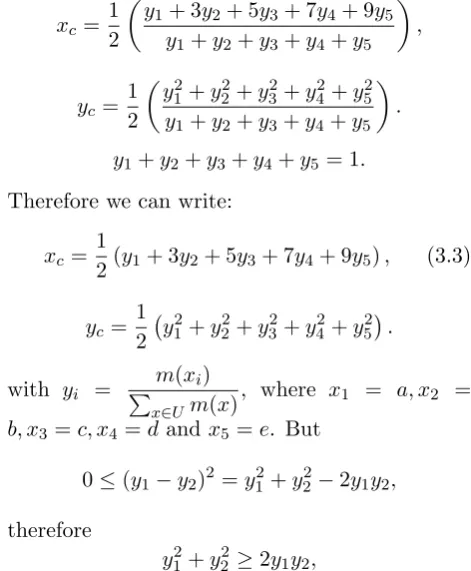
graph, it becomes evident that the transition from (3.1) to (3.2) is obtained under the assump-tion that all the intervals have length equal to 1 and that the first of them is the interval [0,1]. In our case (n= 5) formulas (3.2) are transformed into the following form:
xc= 1 2
(
y1+ 3y2+ 5y3+ 7y4+ 9y5
y1+y2+y3+y4+y5 )
,
yc= 1 2
(
y12+y22+y32+y24+y25 y1+y2+y3+y4+y5
) .
y1+y2+y3+y4+y5= 1.
Therefore we can write:
xc= 1
2(y1+ 3y2+ 5y3+ 7y4+ 9y5), (3.3)
yc= 1 2 (
y21+y22+y32+y24+y25).
with yi =
m(xi) ∑
x∈Um(x)
, where x1 = a, x2 =
b, x3=c, x4 =dand x5 =e. But
0≤(y1−y2)2 =y12+y22−2y1y2,
therefore
y12+y22≥2y1y2,
with the equality holding if, and only if,y1 =y2.
In the same way one finds that
y12+y32≥2y1y3,
and so on. Hence it is easy to check that
(y1+y2+y3+y4+y5)2 ≤5(y21+y22+y23+y42+y52),
with the equality holding if, and only ify1=y2=
y3 = y4 = y5. But y1 +y2 +y3 +y4 +y5 = 1,
therefore
1≤5(y12+y22+y23+y24+y52) (3.4)
with the equality holding if, and only ify1=y2=
y3 =y4 =y5 =
1 5.
Then the first of formulas (3.3) gives thatxc= 5 2. Further, combining the inequality (3.4) with the second of formulas (3.3) one finds that Therefore the unique minimum for yc corresponds to the
centre of mass Fm( 5 2,
1 10).
The ideal case is when y1 = y2 = y3 = y4 = 0
and y5 = 1. Then from formulas (3.3) we get
that xc= 9
2 and yc= 1
2. Therefore the centre of mass in this case is the pointFi(
9 2,
1 2).
On the other hand the worst case is when y1= 1
and y2 = y3 = y4 = y5 = 0. Then for formulas
(3.3) we find that the centre of mass is the point
Fw( 1 2,
1 2).
Therefore the ”area” where the centre of massFc lies is represented by the triangle Fw Fm Fi of Figure 3. Then from elementary geometric
con-Figure 3: Graphical representation of the ”area” of the centre of mass
siderations it follows that for two groups of a sys-tem’s objects with the same xc ≥ 2.5 the group having the centre of mass which is situated closer toFi is the group with the higher yc; and for two groups with the same xc <2.5 the group having the centre of mass which is situated farther toFw is the group with the loweryc.
formulate our criterion for comparing the groups performances in the following form:
• Among two or more groups the group with the biggestxcperforms better.
• If two or more groups have the samexc≥2.5, then the group with the higher yc performs better.
• If two or more groups have the samexc<2.5, then the group with the lower yc performs better.
From the above description it becomes clear that the application of the ’centroid’ method in prac-tice is simple and evident and needs no compli-cated calculations in its final step. However, we must emphasize that this method treats differ-ently the idea of a system’s performance, than the two measures of uncertainty presented above do. In fact, the weighted average plays the main role in this method, i.e. the result of the system’s performance close to its ideal performance has much more weight than the one close to the lower end. In other words, while the measures of uncer-tainty are dealing with the average systems per-formance, the ’centroid’ method is mostly looking at the quality of the performance. Consequently, some differences could appear in evaluating a sys-tems performance by these different approaches. Therefore, it is argued that a combined use of all these (3 in total) measures could help the user in finding the ideal profile of the system’s perfor-mance according to his/her personal criteria of goals.
4
Modelling
the
process
of
Problem Solving (PS)
In earlier papers we have developed models simi-lar to the general fuzzy model developed above for a more effective description of several situations involving fuzziness and uncertainty in the areas of Education (for the processes of Learning and of Mathematical modelling), of Artificial Intelli-gence (for Case-Based and Analogical Reasoning) and of Management (for the evaluation of the fuzzy data obtained by a markets research and for Decision Making); see for example [26] and its ref-erences. Notice also, that Subbotin et al., based on our fuzzy model for the process of learning
[21], have applied the ’centroid’ method on com-paring students’ mathematical learning abilities [16] and for measuring the scaffolding (assistance) effectiveness provided by the teacher to students [17]. Also Perdikaris has used the total possiblis-tic uncertainty [8] and the Shannon’s entropy [9] for assessing students geometrical reasoning skills in terms of the corresponding van Hieles’ levels. In this paper we shall apply our general fuzzy model developed above for representing the Prob-lem Solving (PS) process.
As the world economy moved from an industrial to a knowledge economy, it can be argued that the nature of many problems also changed and new problems have arisen which may require a differ-ent approach to overcome them. Educational in-stitutions and governments have recognized long ago the importance of PS and volumes of research have been written about PS (see [3], [7], etc). Universities and other higher learning institutions are entrusted with the task of producing gradu-ates that have such higher order thinking skills among other skills (e.g. see [1], etc).
Mathematics by its nature is a subject whereby PS forms its essence. According to Schoenfeld [14] a problem is only a problem (as mathemati-cians use the word) if you don’t know how to go about solving it. A problem that has no ’sur-prises’ in store, and can be solved comfortably by routine or familiar procedures (no matter how difficult!) it is an exercise. In an earlier paper [25][25] we have examined the role of problem in learning mathematics and we have attempted a review of the evolution of research on PS in math-ematics education from its emergency as a self sufficient science at the end of the 1960’s until to-day. Here is a rough chronology of that progress: 1950’s 1960’s: Polya’s theories on the use of heuristic strategies in PS ([10], etc)
1970’s: Emergency of mathematics education as a self sufficient science (research methods were almost exclusively statistical). Research on PS was mainly based on Polya’s ideas.
1980’s: A framework describing the PS process, and reasons for success or failure in PS (e.g. [6], [13], etc.)
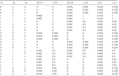
Table 1: Profiles with non zero membership degrees (The outcomes of the above Table were obtained with accuracy up to the third decimal point).
A1 A2 A3 Ms(1) rs(1) Ms(2) rs(2) f(s) r(s)
b b b 0 0 0.016 0.258 0.016 0.129
b b a 0 0 0.016 0.258 0.016 0.129
b a a 0 0 0.016 0.258 0.016 0.129
c c c 0.062 1 0.062 1 0.124 1
c c a 0.062 1 0.062 1 0.124 1
c c b 0 0 0.031 0.5 0.031 0.25
c a a 0 0 0.031 0.5 0.031 0.25
c b a 0 0 0.031 0.5 0.031 0.25
c b b 0 0 0.031 0.5 0.031 0.25
d d a 0.016 0.258 0 0 0.016 0.129
d d b 0.016 0.258 0 0 0.016 0.129
d d c 0.016 0.258 0 0 0.016 0.129
d a a 0 0 0.016 0.258 0.016 0.129
d b a 0 0 0.016 0.258 0.016 0.129
d b b 0 0 0.016 0.258 0.016 0.129
d c a 0.031 0.5 0.031 0.5 0.062 0.5
d c b 0.031 0.5 0.031 0.5 0.062 0.5
d c c 0.031 0.5 0.031 0.5 0.062 0.5
e c a 0.031 0.5 0 0 0.031 0.25
e c b 0.031 0.5 0 0 0.031 0.25
e c c 0.031 0.5 0 0 0.031 0.25
e d a 0.016 0.25 0 0 0.016 0.129
e d b 0.016 0.25 0 0 0.016 0.129
e d c 0.016 0.25 0 0 0.016 0.129
on analyzing the PS process and on describing the proper heuristic strategies to be used in each of its stages, more recent investigations have fo-cused mainly on solvers’ behavior and required attributes during the PS process; e. g. [2], [15], etc.
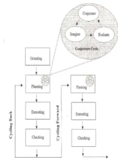
Carlson Bloom [2] drawing from the large amount of literature related to PS developed a broad taxonomy to characterize major PS at-tributes that have been identifying as relevant to PS success. This taxonomy gave genesis to their ’Multidimensional Problem-Solving Framework’ (MPSF), which includes the following 4 phases: Orientation, Planning, Executing and Checking. It has been observed that once the solvers ori-ented themselves to the problem space, the plan-execute-check cycle was usually repeated through out the remainder of the solution process; only in a few cases a solver obtained linearly the solution of a problem (i.e. he/she made this cycle only once). Thus embedded in the framework are two cycles (one cycling back and one cycling forward), each of which includes the three out of the four phases, that is planning, executing and checking.
It has been also observed that, when contemplat-ing various solution approaches durcontemplat-ing the plan-ning phase of the PS process, the solvers were at times engaged in a conjecture-imagine-evaluate (accept/reject) sub-cycle. Therefore, apart of the two main cycles, embedded in the framework is the above sub-cycle, which is connected to the phase of planning (see Figure 4, taken from [2]).
In order to illustrate the use of our results in practice, we performed the experiments presented in the next section.
5
Applications of the model for
PS
Figure 4: A graphical representation of Carlsons and Blooms MPSF
to students emphasizing among the others that we are interested for all their efforts (successful or not) during the PS process, and therefore they must keep records on their papers for all of them, at all stages of the PS process. This manipula-tion enabled as in obtaining realistic data from our experiment for each stage of the PS process and not only those based on students final results that could be obtained in the usual way of grad-uating their papers.
Our characterizations of students performance at each stage of the PS process involved:
• Negligible success, if they obtained (at the par-ticular stage) positive results for less than 2 problems.
• Low success, if they obtained positive results for 2, 3, or 4 problems.
• Intermediate success, if they obtained positive results for 5, 6, or 7 problems.
• High success, if they obtained positive results for 8, or 9 problems.
• Complete success, if they obtained positive re-sults for all problems.
A1 = {(a,0),(b,0),(c,0.5),(d,0.25),(e,0,0.25)},
In the same way we represented the stages of ex-ecuting and checking as fuzzy sets in U by A2 ={(a,0),(b,0),(c,0,5),(d,0,25),(e,0)}
and
A3 ={(a,0,25),(b,0,25),(c,0,25),(d,0),(e,0)}
respectively.
Next we calculated the membership degrees of the
53(ordered samples with replacement of 3 objects
taken from 5) in total possible students’ profiles as it is described in section2(column ofms(1) in Table1). For example, for the profiles= (c, c, a) one finds that ms = mA1(c).mA2(c).mA3(a) =
0,5.0,5.0,25) = 0,06225.
It is a straightforward process then to calculate in terms of the membership degrees the Shan-nons entropy for the student group, which is H ≈0,289.
Further, from the values of the column of ms(1) it turns out that the maximal membership de-gree of students’ profiles is 0,06225. Therefore the possibility of each sinU3 is given by
rs= ms 0.06225.
Calculating the possibilities of all profiles (column of rs(1) in Table 1) one finds that the ordered possibility distribution for the student group is:
r :r1 =r2 = 1, r3 =r4 =r5=r6 =r7 =r8= 0.5,
r9 =r10=r11=r12=r13=r14= 0.258,
r15=r16=· · ·=r125 = 0.
Thus with the help of a calculator one finds that
ST(r) = 1 log2
[14 ∑
i=1
(ri−ri+1)log
i ∑i
j=1rj ]
≈ 1 0.301
[
0.5log2
2 + 0.242log 8
5+ 0.258log 14 6.548
]
≈3,32.0,242.0,204 + 0,258.0,33≈0.445 and
N(r) = 1 log2
[14 ∑
i=1
(ri−ri+1)logi ]
= 1
log2(0.5log2 + 0.242log8 + 0.258log14)
Therefore we finally have thatT(r)≈2,653. A few days later we performed the same experi-ment with a group of 30 students of the School of Management and Economics. Working as above we found that
A1 ={(a,0),(b,0,25),(c,0,5),(d,0,25),(e,0)},
A2 ={(a,0,25),(b,0,25),(c,0,5),(d,0),(e,0)}
A3 ={(a,0,25),(b,0,25),(c,0,25),(d,0),(e,0)}
which isH ≈0,312.
Since the maximal membership degree is again 0,06225, the possibility of each s is given by the same formula as for the first group. Calculating the possibilities of all profiles (column of rs(2) in Table1) one finds that the ordered possibility distribution of the second group is:
r:r1 =r2 = 1, r3 =r4 =r5=r6=r7 =r8 = 0.5,
r9 =r10=r11=r12=r13=r14= 0.258,
r15=r16=· · ·=r125= 0.
Finally, working in the same way as above one finds thatT(r) = 0,432 + 2,179 = 2,611. There-fore, since 2,611 < 2,653, it turns out that the second group had in general a slightly better per-formance than the first one. Notice that the val-ues of the Shannon’s entropy lead to the oppo-site conclusion (since 0,312¿0,289), but this, as we have already explained in section2, is not sur-prising in cases, where the difference between the performances of the two groups is very small. Further, using formulas (3.3) of section3, one can compare the performances of the two groups by the ’centroid’ method in each of the listed above phases of the PS process as follows:
Denote byAij the fuzzy subset of U attached to the phase Sj, j = 1,2,3 , of theP S process with respect to the student groupi, i= 1,2.
In the first phase of orientation/planning we have A11={(a,0),(b,0),(c,0,5),(d,0,25),(e,0,25)},
A21={(a,0),(b,0,25),(c,0,5),(d,0,25),(e,0)}
and respectively
xc11=
1
2(5.0,5 + 7.0,25 + 9.0,25) = 3,25
xc21=
1
2(3.0,25 + 5.0,5 + 7.0,25) = 2,25 . By our criterion the first group demonstrates better performance. At the second stage of solu-tion we have:
A11={(a,0),(b,0),(c,0,5),(d,0,25),(e,0)},
A21={(a,0,25),(b,0,25),(c,0,5),(d,0),(e,0)}.
A11={(a,0),(b,0),(c,0,67),(d,0,33),(e,0)},
A21={(a,0,25),(b,0,25),(c,0,5),(d,0),(e,0)}.
and respectively
xc12=
1
2(5.0,67 + 7.0,33) = 5,66
xc22=
1
2(0,25 + 3.0,25 + 5.0,25) = 3,25
. By our criterion the first group demonstrates again a significantly better performance. Finally, at the third phase of checking we have
A13=A23=
(a,0,25),(b,0,25),(c,0,25),(d,0),(e,0),
which obviously means that in this phase the per-formances of both groups are identical. Based on our calculations we can conclude that the first group demonstrated a significantly better perfor-mance at the phases of orientation/planning and of executing, but performed identically with the second one at the phase of checking.
Remark 5.1 In earlier papers we have also de-veloped a stochastic model for the representation of the PS process by applying a Markov chain on the stages of Schoenfeld’s ’Expert Performance Model for PS’ ([19], [20]). There are many sim-ilarities between Carlson’s and Blum’s MPSF [2] and Schoenfeld’s model [13]. However, their main qualitative difference is that, while in the former case emphasis is given to the solver’s behaviour and required attributes rather, the latter is ori-ented towards the PS process itself (use of the proper heuristic strategies at each stage of the pro-cess).
Our stochastic model for the PS process is self restricted to give quantitative information only through the description of the ideal behavior of a group of solvers (i.e. how they must act for the solution of a problem and not how they really act in practice).
6
Conclusion
The following conclusions can be drawn from the discussion performed in this paper:
• In this paper we developed a general fuzzy model for representing processes in a sys-tems operation involving vagueness and/or uncertainty. We also presented 3 methods of measuring a systems effectiveness connected to the above model. The first of them con-cerns the measurement of the total possibilis-tic uncertainty defined on the systems pro-files ordered possibility distribution and be-ing equal to the sum of strife and non speci-ficity. The second concerns the measurement of the systems probabilistic uncertainty ex-pressed by a modified version of the Shan-nons entropy for use in a fuzzy environment. Finally, the third one is the, so called, cen-troid method, in which the coordinates of the center of mass of the graph of the member-ship function involved provide an alternative measure of the system’s performance. Each one of the above methods adheres its own ad-vantages and disadad-vantages and a combined use of them could help the user in finding the ideal profile of the systems performance ac-cording to his/her personal criteria of goals.
• In earlier papers we have applied similar fuzzy models for a more effective description of several processes in the areas of Education, of Artificial Intelligence and of Management. In the present paper we applied our general fuzzy model for the description of the PS process The construction of the fuzzy model for the PS process was based on Carlsons and Blums Multidimensional PS Framework (MPSF). Two classroom experiments were also presented illustrating the use of our re-sults in practice.
• In contrast to our stochastic (Markov chain) model for the PS process developed in ear-lier papers, which is restricted to give quan-titative information only, our fuzzy model has the advantage of giving also a qualita-tive/realistic view of the PS process through the calculation of the probabilities and/or possibilities of all possible solvers profiles. Nevertheless, the characterization of the problem solvers performance in terms of a set of linguistic labels, which are fuzzy them-selves, is a disadvantage of the fuzzy model, because this characterization depends on the users personal criteria. A live example about
this is the different evaluations for the two groups of solvers obtained by using our fuzzy measures for the PS skills in our classroom experiments presented in section 5. There-fore the stochastic could be used as a tool for the validation of the fuzzy model in the effort of achieving a worthy of credit mathe-matical analysis of the PS process.
Appendix
List of the problems given for solution to students in our classroom experiment
Problem 1: We want to construct a channel to run water by folding across its longer side the two edges of an orthogonal metallic leaf having sides of length 20cm and 32 cm, in such a way that they will be perpendicular to the other parts of the leaf. Assuming that the flow of the water is constant, how we can run the maximum possible quantity of the water?
Problem 2: Given the matrixA=
10 21 22 0 0 1
and a positive integern, find the matrixAn.
Problem 4: Let us correspond to each let-ter the number showing its order into the alphabet (A = 1, B = 2, C = 3etc). Let us cor-respond also to each word consisting of 4 letters
a 2X2 matrix (
19 15 13 5
)
corresponds to the
word SOME. Using the matrix E = (
8 5 11 7
)
as an encoding matrix how you could send the message LATE in the form of a camouflaged matrix to a receiver knowing the above process and how the receiver could decode your message?
Problem 5: The demand function P(Qd) = 25 − Q2d represents the different prices that consumers willing to pay for different quantities Qd of a good. On the other hand the supply function P(Qs) = 2Qs+ 1 represents the prices at which different quantities Qs of the same good will be supplied. If the markets equilibrium occurs at (Q0, P0), the producers who would
supply at lower price than P0 benefit. Find the total gain to producers.
corre-sponding ball to the box before the next lottery. Find the probability of getting all the balls that he draws out of the box different.
Problem 7: A box contains 3 white, 4 blue and 6 black balls. If we put out 2 balls, what is the probability of choosing 2 balls of the same colour?
Problem 9: A company circulates for first time in the market a new product, say K. Markets research has shown that the consumers buy on average one such product per week, either K, or a competitive one. It is also expected that 70i) Find the markets share for K two weeks after its first circulation, provided that the markets conditions remain unchanged.
ii) Find the markets share for K in the long run, i.e. when the consumers preferences will be stabilized.
Problem 10: Among all cylinders having a total surface of 180 m2, which one has the maximal volume?
Problem 10: Among all cylinders having a total surface of 180 m2, which one has the maximal volume?
References
[1] A. W. Astin, What matters in college? For critical years revisited, Jossey-Bass Inc., San Francisco, 1993.
[2] M. P. Carlson, I. Bloom, The cyclic na-ture of problem solving: An emergent multi-dimensional problem solving framework, Ed-ucational Studies in Mathematics 58 (2005) 45-75.
[3] D. F. Halpern, Critical thinking across the curriculum: A brief edition of thought and knowledge, Lawrence Erlbaum associates, London, 1997.
[4] G. J. Klir, T. A. Folger, Fuzzy Sets, Uncer-tainty and Information, Prentice-Hall, Lon-don, 1988.
[5] J. G. Klir, Principles of Uncertainty: What are they? Why do we mean them?, Fuzzy Sets and Systems 74 (1995) 15-31.
[6] F. K. Lester, J. Garofalo, D. L. Krol, Self-confidence, interest, beliefs and metacogni-tion: Key influences on problem-solving be-havior, in: D. B. Mcleod V. M. Adams (Eds),
Affect and Mathematical Problem Solving: A New Perspective, 75-88, Springer-Verlag, New York, 1989.
[7] National Council of Teachers of Math-ematics (NCTM), Principles and stan-dards of school mathematics, available at http://standards.nctm.org , 2010.
[8] S. Perdikaris,Measuring the student group ca-pacity for obtaining geometric information in the van Hiele development though process: A fuzzy approach, Fuzzy Sets and Mathematics 16 (2002) 81-86.
[9] S. Perdikaris, Using Fuzzy Sets to Determine the Continuity of the van Hiele Levels, Jour-nal of Mathematical Sciences and Mathemat-ics Education 6(2011) 39-46.
[10] G. Polya, How to solve it, Princeton Univ. Press, Princeton, 1945.
[11] G. L. S. Shackle, Decision, Order and Time in Human Affairs, Cambridge Univer-sity Press, Cambridge, 1961.
[12] C. E. Shannon, A mathematical theory of communications, Bell Systems Technical Journal 27 (1948) 379-423.
[13] A. Schoenfeld, Teaching problem solving skills, American Mathematical Monthly 87 (1980) 794-805.
[14] A. Schoenfeld, The wild, wild, wild world of problem solving: A review of sorts, For the Learning of Mathematics 3 (1983) 40-47.
[15] A. Schoenfeld, How we think: A theory of goal-oriented decision making and its educa-tional applications, N. Y. , Routledge, 2012.
[16] I. Subbotin, H. Badkoobehi, N. Bilotskii,
Application of Fuzzy Logic to Learning As-sessment, Didactics of Mathematics: Prob-lems and Investigations 22 (2004) 38-41.
[17] I. Subbotin, F. Mossovar-Rahmani, N. Bilot-skii,Fuzzy logic and the concept of the Zone of Proximate Development, Didactics of Math-ematics: Problems and Investigations 36 (2011) 101-108.
fuzzy system outputs defined on trapezoidal fuzzy partitions, Fuzzy Sets and Systems 157 (2006) 904-918.
[19] M. GR. Voskoglou, S. Perdikaris, A Markov Chain Model in Problem Solving, Interna-tional Journal of Mathematics Education in science and Technology 6 (1991) 909-914.
[20] M. Gr. Voskoglou, S. Perdikaris, Measuring Problem Solving Skills, International Jour-nal of Mathematics Education in Science and Technology 3 (1993) 443-447.
[21] M. Gr. Voskoglou, The process of learning mathematics: A fuzzy set approach, Heuristic and Didactics of Exact Sciences (Ukraine) 10 (1999) 9-13.
[22] M. Gr. Voskoglou, The use of mathematical modelling as a learning device of mathemat-ics, Quaderni di Ricerca in Didattica (Scienze Mathematiche), University of Palermo 16 (2006) 53-60.
[23] M. Gr. Voskoglou,The mathematics teacher in the modern society, Quaderni di Ricerca in Didattica (Scienze Mathematiche), University of Palermo 19 (2009) 24-30.
[24] M. Gr. Voskoglou,Fuzzy Sets in Case-Based Reasoning, Fuzzy Systems and Knowledge Discovery 6 (2009) 252-256, IEEE Computer Society.
[25] M. Gr. Voskoglou, Problem Solving from Polya to Nowadays: A Review and Future Perspectives. In R. V. Nata (Ed.), Progress in Education, Vol. 22, Chapter 4, 65-82, Nova Publishers, N. Y., 2011.
[26] M. Gr. Voskoglou,Stochastic and fuzzy mod-els in Mathematics Education, Artificial In-telligence and Management, Lambert Aca-demic Publishing, Saarbrucken, Germany, 2011 (for more details look at http://amzn. com./3846528218.)
[27] M. Gr. Voskoglou, I. Ya. Subbotin, Fuzzy Models for Analogical Reasoning, Interna-tional Journal of Applications of Fuzzy Sets 2 (2012) 19-38.
[28] L. A. Zadeh, Fuzzy Sets, Information and Control 8 (1965) 338-353.