Simple Speech Transform Coding Scheme using Forward Adaptive Quantization for Discrete Input Signal

(1)

Information Technology and Control 2019/3/48 454

Simple Speech Transform Coding

Scheme Using Forward Adaptive

Quantization for Discrete Input Signal

ITC 3/48

Journal of Information Technology and Control

Vol. 48 / No. 3 / 2019 pp. 454-463

DOI 10.5755/j01.itc.48.3.21685

Simple Speech Transform Coding Scheme Using Forward

Adaptive Quantization for Discrete Input Signal

Received 2018/09/19 Accepted after revision 2019/08/02

http://dx.doi.org/10.5755/j01.itc.48.3.21685

Corresponding author: [email protected]

Zoran Perić, Milan Tančić, Nikola Simić

Faculty of Electronic Engineering, University of Niš, Department of Telecommunications, Serbia, Aleksandra Medvedeva 14, 18000, Niš, Serbia; e-mails: [email protected], [email protected], [email protected]

Vladimir Despotović

University of Belgrade, Technical Faculty in Bor, Vojske Jugoslavije 12, 19210 Bor, Serbia; e-mail: [email protected]

The speech coding scheme based on the simple transform coding and forward adaptive quantization for dis-crete input signal processing is proposed in this paper. The quasi-logarithmic quantizer is applied for discreti-zation of continuous input signal, i.e. for preparing discrete input. The application of forward adaptation based on the input signal variance provides more efficient bandwidth usage, whereas utilization of transform coding provides sub-sequences with more predictable signal characteristics that ensure higher quality of signal re-construction at the receiving end. In order to provide additional compression, transform coding precedes adap-tive quantization. As an objecadap-tive measure of system performance, signal-to-quantization-noise ratio is used. System performance is discussed for two typical cases. In the first case, it was considered that the information about continuous signal variance is available, whereas the second case considers system performance estima-tion when only the informaestima-tion about discretized signal variance is present, which means that there is a loss of input signal information. The main goal of such performance estimation comparison of the proposed speech signal coding model is to explore what is the objectivity of performance if the information about a continuous source is absent, which is a common phenomenon in digital systems. The advantages of the proposed coding scheme are demonstrated by comparing the performance of the reconstructed signal with other similar exiting speech signal coding systems.

(2)

1. Introduction

Quantization represents the process of mapping the range of signal amplitude values, which can be contin-uous and infinite in general, into a set of discrete val-ues and it represents a core method exploited in sig-nal processing algorithms. It is an indispensable part of “lossy” signal compression algorithms, which may incorporate additional coding techniques to manipu-late the presentation of a signal in digital domain. A constant need for solutions of less complexity, which would require the usage of lower bit-rates but keeping the high quality of reconstructed signal, is a demand-ing challenge with the rapid growth of information systems [10], [4], [11], [31], [28]. Quantization is the process of preparing a signal in digital domain and making it suitable for processing by a computer or any digital circuit [9]. Considering the growing interest in man-machine communication, speech and voice recognition is considered as important [37], [23-24], [36], [7], [16], [25]. Recent research and applications, which exploit neural networks, commonly incorpo-rate quantization of weight coefficients and activa-tion funcactiva-tions. It is shown that scalar quantizaactiva-tion is suitable for such task as well as for speech recognition algorithms using deep convolutional neural networks [35], [13]. This paper proposes a speech signal coding scheme with scalar quantization implemented, where every sample of input signal is processed separately using scalar quantizers [6]. Such an approach is less complex than a vector quantization based approach, which processes input signal samples grouped into the vectors (arrays) and where vectors are quantized at once [35], [20].

For non-stationary signals coding, such as speech sig-nal, the usage of adaptive schemes increases quality of reconstructed signal in the manner of adapting quan-tizer design to the varying statistics of an input signal frame (mean value or variance typically) to achieve better performances. More efficient bandwidth usage of the original samples can be provided by including transform coding algorithms into the coding scheme [14-15], which is a part of several standards in the field of high quality wideband speech/audio coding [19]. Some of the most well-known transforms are discrete wavelet transform (DWT) [17], [34], [12], discrete cosine transform (DCT) [8], [26], Karhunen-Loeve transform (KLT) [2-3] and Hadamard transform [33].

In this paper, we analyze and propose a trans-form-based adaptive coding scheme based on for-ward adaptive quantization in the case of discrete input signal. The coding process presented in the pro-posed scheme can be observed as a two stage coding. Firstly, the continuous signal is discretized using a quasi-logarithmic quantizer Q0, which forms

ampli-tude limited discrete signal that is further coded in the stage two. The amplitude limitation of discret-ized signal causes the absence of overload distortion, which is disregarded in the processing of further step. In the second stage, discretized signal is encod-ed using a simple transform coding that decompos-es wideband speech signal into sub-sequencdecompos-es with narrower bandwidth range and it is adapted using a forward adaptation technique. The aim of such transform-based coding step is to provide additional compression before adaptive quantization [32], [30]. After that, speech signal is divided into frames whose size is 240 samples, which are further adapted to the variance framewise [5], [27], [21]. Since the forward adaptation is used, the variance is quantized using the log-uniform quantizer and this information is trans-ferred to the receiver [18].

The proposed coding scheme shows suitability for speech signal coding as it provides 4.9 – 7.8 [dB] of gain comparing to the results which provide the usage of quasi-logarithmic quantizer in the second stage [29], and up to 10 [dB] of gain comparing to the results which provide the usage of uniform quantizer in the first and optimal comandor in the second stage [22]. The remaining of the paper is organized as follows: in Section 2, a detailed description of the proposed quantizer model is provided. Next, numerical results and discussion are presented in Section 3. In the end, concluding remarks are summed up in Section 4.

2. Quantizer Design for Discrete

Input Signal

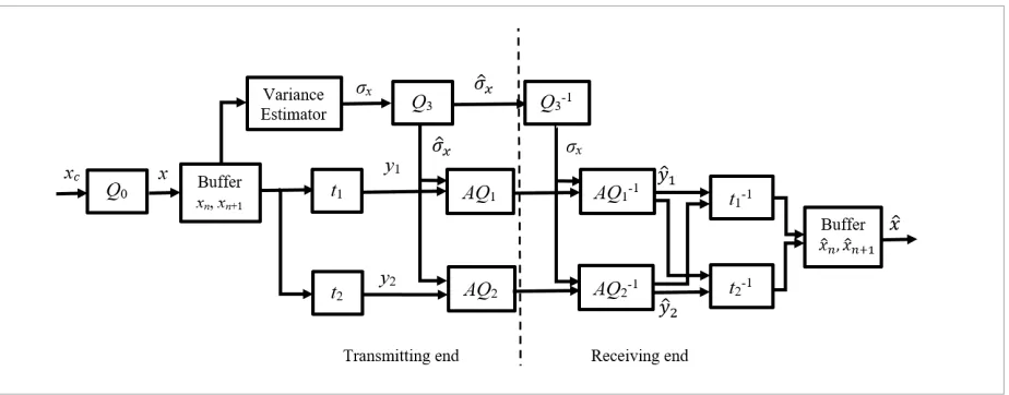
The proposed coding scheme is shown in Fig. 1. It can be seen that the encoder is composed of a qua-si-logarithmic quantizer Q0, which is exploited for

(3)

Information Technology and Control 2019/3/48 456

buffer, variance estimator, transform encoder and for-ward-adaptive quasi-logarithmic quantizers AQ1 and AQ2. The purpose of quasi-logarithmic quantizer Q0

(R0=8 [bits/sample], µ=255) is to obtain discrete

sam-ples of continuous input speech signal that is further fed into the buffer. Although a robust quasi-logarith-mic quantizer is used, significant errors may occur for higher values of variance due to range mismatch, resulting a huge difference of estimated performance between the cases where the information about con-tinuous signal is available and when the information about discrete signal only is achievable. If the wide range of variances is observed, it is not enough to ex-ploit only one robust quantizer Q0, but it is necessary

to use two quantizers in pre-processing, where one will cover processing of lower bands range while an-other will be used for processing signals of upper band range variances. On the other hand, if uniform quan-tizers are exploited, which are known as not robust, system performance would be much worse. Such an analysis has not been done before, and it is therefore considered as a significant step forward in the field. After discretizing continuous signal, discretized signal is fed to the buffer which is used to divide signal into frames. Consequently, further signal processing is not anymore sample-based but frame-based. Next, simple transforms t1 and t2 are applied to form two

sub-se-quences y1 and y2, creating two independent signals

with more predictable characteristics. These

trans-forms are defined similarly as Hadamard transform for a group of two samples and their form is [32], [30]: (DCT) [8], [26], Karhunen-Loeve transform (KLT)

[2-3] and Hadamard transform [3[2-3].

In this paper, we analyze and propose a transform-based adaptive coding scheme transform-based on forward adaptive quantization in the case of discrete input signal. The coding process presented in the proposed scheme can be observed as a two stage coding. Firstly, the continuous signal is discretized using a quasi-logarithmic quantizer Q0, which forms amplitude

limited discrete signal that is further coded in the stage two. The amplitude limitation of discretized signal causes the absence of overload distortion, which is disregarded in the processing of further step. In the second stage, discretized signal is encoded using a simple transform coding that decomposes wideband speech signal into sub-sequences with narrower bandwidth range and it is adapted using a forward adaptation technique. The aim of such transform-based coding step is to provide additional compression before adaptive quantization [32], [30]. After that, speech signal is divided into frames whose size is 240 samples, which are further adapted to the variance framewise [5], [27], [21]. Since the forward adaptation is used, the variance is quantized using the log-uniform quantizer and this information is transferred to the receiver [18].

The proposed coding scheme shows suitability for speech signal coding as it provides 4.9 – 7.8 [dB] of gain comparing to the results which provide the usage of quasi-logarithmic quantizer in the second stage [29], and up to 10 [dB] of gain comparing to the results which provide the usage of uniform quantizer in the first and optimal comandor in the second stage [22].

The remaining of the paper is organized as follows: in Section 2, a detailed description of the proposed quantizer model is provided. Next, numerical results and discussion are presented in Section 3. In the end, concluding remarks are summed up in Section 4.

2. Quantizer Design for Discrete Input Signal

The proposed coding scheme is shown in Fig. 1. It can be seen that the encoder is composed of a quasi-logarithmic quantizer Q0, which is exploited for

discretization of continuous input speech signal, then buffer, variance estimator, transform encoder and forward-adaptive quasi-logarithmic quantizers AQ1

and AQ2. The purpose of quasi-logarithmic quantizer

Q0 (R0=8 [bits/sample], µ=255) is to obtain discrete

samples of continuous input speech signal that is further fed into the buffer. Although a robust quasi-logarithmic quantizer is used, significant errors may occur for higher values of variance due to range mismatch, resulting a huge difference of estimated performance between the cases where the information about continuous signal is available and when the information about discrete signal only is achievable. If the wide range of variances is observed, it is not enough to exploit only one robust quantizer Q0, but it

is necessary to use two quantizers in pre-processing, where one will cover processing of lower bands range while another will be used for processing signals of upper band range variances. On the other hand, if uniform quantizers are exploited, which are known as not robust, system performance would be much worse. Such an analysis has not been done before, and it is therefore considered as a significant step forward in the field.

After discretizing continuous signal, discretized signal is fed to the buffer which is used to divide signal into frames. Consequently, further signal processing is not anymore sample-based but frame-based. Next, simple transforms t1 and t2 are applied to form two

sub-sequences y1 and y2, creating two independent signals

with more predictable characteristics. These transforms are defined similarly as Hadamard transform for a group of two samples and their form is [32], [30]:

( )

2

: 1 1

1 y = xn+xn+

t , (1)

( )

,

2

: 1

2

2 y = xn−xn+

t (2)

where xn and xn+1 are neighboring samples of the input

signal, while y1 and y2 represent samples of

transformed signal. These transformed signals have variances σ₁₂ andσ₂₂ , respectively, whose values depend on the discrete input signal variance σx2 and

correlation coefficient ρ [30]:

(

1

)

, 2

2 2

1 =σ +ρ

σ x (3)

(

1

)

. 2

2 2

2 =σ −ρ

σ x ₍₄₎

Such transformed sequences are independent and are further encoded separately using quantizers with forward adaptation applied (AQ1 and AQ2).

(1) (DCT) [8], [26], Karhunen-Loeve transform (KLT)

2. Quantizer Design for Discrete Input Signal

( )

2

: 1 1

1 y = xn+xn+

t , (1)

( )

,

2

: 2 1

2 y = xn−xn+

t (2)

(

1

)

, 2

2 2

1 = σ +ρ

σ x (3)

(

1

)

. 2

2 2

2=σ −ρ

σ x (4)

(2)

where xn and xn+1 are neighboring samples of the

in-put signal, while y1 and y2 represent samples of

trans-formed signal. These transtrans-formed signals have vari-ances σ12 and σ22, respectively, whose values depend

on the discrete input signal variance σx2 and

correla-tion coefficient ρ [30]: (DCT) [8], [26], Karhunen-Loeve transform (KLT)

2. Quantizer Design for Discrete Input Signal

( )

2

: 1 1

1 y = xn+xn+

t , (1)

( )

,

2

: 2 1

2 y = xn−xn+

t (2)

(

1

)

, 2

2 2

1 = σ +ρ

σ x ₍₃₎

(

1

)

. 2

2 2

2 =σ −ρ

σ x (4)

(3) (DCT) [8], [26], Karhunen-Loeve transform (KLT)

2. Quantizer Design for Discrete Input Signal

( )

2

: 1

1

1 y = xn+xn+

t , (1)

( )

,

2

: 1

2

2 y = xn−xn+

t (2)

(

1

)

, 2

2 2

1 = σ +ρ

σ x (3)

(

1

)

. 2

2 2

2=σ −ρ

σ x (4)

(4)

Such transformed sequences are independent and are further encoded separately using quantizers with for-ward adaptation applied (AQ1 and AQ2).

In order to achieve higher quality of reconstructed signal, adaptive quantization based on the variance of the signal has been performed in the next step [15], [27]. Firstly, frames that consist of M samples of input signal are being loaded into the buffer. The variance of

Figure 1

The proposed speech coding scheme for discrete input signal

Figure 1. The proposed speech coding scheme for discrete input signal

In order to achieve higher quality of reconstructed signal, adaptive quantization based on the variance of the signal has been performed in the next step [15], [27]. Firstly, frames that consist of M samples of input signal are being loaded into the buffer. The variance of M samples in a frame is calculated by using variance estimator, then quantized by using log-uniform quantizer Q3 and after that it is transmitted to the

receiving end. It should be noted that log-uniform quantizer is actually uniform quantizer designed in logarithmic domain which is described in details in [15], [27]. Next, variance quantized this way is sent to adaptive quantizers AQ1 and AQ2 for support range

determination for each frame using the following expressions: ( ) ( ) , 2 1 ˆ mL 1 max       +ρ ⋅ σ ⋅ =x

x AQ i (5)

( )

( 2 ) mL ˆ 1₂ , max =x ⋅σ⋅ _ −ρ_

x AQ i (6)

where σˆ represents quantized standard deviation, ρ is correlation coefficient of the input signal whereas xmL

is initial support range value of quantizer designed for Laplacian source with the unit variance, compression factor µ and N quantization levels [30], [1].

Quasi-logarithmic quantizers used in the proposed model (AQ1, AQ2, and Q0) are designed using the µ

-logarithmic compression law, whose compression function is defined as [10], [27]:

( ) ₍ ₎ln1 sgn( ), ,

1

ln max max

max _x _x _x

x x x

x

c _ ≤

      µ + µ + = (7)

where xmax is the support range of the quantizer,

whereas μ is the compression factor. According to the

μ-logarithmic compression function, decision

thresholds xi′ and representation levels yi′ are obtained

[10], [27].

Commonly, a logarithmic quantizer is suitable to use for middle and high bit-rates (N ≥ 8) [10], [27]. As the quasi-logarithmic quantizers are exploited for both

signals, y1 and y2, the quantizers AQ1 and AQ2 are

designed for bit-rates defined as [27]:

( )

. log 2 1 1 1 2 2 2

∏

= σ σ + = M k M k t t R R (8)

Equation (8) represents general expression for obtaining optimal bit-rate where M is the total number of branches (independent sub-sequences), whereas t can take values 1 or 2 for the proposed model (branches 1 and 2), while k presents counter through the branches. Consequently, the optimal values of R1

and R2 (AQ1 and AQ2, respectively) for the proposed

coding scheme could be defined as:

, 1 1 log 4 1 2 1=R+ +₋_ρρ

R (9) . 1 1 log 4 1 2 2=R+ ₊−_ρρ

R (10)

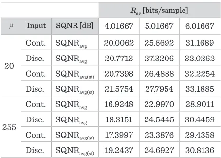
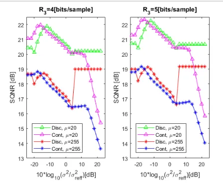
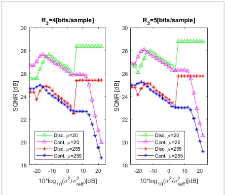
Among other common objective performance measures, in this paper we observe the signal-to-quantization-noise ratio (SQNR) which is calculated for the proposed coding scheme by using a modified model that have been proposed in [29]. Estimation is performed such that the input signal is divided firstly into frames of M samples in order to calculate signal dynamics, by determining the highest and lowest variance of a frame as:

( ) ( ) , log 10 ] dB [ ₂ min 2 max         σ σ ⋅ = M M B (11)

where 2

max

σ and 2

min

σ represent highest and lowest signal variances, respectively, whereas B denotes signal dynamics. In order to provide an adequate comparison, referent variance is equal to 0 [dB], as it is a common case, and it is chosen at the half of the dynamic range, limited by σ2_max_and_σ2_min_{. The whole}

(4)

457

Information Technology and Control 2019/3/48

M samples in a frame is calculated by using variance estimator, then quantized by using log-uniform quan-tizer Q3 and after that it is transmitted to the receiving

end. It should be noted that log-uniform quantizer is actually uniform quantizer designed in logarithmic domain which is described in details in [15], [27]. Next, variance quantized this way is sent to adaptive quantizers AQ1 and AQ2 for support range

determina-tion for each frame using the following expressions:

M samples in a frame is calculated by using variance estimator, then quantized by using log-uniform quantizer Q3 and after that it is transmitted to the

x AQ i (5)

( )

( ₂ ) mL ˆ 1₂ ,

max =x ⋅σ⋅ _ −ρ_

x AQ i (6)

where

σ

ˆ

represents quantized standard deviation, ρ is correlation coefficient of the input signal whereas xmL

( )

₍

₎

ln1 sgn

( )

, ,

1

lnmax x_max x x xmax

x x

x

c _ ≤

      µ + µ + = (7)

μ-logarithmic compression function, decision thresholds xi′ and representation levels yi′ are obtained [10], [27].

( )

. log 2 1 1 1 2 2 2

∏

= σ σ + = M k M k t t R R (8)

Equation (8) represents general expression for obtaining optimal bit-rate where M is the total number of branches (independent sub-sequences), whereas t

can take values 1 or 2 for the proposed model (branches 1 and 2), while k presents counter through the branches. Consequently, the optimal values of R1

, 1 1 log 4 1 2 1=R+ ₋+_ρρ

R (9) . 1 1 log 4 1 2 2=R+ ₊−ρ_ρ

R (10)

( )

, log 10 ] dB [ ₂ min 2 max         σ σ ⋅ = M M B (11)

where

σ

max2 and

σ

min2 represent highest and lowest signal variances, respectively, whereas B denotes signal dynamics. In order to provide an adequate comparison, referent variance is equal to 0 [dB], as it is a common case, and it is chosen at the half of the dynamic range, limited by σ2_max_and_σ2_min_{. The whole}

range B=60 [dB] (-30 to 30 [dB]) is divided into the segments with 2 [dB] step size, whereas input signal is (5)

x AQ i (5)

( )

( ₂ ) mL ˆ 1₂ ,

max =x ⋅σ⋅ _ −ρ_

x AQ i (6)

where

σ

ˆ

( )

₍

₎

ln 1 sgn

( )

, , 1

x x

x

c _ ≤

      µ + µ + = (7)

μ-logarithmic compression function, decision thresholds xi′ and representation levels yi′ are obtained

[10], [27].

( )

. log 2 1 1 1 2 2 2

∏

= σ σ + = _M k M k t t R R (8)

, 1 1 log 4 1 2 1=R+ ₋+_ρρ

R (9) . 11 log 4 1 2 2=R+ ₊−_ρρ

R (10)

( )

where

σ

max2 and

σ

where

σ

ˆ

Quasi-logarithmic quantizers used in the proposed model (AQ1, AQ2, and Q0) are designed using the

µ-logarithmic compression law, whose compression function is defined as [10], [27]:

determination for each frame using the following expressions:

( )

( ₁ ) mL ˆ 1₂ ,

max       +ρ ⋅ σ ⋅ =x

x _AQ _i (5)

( )

( ₂ ) mL ˆ 1₂ ,

max =x ⋅σ⋅ _ −ρ_

x AQ i (6)

where

σ

ˆ

( )

₍

₎

ln1 sgn

( )

, ,

1

ln max max

max _x _x _x

x x x

x

c _ ≤

      µ + µ + = (7)

whereas μ is the compression factor. According to the μ-logarithmic compression function, decision thresholds xi′ and representation levels yi′ are obtained

[10], [27].

( )

. log 2 1 1 1 2 2 2

∏

= σ σ + = M k M k t t R R (8)

, 1 1 log 4 1 2 1=R+ ₋+_ρρ

R (9) . 1 1 log 4 1 2 2=R+ ₊−_ρρ

R (10)

( )

where 2 max

σ

and 2 min

σ

represent highest and lowest signal variances, respectively, whereas B denotes signal dynamics. In order to provide an adequate comparison, referent variance is equal to 0 [dB], as it is a common case, and it is chosen at the half of the dynamic range, limited by σ2_max_and_σ2_min_{. The whole}

whereas μ is the compression factor. According to the μ-logarithmic compression function, decision thresholds xi′ and representation levels yi′ are

ob-tained [10], [27].

Commonly, a logarithmic quantizer is suitable to use for middle and high bit-rates (N ≥ 8) [10], [27]. As the quasi-logarithmic quantizers are exploited for both signals, y1 and y2, the quantizers AQ1 and AQ2 are

de-signed for bit-rates defined as [27]: Figure 1. The proposed speech coding scheme for discrete input signal

( )

( ₁ ) mL ˆ 1₂ ,

max       +ρ ⋅ σ ⋅ =x

x _AQ _i (5)

( )

( ₂ ) mL ˆ 1₂ , max =x ⋅σ⋅ _ −ρ_

x AQ i (6)

where

σ

ˆ

( )

₍

₎

ln1 sgn

( )

, ,

1

ln max max

max _x _x _x

x x x

x

c _ ≤

      µ + µ + = (7)

whereas μ is the compression factor. According to the μ-logarithmic compression function, decision thresholds xi′ and representation levels yi′ are obtained

[10], [27].

( )

. log 2 1 1 1 2 2 2

∏

= σ σ + = M k M k t t R R (8)

, 1 1 log 4 1 2 1=R+ ₋+_ρρ

R (9) . 1 1 log 4 1 2 2=R+ ₊−_ρρ

R (10)

( )

where 2 max

σ

and 2 min

σ

range B=60 [dB] (-30 to 30 [dB]) is divided into the segments with 2 [dB] step size, whereas input signal is

(8)

Equation (8) represents general expression for ob-taining optimal bit-rate where M is the total number

of branches (independent sub-sequences), whereas t

can take values1 or 2 for the proposed model (branch-es 1 and 2), while k presents counter through the branches. Consequently, the optimal values of R₁ and

R2 (AQ1 and AQ2, respectively) for the proposed

cod-ing scheme could be defined as: Figure 1. The proposed speech coding scheme for discrete input signal

determination for each frame using the following expressions: ( ) ( ) , 2 1 ˆ mL 1

max =x ⋅σ⋅ _ +ρ_

x AQ i (5)

( ) ( ) , 2 1 ˆ mL 2

max =x ⋅σ⋅ _ −ρ_

x AQ i (6)

where

σ

ˆ

( )

₍

₎

ln1 sgn

( )

, , 1

x x

x

c _ ≤

      µ + µ + = (7)

[10], [27].

( )

. log 2 1 1 1 2 2 2

∏

= σ σ + = _M k M k t t R R (8)

, 1 1 log 4 1 2 1=R+ ₋+_ρρ

R (9) . 1 1 log 4 1 2 2=R+ ₊−_ρρ

R (10)

( )

where

σ

max2 and

σ

(9) Figure 1. The proposed speech coding scheme for discrete input signal

( )

( 1 ) mL ˆ 1₂ , max =x ⋅σ⋅ _ +ρ_

x AQ i (5)

( )

( ₂ ) mL ˆ 1₂ ,

max =x ⋅σ⋅ _ −ρ_

x AQ i (6)

where

σ

ˆ

( )

₍

₎

ln1 sgn

( )

, , 1

x x

x

c _ ≤

      µ + µ + = (7)

[10], [27].

( )

. log 2 1 1 1 2 2 2

∏

= σ σ + = _M k M k t t R R (8)

, 1 1 log 4 1 2 1=R+ ₋+_ρρ

R (9) . 1 1 log 4 1 2 2=R+ ₊−_ρρ

R (10)

( )

where 2 max

σ

and 2 min

σ

(10)

Among other common objective performance mea-sures, in this paper we observe the signal-to-quanti-zation-noise ratio (SQNR) which is calculated for the proposed coding scheme by using a modified model that have been proposed in [29]. Estimation is per-formed such that the input signal is divided firstly into frames of M samples in order to calculate sig-nal dynamics, by determining the highest and lowest variance of a frame as:

( )

( ₁ ) mL ˆ 1₂ ,

max       +ρ ⋅ σ ⋅ =x

x _AQ _i (5)

( )

( ₂ ) mL ˆ 1₂ ,

max =x ⋅σ⋅ _ −ρ_

x AQ i (6)

where

σ

ˆ

( )

₍

₎

ln1 sgn

( )

, ,

1

ln max max

max _x _x _x

x x x

x

c _ ≤

      µ + µ + = (7)

whereas μ is the compression factor. According to the μ-logarithmic compression function, decision thresholds xi′ and representation levels yi′ are obtained

[10], [27].

( )

. log 2 1 1 1 2 2 2

∏

= σ σ + = M k M k t t R R (8)

, 1 1 log 4 1 2 1=R+ ₋+_ρρ

R (9) . 1 1 log 4 1 2 2=R+ ₊−_ρρ

R (10)

( )

where 2 max

σ

and 2 min

σ

represent highest and lowest signal variances, respectively, whereas B denotes signal dynamics. In order to provide an adequate comparison, referent variance is equal to 0 [dB], as it is a common case, and it is chosen at the half of the dynamic range, limited by σ2_max_{and σ}2_min_{. The whole}

(11)

where 2 max

σ

and 2 min

σ

_{represent highest and lowest}

signal variances, respectively, whereas B denotes signal dynamics. In order to provide an adequate comparison, referent variance is equal to 0 [dB], as it is a common case, and it is chosen at the half of the dynamic range, limited by σ2

max and σ2min. The whole

range B=60 [dB] (-30 to 30 [dB]) is divided into the segments with 2 [dB] step size, whereas input signal is divided into frames of M samples as for variance determination. Next, for each frame level Li is

calcu-lated. It denotes in which segment the observed frame is located. For each segment of the range, the number of frame appearances for the observed variance is counted, and the mean SQNR value of all frames that are located in a certain segment after that is calcu-lated. Equation (12) shows SQNR for a single frame (ith_{) which is located in the}_jth_{segment. SQNR of each}