Rainfall Forecasting Using Backpropagation Neural Network

(1)

Journal Homepage: www.jitecs.ub.ac.id

Rainfall Forecasting Using Backpropagation Neural

Network

Andreas Nugroho Sihananto1, Wayan Firdaus Mahmudy2

Faculty of Computer Science, University of Brawijaya Andreas.nugroho90@gmail.com1_{, wayanfm@ub.ac.id}2

Received 18 November 2016; accepted 06 November 2017

Abstract. Utilization Rainfall already became vital observation object because it affects society life both in rural areas or urban areas. Because parameters to predict rainfall rates is very complex, using physics based model that need many parameters is not a good choice. Using alternative approach like time-series based model is a good alternative. One of the algorithm that widely used to predict future events is Neural Net- work Backpropagation. On this research we will use Nguyen-Widrow method to initialize weight of Neural Network to reduce training time. The lowest MSE achieved is {0,02815; 0,01686; 0,01934; 0,03196} by using 50 maximum epoch and 3 neurons on hidden layer.

Keywords: rainfall, Neural Network, Backpropagation, Nguyen-Widrow.

1. Introduction

Rainfall is a hydrological phenomenon where water droplets fall into the earth on a specific area at a specific time (Oxford Dictionaries 2009). This phenomenon is one of the most difficult hydrological phenomenon to be predicted because of the complex parameters which determine the intensity of the rainfall. Those parameters are the air pressure, temperature, also wind speed and its direction (Sumi et al. 2012; Sedki et al. 2009; Nasseri et al. 2008). Observations of the rainfall rate became vital as rainfall affecting aspects of society life. In rural areas for example, the rainfall will affect crop harvest rate, while lack of rainfall could potentially lead to crop failure, heavy rainfall. – on the other side – could potentially inflict flooding or landslides. Meanwhile in urban areas, the expert have recorded that rainfall may affect traffic density and drainage systems (Buono et al. 2012; Hung et al. 2008).

(2)

Andreas Nugroho Sihananto et al. , Rainfall Forecasting Using ... 67

data that have been past will be used to determined future events (Luk et al. 2000; Sumi et al. 2012).

Historical data on rainfall data is a non-linear data that process is stochastic and the problems of non-linear like this one can be solved using several methods. One popular method for forecasting rainfall based on historical data is by implementing artificial intelligence. One of the many artificial intelligence methods are Artificial Neural Network. (Hashim et al. 2015).

2. Related Works

Rainfall forecasting based on time-series has been researched by Iriany et al.(2015) using 10 days rainfall period and forecast it with GSTAR_SUR Model but this model can only explained about 51.8% of rainfall distribution. Kannan et al. (2010) mentioned a study by Sen a weather expert from India, that use physics-based approach to predict rainfall in India and managed to produce the forecasting error rate of 4%. But, to achieve this result, Sen uses a variety of complex parameters of which data are El Nino storms, snow thickness in the Eurasian region, the average temperature regions of Western Europe, and many other parameters. Kannan and his team themselves has taken a different approach by using historical data and processed it with Multiple Linear Regression Model. This approach resulted in rainfall levels lower accuracy than the calculation with intelligent algorithms (Kannan et al. 2010). The perfection of GSTAR-SUR by Iriany later is being done by Wahyuni et al. (2016) using Tsukamoto Fuzzy Inference System that proved give better performance than GSTAR-SUR based on RMSE. The identical research is also being done by Hashim et. al (2015) but it focused to apply Neuro-Fuzzy methodology to determine what the most influential parameter determines rainfall. This study successfully selects the many determinants of rainfall into several factors alone so as to simplify observation.

While Fuzzy Inference System and Neuro Fuzzy may got satisfied result, the research by Luk et.al. (2000) that using artificial neural network with three configura- tions namely Multilayer Feed Forward Network (MLFN), Partial Recurrent Neural Network (PRNN), and Time Delay Neural Network (TDNN), in which all three con- figurations produce acceptable result to the 15 mins-time-window forecasting, Anoth- er study by Vamsidhar et al. (2010) also uses Artificial Neural Networks but with backpropagation configuration for forecasting the monthly rainfall in India. This study claimed to produce result with accuracy reached more than 90%.

(3)

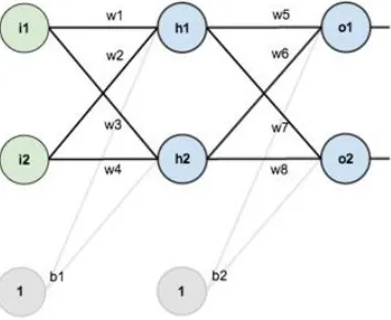
Fig. 1. Architecture of Neural Network with one hidden layer

The most common used of Neural Networks are Multilayer Perception (MLP) that

being combined with Backpropagation Learning. This configuration already proved be useful to minimize error and maximize time series forecasting accuracy. An example of work by Yohannes et al. (2015) which used this approach to forecast state minimum wage on Malang City based on inflation rate obtained error rate only 0.0728. Study that conducted by Anifa et al. (2015) to predict rice demand by using Back- propagation Neural Network resulted 94,36% accuracy, while research by Vamsidhar et al. (2010) which build rainfall forecasting model in India produces accuracy of 94,28%. Another work by Huda et.al. (2015) proof that Backpropagation Neural Network also useful to detect malware attack on Android.

3. Methodology

We will use Artificial Neural Network Algorithm with one hidden layer and two bias node to forecast the rainfall. The architecture of this method can be seen on figure 2.

(4)

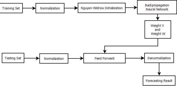
The methodology of this research consist on two categories : training networks and forecasting and the process can be seen at Fig. 3.

Fig. 3. Rainfall Forecasting Process

From training dataset, we will get the weight V and weight W. “Weight V” is a weight from input layer to hidden layer while Weight “W” symbolize the weight from hidden layer to output layer. Both of the weight will be used as parameters on feedforward phase.

The data that we will use is 360 days historical rainfall datasets from four areas in Batu Regency, Indonesia : Junggo, Pujon, Ngujung, and Tinjomulyo, and those data will be normalized into range [0.1; 0.9] by equation (1)

𝑥′_{= (0.8 ×} 𝑥−𝑚𝑖𝑛𝑣𝑎𝑙𝑢𝑒

𝑚𝑎𝑥_{𝑣𝑎𝑙𝑢𝑒}−𝑚𝑖𝑛_{𝑣𝑎𝑙𝑢𝑒}) + 0.1 (1)

Where:

x = data

x’ = normalized data

minvalue = minimum value of the data maxvalue maxvalue = maximum value of the data

Yohannes (et al. 2015)

The initial wight V from input layer to hidden layer is being initialized using Ngu- yen-Widrow Algorithm. The steps to implement Nguyen-Widrow Algorithm are :

• Determine the factor using the formula (2)

𝛽 = 0.7𝑝1 𝑛⁄ ₍₂₎

(5)

= the scalar factor

n = number of input neurons p = number of hidden neurons

• Initialize Vij using random value between [-0,5; 0,5]

• Measure the ||Vij|| using formula (3)

` ‖𝑉𝑖𝑗‖ = √∑𝑝_𝑛=1(𝑉𝑖𝑗)2 (3)

• Update to weight using formula (4)

𝑣𝑖𝑗 =𝛽×𝑣𝑖𝑗(𝑜𝑙𝑑)_{‖𝑣𝑖𝑗‖} (4)

• Make bias from input layer to hidden layer ranged between [-β, β]

This research uses classical one-hidden-layer neural network architecture. The ideal number of neurons in hidden layer must fullfill equation (5). (Heaton 2005).

𝑁ℎ𝑖𝑑𝑑𝑒𝑛 ≤2₃× 𝑁𝑖𝑛𝑝𝑢𝑡 + 𝑁𝑜𝑢𝑡𝑝𝑢𝑡 (5)

And since we use 4 neurons in input layer, based on equation (5) our hidden layer must consist neurons between 1, 2, or 3 neurons.

3.1 Feedforward Phase

There is three phases on Backpropagation Neural Network. The first one is feedforward, backpropgation and lastly update weight.(Brownlee 2011).

After weight initialization using Nguyen-Widrow algorithm that was being de- scribed on equation (4). We must calculate all output that become input on hidden layer by implement the following equation :

𝑍𝑖𝑛𝑗= 𝑏𝑖𝑎𝑠1 + ∑𝑛𝑖=1𝑋𝑖𝑉𝑖𝑗 (6)

Where :

Zinj = activation element

𝑏𝑖𝑎𝑠1 = bias between input and hidden layer on index j xi = input value on index

𝑉𝑖𝑗 = weight between input and hidden layer

After that we calculate the value of hidden layer based on equation (6) and Sig- moid activate function by using the following formula :

𝑍𝑗 =_1+𝑒_−𝑧1 _𝑖𝑛𝑗 (7)

Where :

(6)

The signal that come out from hidden layer (y ink)is being calculated by :

𝑌𝑖𝑛𝑘= 𝑏𝑖𝑎𝑠2𝑘+ ∑𝑚𝑖=1𝑋𝑖𝑉𝑗𝑘 (8)

Where :

𝑏𝑖𝑎𝑠2𝑘 = bias between hidden layer and output layer on index k

Xi = input value on index i

𝑉𝑗

𝑘

= weight between hidden layer and output layer

And finally we get output value by follow the equation (9) below :

𝑌𝑘 =_1+𝑒1_𝑦_𝑖𝑛𝑘 (9)

After the output we will get error by :

𝑒𝑟𝑟𝑜𝑟 = 𝑡 − 𝑌𝑘 (10)

where :

t = the desired output

yk = the calculated output on current iteration

By the error on equation (10) we may calculate MSE

𝑀𝑆𝐸 =∑ 𝑒𝑟𝑟𝑜𝑟_𝑛 2 (11)

Where n is number of neurons on input layer.

3.2 Backpropagation Phase

While the number of iteration didn’t exceed the iteration limit and the MSE didn’t touch the desired target error, the backpropagation will continue. On this process we will get value by :

𝛿𝑘 = 𝑡𝑘− 𝑦𝑘 𝑓′(𝑦𝑖𝑛𝑘) = (𝑡𝑘− 𝑦𝑘)𝑦𝑘(1 − 𝑦𝑘) (11)

The δk value will be used to compute weight change (ΔW)

𝑏𝑖𝑎𝑠2𝑘 = 𝛼 × 𝛿𝑘 (12)

And also bias2 value change

The output layer will send back signal to hidden layer that calculated as :

𝛿𝑖𝑛𝑗= ∑𝑝𝑘=1𝛿𝑘× 𝑊𝑗𝑘 (13)

For every unit in hidden layer we calculate a value named 𝛿1𝑗 to repair weight

(7)

𝛿1𝑗= 𝛿𝑖𝑛𝑗× 𝑓′(𝑍𝑖𝑛𝑗) (14)

And then we update weight V and bias1.

∆𝑉𝑖𝑗 = 𝛼(𝛿𝑗𝑥𝑗) (15)

∆𝑏𝑖𝑎𝑠1𝑗= 𝛼 × 𝛿𝑗 (16)

3.3 Update Weight Phase

For output layer we update the weight W and bias2

𝑊𝑗𝑘 = 𝑊𝑗𝑘+ ∆𝑊𝑗𝑘 (17)

𝑏𝑖𝑎𝑠2𝑘 = 𝑏𝑖𝑎𝑠2𝑘+ ∆𝑏𝑖𝑎𝑠2𝑘 (18)

For input layer we update the weight V and bias1

𝑉𝑗𝑘 = 𝑉𝑗𝑘+ ∆𝑉𝑗𝑘 (19)

𝑏𝑖𝑎𝑠1𝑘 = 𝑏𝑖𝑎𝑠1𝑘+ ∆𝑏𝑖𝑎𝑠1𝑘 (20)

4. Result and Discussion

By using dataset consists of 4 historical input data which the example can be seen on Table 1. We will conduct three test. First based on iteration, second based on number of neurons in hidden layer and the last will be conducted based on learning rates.

Table 1. Historical Data Example

z(t-1) z(t-2) z(t-17) z(t-34) z(t)

0 0 0 0 2,4

2,4 0 0 0 5,3

5,3 2,4 0 0 5,364

5,364 5,3 0 0 0

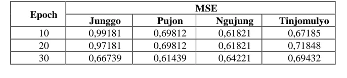
Firstly we will looking for optimum epoch or iteration number. By using iteration number from 10 until 100 with interval 10 in every test we will get result as Table 2 and its graphical interpretation on figure 4.

Table 2. Result of Epoch Test

Epoch MSE

Junggo Pujon Ngujung Tinjomulyo

10 0,99181 0,69812 0,61821 0,67185

20 0,97181 0,69812 0,61821 0,71848

(8)

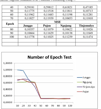
40 0,59181 0,59812 0,61821 0,47185

50 0,11775 0,11518 0,11811 0,10713

60 0,11962 0,11683 0,11198 0,11281

70 0,11827 0,11939 0,10653 0,11810

Epoch MSE

80 0,10357 0,11079 0,10622 0,11026

90 0,10664 0,11629 0,10138 0,11849

100 0,11778 0,11025 0,11239 0,11474

Fig. 4. MSE Graph of Epoch Test

By epoch 50, the MSE is reached minimum number and have no significant change among the four areas, so epoch 50 will be used on next test : the hidden layer test. By using maximum epoch 50 and number of neurons vary between 1 until 3 we will get result as shown in table 3.

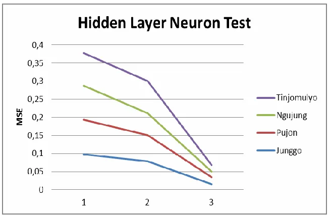
Table 3. Result of Number of Neurons in Hidden Layer Test

Number of Neu-

rons

MSE

1 0,0972131 0,09622143 0,09412294 0,09045184

2 0,07792347 0,07273976 0,06037331 0,08865956

(9)

Fig. 5. MSE Graph of Hidden Layer Test

By looking on table 2 and figure 3, we know that 3 neurons on hidden layer resulted better MSE than 1 neuron or 2 neurons on hidden layer. Therefore on next test, the learning rate test, the maximum epoch 50 and 3 neurons hidden layer will be applied.

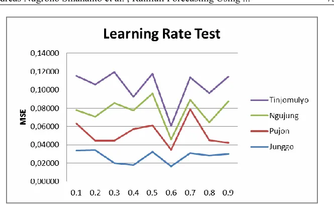
On the last test, we will conduct test of learning rate. We will test the learning rate with range between [0.1;0.9]. The result can be seen in Table 4 and Figure 4.

Table 4. Result of Learning Rate Test

Learning rate MAPE

Junggo Pujon Ngujung Tinjomu

lyo

0.1 0,03385 0,02973 0,01430 0,03778

0.2 0,03436 0,01005 0,02644 0,03535

0.3 0,02005 0,02456 0,04119 0,03376

0.4 0,01807 0,03933 0,02023 0,01493

0.5 0,03262 0,02890 0,03439 0,02161

0.6 0,01663 0,01793 0,01143 0,01467

0.7 0,03114 0,04757 0,01039 0,02468

0.8 0,02815 0,01686 0,01934 0,03196

(10)

Fig. 6. MSE Graph of Learning Rate Test

The learning rate MSE result is varied but the best learning rate is 0,8 because it has the lowest MSE set among all MSE set. We can conclude that with maximum epoch 50 iterations, hidden layer consist of 3 neurons and learning rate 0,6 we will get lowest MSE Set {0,02815; 0,01686; 0,01934; 0,03196}.

5. Conclusion

The Rainfall Forecast using Neural Network Backpropagation with Nguyen- Widrow Weight Initialization have best MSE Set 0,02815 for Junggo Area, 0,01686 for Pujon Area, 0,01934 for Ngujung Area and 0,03196 for Tinjomulyo Area on learning rate 0,6 and maximum epoch 50. Future research may implement additional method like Hybrid NN-GA to get more ideal weight and get lower MSE.

References

1.Anifa, I.A., Regasari, R., Marji: Peramalan Permintaan Beras Menggunakan Backpropaga- tion Dengan Inisialisasi Bobot Nguyen-Widrow. Universitas Brawijaya, Malang (2015). 2.Buono, A., Kurniawan, A., Komputer, D.I.: Peramalan Awal Musim Hujan Menggunakan

Jaringan Syaraf Tiruan Backpropagation Levenberg-Marquardt. 2012, 15–16 (2012).

3.Hashim, R., Roy, C., Motamedi, S., Gocic, M., Lee, S.C., Cheng, S.: Selection of meteoro- logical parameters affecting rainfall estimation using neuro-fuzzy computing methodology. Atmos. Res. 171, 21–30 (2015).

4.Heaton, J.: Introduction to Neural Network for Java. Heaton Research, Inc, St. Louis (2005). 5.Huda, F. Al, Mahmudy, W.F., Tolle, H.: Android Malware Detection Using Backpropaga-

tion Neural Network. TELKOMNIKA. 4, (2015).

6.Hung, N.Q., Babel, M.S., Weesakul, S., Tripathi, N.K.: An artificial neural network model for rainfall forecasting in Bangkok, Thailand. Hydrol. Earth Syst. Sci. 13, 1413–1425 (2008).

7.Iriany, A., Mahmudy, W.F., Sulistyono, A.D., Nisak, S.C.: GSTAR-SUR Model for Rainfall Forecasting in Tengger Region , East Java. 1st Int. Conf. Pure Appl. Res. Univ. Muham- madiyah Malang, 21-22 August. 1–8 (2015).

(11)

Technique. Int. J. Eng. Technol. 2, 397–400 (2010).

9.Luk, K.C., Ball, J.E., Sharma, A.: A study of optimal model lag and spatial inputs to artificial neural network for rainfall forecasting. J. Hydrol. 227, 56–65 (2000).

10.Mazur, M.: A Step by Step Backpropagation Example, http://mattmazur.com.

11.Nasseri, M., Asghari, K., Abedini, M.J.: Optimized scenario for rainfall forecasting using genetic algorithm coupled with artificial neural network. Expert Syst. Appl. 35, 1415–1421 (2008).

12.Oxford Dictionaries: Concise Oxford English Dictionary. Oxford University Press, Oxford- shire, UK (2009).

13.Sedki, A., Ouazar, D., El Mazoudi, E.: Evolving neural network using real coded genetic algorithm for daily rainfall-runoff forecasting. Expert Syst. Appl. 36, 4523–4527 (2009). 14.Sumi, S.M., Zaman, M.F., Hirose, H.: A rainfall forecasting method using machine learning

models and its application to the Fukuoka city case. Int. J. Appl. Math. Comput. Sci. 22, 841–854 (2012).

15.Vamsidhar, E., Varma, K., Rao, P., Satapati, R.: Prediction of rainfall using backpropagation neural network model. Int. J. Comput. Sci. Eng. 2, 1119–1121 (2010).

16.Wahyuni, I., Mahmudy, W.F., Iriany, A.: Rainfall Prediction in Tengger Region-Indonesia Using Tsukamoto Fuzzy Inference System. 1th Int. Conf. Inf. Technol. Inf. Syst. Electr. Eng. 1–11 (2016).