Environmental Resources Research
Vol. 7, No. 2, 2019
GUASNR
Impacts of combining meteorological and hydrometric data on the
accuracy of streamflow modeling
M. Motamednia1*, A. Nohegar2, A. Malekian3, M. SaberiAnari4, K. Karimi Zarchi5
1Ph.D. of Watershed Management Science and Engineering, Hormozgan University, BandarAbbas, Iran 2Professor of Learning, faculty of environment, University of Tehran, Karaj, Iran
3Associate Professor, Department of Rehabilitation of Arid and Mountainous Regions, Faculty of Natural
Resources, University of Tehran, Karaj, Iran
4Instructor of Technical and Vocational University, Yazd, Iran 5The head of Natural Resources, Bafgh District, Yazd, Iran
Received: February 2019 ; Accepted: December 2019
Abstract
Proper modeling of rainfall-runoff is essential for water quantity and quality management. However, comprehensive evaluation of soft computing techniques for rainfall-runoff modeling in developing countries is still lacking. Towards this end, in the present study two new soft computing techniques of genetic programming (GP) and M5 model tree were formulated for daily streamflow prediction. Firstly, the daily meteorological and hygrometric data including rainfall, temperature, evapotranspiration, relative humidity and discharge were collected for the years 1970 - 2012 throughout Amameh Watershed in Tehran, Iran. Secondly, the input variables were determined using cross-correlation and then 62 different scenarios were developed. Thirdly, the data were standardized in the range of zero to one. Finally, performance of the scenarios was assessed using the mean square error (MSE), root mean square error (RMSE) and mean absolute error (MAE). Totally, 80 and 20 percent of instances were used for training and testing, respectively. The results showed that the scenario number 54 was the best using both GP and M5 model tree techniques. However, GP showed much better performance than M5 model tree with MSE, RMSE, and MAE values of 0.001, 0.031 and 0.009 for training and 0.001, 0.032 and 0.009 for testing, respectively. The scenario 54 had eight inputs including rainfall, discharge, and delay for two days, temperature, evapotranspiration and relative humidity.
Keywords: Genetic programming, Model development, M5 model tree, Scenario analysis, Streamflow prediction1
Introduction
Understanding the governing properties of watershed hydrology under different
conditions is a challenging issue
throughout the globe (Huo et al., 2012; Danandeh Mehr et al., 2013; Moatamednia et al., 2015; Ghorbani et al., 2018).
Numerous factors including climate
condition, vegetation cover, soil
infiltration, and land use affect the relationship of hydrological process and
particularly rainfall-runoff processes
(Keshtegar et al., 2018; Rezaie-Balf et al., 2019). To optimally design and operate
water resources structures or to
appropriately plan structures use and maintenance we need to have detailed
information on rainfall-runoff
relationships in a particular time interval or period (Huo et al., 2012; Danandeh Mehr et al., 2013; Moatamednia et al., 2015; Rezaie-Balf and Kisi, 2017). The
increasing development trend in
computational intelligence field has led to appearance and development of computer
and technology-based rainfall-runoff
models (Solaimani, 2009; Huo et al., 2012; Chandwani, et al., 2015; Liu et al., 2017; Najafzadeh et al., 2018; Lu et al., 2018). In this field, rainfall-runoff models could be very helpful for flood control measures, drought management and water supply allocation. On the other hands,
basic information for river flow
forecasting is needed to provide solutions to a wide range of problems related to the design and operation of river systems. The availability of rainfall records and other meteorological data, which can be used to obtain streamflow data, initiated the
practice of rainfall-runoff modeling
(Behzad et al., 2009). In addition, it is well documented that the rainfall-runoff models have important role in water resource management planning, irrigation and water supply. Different models with various
degrees of complexity have been
developed (Dooge, 1977; Harun et al., 2002; Bhattacharya and Solomatine, 2005; Solaimani, 2009; Besaw et al., 2010; Fernando et al., 2011; Abrahart et al.,
2012; Motamednia et al., 2015;
Najafzadeh et al., 2016; Liu et al., 2017;
Rezaie-Balf and Kisi, 2017; Keshtegar et al., 2018; Rezaie-Balf et al., 2019).
Hydrologists are often confronted with problems of prediction and estimation of runoff, precipitation, water stages, and so on (Harun et al., 2002; Danandeh Mehr et al., 2013; Motamednia et al., 2015). System theoretic models do not consider
the physical characteristics of the
parameters; while they illustrate the data from input to output using transferred functions. Where the interactions among
the variables are complex, the
conventional mathematical techniques in the form of regression equations can’t provide a perfect representation. As functional relationship of rainfall-runoff can be extremely complex (Fernando et al., 2011), today, the soft computing tools
offer a simplified approach over
conventional hard computing in dealing with these nature based phenomena (Chandwani et al., 2015; Danandeh Mehr,
2018). Specifically, for streamflow
prediction, due to the lack of precise knowledge and the complexity of the effective factors, different models have been developed (Danandeh Mehr, 2013; Rezaie-Balf and Kisi, 2017; Rezaie-Balf et al., 2017; Keshtegar et al., 2018). Genetic programming (GP) as a clear and effective method can be used for estimation of water based data (Danandeh Mehr, 2014; Talebi et al., 2017). GP is a self-parameterizing method that build models without any user tuning (Sreekanth and Datta, 2011; Danandeh Mehr et al., 2013; Danandeh Mehr et al., 2014). A GP model is a member of the evolutionary algorithm family, which are based upon the concept of natural section and genetic evolution (Koza, 1992; Solomatine and Xue, 2004; Guven, 2009; Gorbani et al., 2010; Wang et al., 2014; Danandeh Mehr, 2018).
Genetic algorithm (GA) that was
Crossover operator in GP is applied to change the sub-tree from the parents to reproduce the children by means of mating selection policy instead of exchanging bit
strings as in GA (Wang et al., 2009). This
method works with a number of solution sets collectively known as a population rather than a single solution at any time, therefore the possibility of getting trapped in a local optimum is avoided. However, GP is different from traditional GA. in that it typically operates on parse tree instead of bit string. A parse tree is built up from a terminal set (the input variables in the
problem and randomly generated
constants, i.e. empirical model
coefficients) and a function set, hence the basic operators are used to form the GP model. The next is user-defined and can not only include algebraic operators such as {+, -, *, /, exp., sin} but also take the form of logical rules, making use of operators such as {IF, OR, AND} (Selle and Muttil, 2011).
Ghorbani et al. (2010) reported the high performance of GP in comparison with neural networks (ANN) and neuro-fuzzy (FIS) methods of flood routing of Kizilirmak River, Turkey. Ajmera and Goyal (2012) also investigated modeling of the stage–discharge in Peachtree Creek in Atlanta using ANN and M5 model tree and then the results were compared with discharge from current and traditional methods. Their results showed that, M5 model performed better than ANN. Danandeh Mehr (2013) used wavelet-ANN (Wwavelet-ANN) and linear GP (LGP) to predict river flow on a monthly scale. The GP, WANN and three-layer perceptron neural network techniques based on the
statistical evaluation showed good
performance. Additionally, an explicit LGP model constructed by only basic arithmetic functions including one month-lagged records of both target and upstream stations revealed the best prediction model for the studied river. Sattari et al. (2013) surveyed the potential of Multi-Layer Perceptron (MLP) with back propagation algorithm and M5 model tree based regression approaches to model monthly
reference evapotranspiration using
climatic data of an area around Ankara, Turkey. The results revealed that the M5 model tree, could predict river flow better than the support vector machine (SVM). It is also concluded that a simple linear relationships using M5 model tree requires less computational time. Meshgi et al. (2015) used GP for streamflow modeling in different land uses of Kent Ridge Watershed, southern part of Singapore. Al-Juboori and Guven (2016) worked on
GEP-based monthly streamflow
forecasting model for perennial rivers in Hurman River in Turkey as well as Diyalah and Lesser Zab Rivers in Iraq. They divided monthly flow data into 12 intervals because of the number of months in a year. The result showed the importance of seasonality effect in the selection of potential predictors which is the major pattern in the intermittent streamflow series. Keshtegar et al. (2018)
compared four heuristic regression
techniques such as Kriging method vs. RSM, multivariate adaptive regression spline (MARS) and M5 model tree in Adana and Antakya stations located in Eastern Mediterranean Region of Turkey. Their results showed that models M5 model tree produce inaccurate results for both maximum error and minimum agreement compared to other models. Finally, the periodic Kriging models performed superior to the periodic MARS, RSM and M5Tree models. Rezaie-Balf et al. (2019) M5 model tree (M5Tree) and MARS models to forecast river flow. They developed models using two different meteorological stations Kordkheyl in Iran and Hongcheon in South Korea. Results showed that EEMD-MARS model was an efficient and robust tool to forecast one and multi-day-ahead like two, three, and
four-day-ahead river flow. The GP model
is very similar to GA, in which each chromosome in initial population is a potential solution for a given problem. However, chromosomes in GP are represented by tree-shaped structure of a computer program that contains nodes of functions and terminals with connecting
branches (Danandeh Mehr, 2018).
completed in three steps. (1) An initial population is generated randomly for parse tree. (2) Any member of the mentioned population is considered using the fitness function for selecting better parse trees for production of new population (Gorbani et al., 2010; Wang et al., 2014). The root mean square error (RMSE) is used to meet the goal of this step, (3). In every generation, below stages are followed for population selection:
(a) One of the operators such as crossover, mutation is selected, (b)
Appropriate number of available
population is then chosen, (c) The selected operators are used to produce offspring, (d) These children are entered in a new
population, and (f) Models are evaluated by different fitting criteria. (4) The third step is repeated until the maximum
number of generations is reached
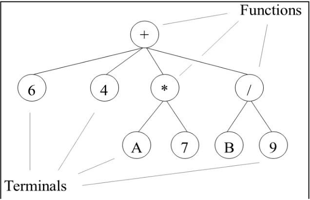
(Sreekanth and Datta, 2011; Danandeh Mehr et al., 2013). As shown in Figure 1, in GP modeling, there are functions and terminals chosen randomly from the user defined sets to form a computer model in a tree-like structure with a root node and branches extending from each function and ending in a leaf or a terminal. In many cases, in GP leaves are the inputs to the program (Koza, 1992; Babovic and Keijzer, 2000; Al-Juboori and Guven, 2016; Danandeh Mehr, 2018).
Figure 1. GP parse tree representing function (+ 6 4 (* A7) (/B9)
The M5 tree models are introduced as
new soft computing method and
generalizing the concepts of regression trees, which have constant values at their leaves (Witten and Frank, 2005; Sattari et al., 2013; Al-Juboori and Guven, 2016). M5 model tree is very capable and efficient. Today, the M5 model tree are used in various fields of hydrology and water resources, particularly in matters of classification and prediction. The M5 model trees are analogous to piece-wise linear functions (and hence nonlinear). The M5 model tree is a binary decision tree having linear regression functions at leaf nodes, which can predict continuous
al., 2018). The formula to compute the standard deviation reduction (SDR) is as follows.
(1)
SDR=sd(T)- sd(Ti)
T Ti
(2) ( ) = 1( −1 ( ) )
Where T represents a set of examples
that reach the node, Ti represents the
subset of examples that have the ith outcome of the potential set, N is the number of data and sd represents the standard deviation. Because of the splitting process, child nodes have less standard deviation as compared to parent node and are thus more pure (Quinlan, 1992). After examining all the possible splits, M5 chooses the one that maximizes the expected error reduction. This division often produces a large tree-like structure that may cause over fitting. To counter the problem of over fitting, the tree must be pruned back, for example by replacing a sub tree with a leaf.
Thus, the second stage in the design of the model tree involves pruning the overgrown tree and replacing the sub trees with linear regression functions (Etemad-Shahidi and Bonakdar, 2009; Sattari et al.,
2013; Rezaie-Balf et al., 2017; Keshtegar et al., 2018; Rezaie-Balf et al., 2019). For this, the parameter space is split into subspaces and in each a linear regression model is built.
The aim of this study was to forecast river flow using two famous methods viz. GP and M5 model tree in Amameh Watershed, Iran.
Materials and Methods Study area and data
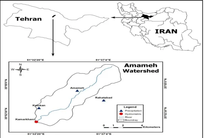
The Amameh Watershed with an area of
37.2 km2, located in 35º 51´ 50´´
N-latitude and 51º 32´ 27´´E-longitude is one of the sub-watersheds of the Jajroud Watershed in the southern part of central
Alborz, Iran (Figure 2). The average
annual temperature and rainfall are 12 °C and 350 mm, respectively. The watershed elevation ranges from 1900 to 3868 m above sea level (Nourani et al., 2009). The specific topographic features of the Amameh Watershed, the meteorological stations availability and data accessibility were the main reasons why we selected this watershed as a case study. In the present study, the daily meteorological and hydrometric data were recorded in Amameh and Kamarkhani stations located at the central and the outlet of the watershed, respectively (Figure 2).
The meteorological and hydrometric variables were used to calculate the daily streamflow for the time period 1970-1971 to 2011-2012 (42 years). Meteorological and hydrometric parameters, namely rainfall (P), mean air temperature (T), relative humidity (Rh), evapotranspiration (ET) and discharge (Q) were considered as inputs of rainfall-runoff modeling. In the training period of both GP and M5 model tree approaches, 80 % of inputs (i.e., 1970-1971 to 2003-2004; 10944 data points for 34 years) were used. The remaining 20% of inputs (2004-2005 to 2011-2012; 2920 data points for eight
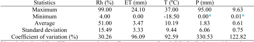
years) were used for testing of models and scenarios. Table 1 provides the statistical properties of the various meteorological and hydrometric parameters used in this study.
The data standardization was also made in order to make the data dimensionless and confine them within a certain range before entering the inputs data into training and testing steps. So, to assimilate and integrate the data, the values were normalized in the range of zero to one (Sattari et al., 2013; Danandehr Mehr et al., 2014; Motamednia et al., 2015; Danandeh Mehr, 2018).
Table 1. Statistical properties of used data for rainfall-runoff modeling of Amameh WatershedQ (m3/s)
P (mm)
C)
0
T ( ET (mm) Rh (%)
Statistics
9.63 95.00
37.00 24.10 99.00 Maximum
0.01*
0.00*
-18.50 0.00 4.00
Minimum
0.61 1.83
10.19
3.47
51.00
Average
0.75 6.06
9.44
3.33
15.49
Standard deviation
122.82 330.53 92.59 96.09 30.26 Coefficient of variation (%)
Rh=relative humidity, ET=evapotranspiration, T=temperature, P=rainfall, Q=discharge, *the value of rainfall is zero but the value of discharge is 0.01 because of baseflow and interflow
One of the most important steps in the model development process is the choice of significant input variables. Although, there is no clear cut theory and rules for that but usually solutions such as cross-autocorrelation and partial cross-autocorrelation analysis of data are used (Srinivasulu and Jain, 2006; Wu et al., 2009; Huo et al., 2012; Motamednia et al., 2015; Rezaie-Balf et al., 2017). These methods are used to reduce inputs number of variables. Cross-correlation analysis between the target streamflow Q(t) with itself and different lag time series of P, ET, Rh were performed to get the important factors for
streamflow estimation. The
cross-autocorrelation analysis between different inputs and their lags were also used (Huo
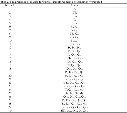
et al. 2012; Danandeh Mehr et al., 2014; Danandeh Mehr, 2018). According to the results of 62 scenarios and variables used as inputs with one to six time lags, inputs were selected for this study. Table 2 shows the study scenarios.
Table 2. The proposed scenarios for rainfall-runoff modeling of Amameh Watershed Inputs Scenario t P 1 t ET 2 t h R 3 t T 4 1 -t Q 5 1 -t , P t P 6 1 -t , Q t P 7 1 -t , Q t ET 8 1 -t , Q t h R 9 1 -t ,Q t T 10 2 -t , Q 1 -t Q 11 2 -t , P 1 -t , P t P 12 1 -t , Q 1 -t , P t P 13 2 -t , Q 1 -t , Q t P 14 2 -t , Q 1 -t , Q t ET 15 2 -t , Q 1 -t , Q t h R 16 2 -t , Q 1 -t ,Q t T 17 3 -t , Q 2 -t , Q 1 -t Q 18 1 -t , Q 2 -t , P 1 -t , P t P 19 2 -t , Q 1 -t , Q 1 -t , P t P 20 3 -t , Q 2 -t , Q 1 -t , Q t P 21 3 -t , Q 2 -t , Q 1 -t , Q t ET 22 3 -t , Q 2 -t , Q 1 -t , Q t h R 23 3 -t , Q 2 -t , Q 1 -t ,Q t T 24 t h , R t , ET t , T t P 25 4 -t , Q 3 -t , Q 2 -t , Q 1 -t Q 26 2 -t , Q 1 -t , Q 2 -t , P 1 -t , P t P 27 3 -t , Q 2 -t , Q 1 -t , Q 1 -t , P t P 28 4 -t , Q 3 -t , Q 2 -t , Q 1 -t , Q t P 29 4 -t ,Q 3 -t , Q 2 -t , Q 1 -t , Q t ET 30
Qt= represents the normalized daily discharge at the present time, Rht= represents the normalized daily
relative humidity at the present time, ETt= represents the normalized daily evapotranspiration at the
present time, Pt= represents the normalized daily rainfall humidity at the present time, Tt= represents
the normalized daily temperature at the present time, the indices t-1 to t-6 respectively refer to 1-day and 6-day lags and so on.
Efficiency criteria
The ability of models and scenarios to estimate daily discharge in Amameh Watershed was considered by applying the evaluation criteria. There are many performance criteria which have been used widely all over the world for rainfall-runoff relationship (Legates and McCabe, 1999; Dawson and Wilby, 2001; Huo et al., 2012; Moatamednia et al., 2015; Danandeh, 2018). The performance of all models in this article was evaluated by using a three statistical performance evaluation measures. These performance
criteria included mean-square error
(MSE), root-mean-square error (RMSE)
and mean absolute error (MAE)
(Srinivasulu and Jain, 2006; Danandeh et
al., 2013; Lu et al., 2018; Rezaie-Balf et al., 2019). RMSE measured the goodness of fit for high streamflow. In addition, it provided information about the predictive capabilities of the scenario. The error is the amount by which the value implied by the estimator differs from the target or quantity to be estimated (Danandeh Mehr et al., 2014). The above statistical parameters can be calculated using the following expressions (equations number 3 to 5).
where QO, Qe and N are measured and
estimated values and number of data,
respectively.
Table 2. Continued. The proposed scenarios for rainfall-runoff modeling of Amameh Watershed
Inputs Scenarios 4 -t ,Q 3 -t , Q 2 -t , Q 1 -t , Q t Rh 31 4 -t ,Q 3 -t , Q 2 -t , Q 1 -t ,Q t T 32 1 -t , Q t , Rh t , ET t , T t P 33 5 -t , Q 4 -t , Q 3 -t , Q 2 -t , Q 1 -t Q 34 3 -t , Q 2 -t , Q 1 -t , Q 2 -t , P 1 -t , P t P 35 4 -t , Q 3 -t , Q 2 -t , Q 1 -t , Q 1 -t , P t P 36 5 -t , Q 4 -t , Q 3 -t , Q 2 -t , Q 1 -t , Q t P 37 5 -t , Q 4 -t ,Q 3 -t , Q 2 -t , Q 1 -t , Q t ET 38 5 -t , Q 4 -t ,Q 3 -t , Q 2 -t , Q 1 -t Q , t Rh 39 5 -t , Q 4 -t ,Q 3 -t , Q 2 -t , Q 1 -t ,Q t T 40 t , Rh t , ET t , T 2 -t , P 1 -t , P t P 41 2 -t , Q 1 -t , Q t , Rh t , ET t , T t P 42 6 -t , Q 5 -t , Q 4 -t , Q 3 -t , Q 2 -t , Q 1 -t Q 43 4 -t ,Q 3 -t , Q 2 -t , Q 1 -t , Q 2 -t , P 1 -t , P t P 44 5 -t ,Q 4 -t ,Q 3 -t , Q 2 -t , Q 1 -t , Q 1 -t , P t P 45 6 -t , Q 5 -t , Q 4 -t , Q 3 -t , Q 2 -t , Q 1 -t , Q t P 46 6 -t ,Q 5 -t , Q 4 -t ,Q 3 -t , Q 2 -t , Q 1 -t , Q t ET 47 6 -t ,Q 5 -t , Q 4 -t ,Q 3 -t , Q 2 -t , Q 1 -t , Q t Rh 48 6 -t ,Q 5 -t , Q 4 -t ,Q 3 -t , Q 2 -t , Q 1 -t ,Q t T 49 1 -t , Q t , Rh t , ET t , T 2 -t , P 1 -t , P t P 50 3 -t , Q 2 -t , Q 1 -t , Q t , Rh t , ET t , T t P 51 5 -t ,Q 4 -t ,Q 3 -t , Q 2 -t , Q 1 -t , Q 2 -t , P 1 -t , P t P 52 6 -t , Q 5 -t ,Q 4 -t ,Q 3 -t , Q 2 -t , Q 1 -t , Q 1 -t , P t P 53 2 -t , Q 1 -t , Q t , Rh t
, Tt, ET
2 -t , P 1 -t , P t P 54 4 -t , Q 3 -t , Q 2 -t , Q 1 -t
, Tt, ETt, Rht, Q
t P 55 6 -t , Q 5 -t ,Q 4 -t ,Q 3 -t , Q 2 -t , Q 1 -t , Q 2 -t , P 1 -t , P t P 56 3 -t , Q 2 -t , Q 1 -t Q , t , Rh t , ET t , T 2 -t , P 1 -t , P t P 57 5 -t , Q 4 -t , Q 3 -t , Q 2 -t , Q 1 -t , Q t , Rh t , ET t , T t P 58 4 -t , Q 3 -t , Q 2 -t , Q 1 -t , Q t , Rh t , ET t , T 2 -t , P 1 -t , P t P 59 6 -t , Q 5 -t , Q 4 -t , Q 3 -t , Q 2 -t , Q 1 -t , Q t , RH t , ET t , T t P 60 5 -t , Q 4 -t , Q 3 -t , Q 2 -t , Q 1 -t , Q t , Rh t , ET t , T 2 -t , P 1 -t , P t P 61 6 -t , Q 5 -t , Q 4 -t , Q 3 -t , Q 2 -t , Q 1 -t , Q t , Rh t , ET t , T 2 -t , P 1 -t , P t P 62
Qt= represents the normalized daily discharge at the present time, Rht= represents the normalized daily relative
humidity at the present time, ETt= represents the normalized daily evapotranspiration at the present time, Pt=
represents the normalized daily rainfall humidity at the present time, Tt= represents the normalized daily
temperature at the present time, the indices t-1 to t-6 respectively refer to 1-day and 6-day lags and so on.
Table 3. Best parameter for GP model
Value Parameter
300
Initial population (Program)
Sum Linking function 0.044 Mutation rate 0.01 Inversion rate 0.30 One-point recombination rate
0.30 Two-point recombination rate
0.10 Gene recombination rate
0.10 Gene transposition rate
1000 Maximum generation
Results and Discussion
As already mentioned, 62 scenarios (see Table 2) were considered for rainfall-runoff modeling of Amameh Watershed using GP and M5 model tree. The best values for various parameters in GP were
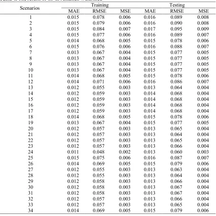
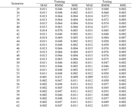
Table 4. The results of GP in Amameh Watershed Testing Training Scenarios MSE RMSE MAE MSE RMSE MAE 0.008 0.089 0.016 0.006 0.078 0.015 1 0.008 0.090 0.016 0.006 0.079 0.015 2 0.009 0.095 0.017 0.007 0.084 0.015 3 0.007 0.089 0.016 0.006 0.077 0.015 4 0.006 0.078 0.015 0.005 0.068 0.014 5 0.007 0.088 0.016 0.006 0.076 0.015 6 0.005 0.077 0.015 0.004 0.067 0.013 7 0.005 0.077 0.015 0.004 0.067 0.013 8 0.005 0.077 0.015 0.004 0.067 0.013 9 0.005 0.077 0.015 0.004 0.067 0.013 10 0.006 0.078 0.015 0.005 0.068 0.014 11 0.007 0.086 0.016 0.006 0.071 0.014 12 0.004 0.064 0.013 0.003 0.055 0.012 13 0.004 0.068 0.014 0.003 0.059 0.012 14 0.004 0.068 0.014 0.003 0.059 0.012 15 0.004 0.068 0.014 0.003 0.059 0.012 16 0.004 0.068 0.014 0.003 0.059 0.012 17 0.006 0.078 0.015 0.005 0.068 0.014 18 0.005 0.077 0.015 0.004 0.067 0.013 19 0.004 0.065 0.013 0.003 0.057 0.012 20 0.004 0.064 0.013 0.003 0.057 0.012 21 0.004 0.065 0.013 0.003 0.057 0.012 22 0.004 0.066 0.013 0.003 0.057 0.012 23 0.003 0.060 0.013 0.002 0.048 0.011 24 0.007 0.087 0.016 0.006 0.075 0.015 25 0.006 0.079 0.015 0.005 0.069 0.014 26 0.004 0.063 0.013 0.003 0.055 0.012 27 0.004 0.064 0.013 0.003 0.055 0.012 28 0.004 0.066 0.013 0.003 0.058 0.012 29 0.004 0.067 0.013 0.003 0.058 0.012 30 0.004 0.067 0.013 0.003 0.058 0.012 31 0.004 0.066 0.013 0.003 0.057 0.012 32 0.004 0.065 0.013 0.003 0.057 0.012 33 0.006 0.079 0.015 0.005 0.069 0.014 34
As can be seen from the Tables 4 and 5 in the training period, the GP method achieved the best MSE, RMSE, and MAE evaluation criteria of 0.001, 0.031, and 0.0.009, for scenario 54. Whilst the M5 method provided the best results with the least error, namely 0.057, 0.197 and 0.039, respectively for MSE, RMSE, and MAE for model 54. It can be observed from the testing period results, both GP and M5 methods have high MSE, RMSE and MAE errors in this period, namely 0.009, 0.032 and 0.001 for GP and 0.085, 0.255 and 0.065 for M5 model respectively.
Here we developed three models. The first model contained only meteorological inputs, the second model consisted of hydrometric and the third model used both
meteorological and hydrometric variables as inputs. According to error analysis of the test set model, in which we only used meteorological variable, we had higher errors than the one with hydrometric variable as input. This finding showed that
antecedent discharge of Amameh
Watershed had more effect on the results. Out of these parameters, relative humidity, evapotranspiration, rainfall and temperature had the most errors, respectively. Therefore
the least and the most effective
for M5 model tree were 0.620, 0.760 and 0.578 for training and 0.594, 0.744 and
0.553 for testing, respectively.
Table 4. Continued. The results of GP in Amameh Watershed testing
Testing Training Scenarios MSE RMSE MAE MSE RMSE MAE 0.002 0.048 0.011 0.002 0.046 0.011 35 0.003 0.060 0.013 0.002 0.048 0.011 36 0.005 0.072 0.014 0.004 0.064 0.013 37 0.005 0.072 0.014 0.004 0.064 0.013 38 0.005 0.074 0.014 0.004 0.064 0.013 39 0.005 0.071 0.014 0.004 0.063 0.013 40 0.007 0.085 0.015 0.005 0.070 0.014 41 0.002 0.048 0.011 0.002 0.046 0.011 42 0.007 0.084 0.015 0.005 0.069 0.014 43 0.003 0.058 0.012 0.002 0.048 0.011 44 0.003 0.058 0.012 0.002 0.048 0.011 45 0.005 0.076 0.015 0.004 0.066 0.013 46 0.005 0.076 0.015 0.004 0.066 0.013 47 0.005 0.076 0.015 0.004 0.066 0.013 48 0.005 0.075 0.015 0.004 0.065 0.013 49 0.002 0.047 0.011 0.002 0.046 0.011 50 0.002 0.046 0.011 0.002 0.046 0.011 51 0.003 0.057 0.012 0.002 0.048 0.011 52 0.003 0.058 0.012 0.002 0.048 0.011 53 0.001 0.032 0.009 0.009 0.031 0.001 54 0.002 0.050 0.012 0.011 0.047 0.002 55 0.003 0.057 0.012 0.011 0.048 0.002 56 0.002 0.045 0.010 0.010 0.045 0.002 57 0.003 0.055 0.012 0.011 0.047 0.002 58 0.002 0.048 0.011 0.011 0.046 0.002 59 0.003 0.057 0.012 0.011 0.048 0.002 60 0.002 0.049 0.011 0.011 0.047 0.002 61 0.003 0.055 0.012 0.011 0.047 0.002 62
The results furthermore showed that more than one variable as input affected runoff so that the combinations of meteorological and hydrometric variables were necessary. According to the results in Tables 4 and 5, the best model was number 54 in which we used the
concurrent rainfall, one and two
antecedent rainfall, the concurrent
temperature and one and two antecedent runoff, the current evapotranspiration and
relative humidity. To prevent
overgrowing, the maximum size of the program was restricted (Brameier and Banzhaf, 2001; Gorbani et al., 2010; Danandeh Mehr, 2018). The maximum generation was 1000 and the function sets were defined by modeler based on two sets of mathematical functions. The first set was the software default consisting of 11 functions such as sin, cos, tang and
cotg and the other was four basic mathematical operations {+, -, * and /} and power function. According to the results, the basic mathematical operations plus power were better than those of software default. The results showed that the rainfall-runoff relationship is complex and non-linear, and its estimation using these functions caused accuracy reduction (Danandeh Mehr, 2018). The GP model due to its high efficiency enables estimation of non-linear relationship with the basic mathematical operations. These findings were consistent with those of other researchers (Khu et al., 2001; Whigham and Crapper, 2001; Liong et al.,
2002; Jayawardena et al., 2005;
Table 5. The results of M5 in Amameh Watershed Testing Training Scenarios MSE RMSE MAE MSE RMSE MAE 0.538 0.733 0.576 0.567 0.753 0.606 1 0.546 0.739 0.588 0.572 0.756 0.612 2 0.553 0.744 0.594 0.578 0.760 0.620 3 0.530 0.728 0.566 0.550 0.742 0.592 4 0.146 0.382 0.140 0.125 0.354 0.124 5 0.524 0.724 0.558 0.535 0.731 0.573 6 0.108 0.329 0.110 0.081 0.285 0.100 7 0.109 0.330 0.110 0.084 0.290 0.100 8 0.112 0.335 0.110 0.100 0.316 0.110 9 0.108 0.329 0.110 0.081 0.285 0.100 10 0.124 0.352 0.122 0.110 0.332 0.110 11 0.495 0.704 0.514 0.412 0.642 0.472 12 0.102 0.319 0.110 0.069 0.263 0.093 13 0.104 0.322 0.110 0.071 0.266 0.096 14 0.104 0.322 0.110 0.071 0.266 0.096 15 0.104 0.322 0.110 0.071 0.266 0.096 16 0.103 0.321 0.110 0.071 0.266 0.096 17 0.127 0.356 0.126 0.110 0.332 0.110 18 0.107 0.327 0.110 0.080 0.283 0.100 19 0.102 0.319 0.110 0.069 0.263 0.093 20 0.102 0.319 0.110 0.069 0.263 0.093 21 0.102 0.319 0.110 0.069 0.263 0.093 22 0.103 0.321 0.110 0.070 0.265 0.095 23 0.100 0.316 0.110 0.068 0.261 0.091 24 0.504 0.710 0.520 0.484 0.696 0.506 25 0.151 0.389 0.140 0.132 0.363 0.130 26 0.100 0.316 0.110 0.068 0.261 0.091 27 0.102 0.319 0.110 0.069 0.263 0.093 28 0.103 0.321 0.110 0.070 0.265 0.095 29 0.103 0.321 0.110 0.070 0.265 0.095 30 0.103 0.321 0.110 0.070 0.265 0.095 31 0.103 0.321 0.110 0.070 0.265 0.095 32 0.102 0.319 0.110 0.069 0.263 0.093 33 0.170 0.412 0.152 0.140 0.374 0.134 34
Figure 3. Observed and predicted flows based on genetic programming (GP) during training
period for Amameh Watershed 0 2 4 6 8 10 1 9 7 0 -7 1 1 9 7 1 -7 2 1 9 7 3 -7 4 1 9 7 4 -7 5 1 9 7 6 -7 7 1 9 7 8 -7 9 1 9 7 9 -8 0 1 9 8 3 -8 4 1 9 8 5 -8 6 1 9 8 5 -8 7 1 9 8 5 -8 9 1 9 9 0 -9 1 1 9 9 1 -9 2 1 9 9 3 -9 4 1 9 9 5 -9 6 1 9 9 6 -9 7 1 9 9 8 -9 9 2 0 0 1 -2 0 0 2 2 0 0 3 -2 0 0 4 Time (Daily) St re a m fl o w ( m 3 /s )
Table 5. Continued. The results of M5 in Amameh watershed Testing Training Scenarios MSE RMSE MAE MSE RMSE MAE 0.097 0.311 0.110 0.064 0.253 0.083 35 0.100 0.316 0.110 0.068 0.261 0.091 36 0.104 0.322 0.110 0.072 0.268 0.098 37 0.105 0.324 0.110 0.072 0.268 0.098 38 0.105 0.324 0.110 0.074 0.272 0.100 39 0.104 0.322 0.110 0.071 0.266 0.096 40 0.484 0.696 0.506 0.402 0.634 0.464 41 0.097 0.311 0.110 0.065 0.255 0.085 42 0.175 0.418 0.158 0.148 0.385 0.140 43 0.100 0.316 0.110 0.068 0.261 0.091 44 0.100 0.316 0.110 0.068 0.261 0.091 45 0.105 0.324 0.110 0.075 0.274 0.100 46 0.106 0.326 0.110 0.078 0.279 0.100 47 0.106 0.326 0.110 0.079 0.281 0.100 48 0.105 0.324 0.110 0.075 0.274 0.100 49 0.097 0.311 0.110 0.064 0.253 0.083 50 0.097 0.311 0.110 0.063 0.251 0.081 51 0.099 0.315 0.110 0.067 0.259 0.089 52 0.100 0.316 0.110 0.068 0.261 0.091 53 0.065 0.255 0.085 0.039 0.197 0.057 54 0.098 0.313 0.110 0.066 0.257 0.087 55 0.100 0.316 0.110 0.067 0.259 0.089 56 0.096 0.310 0.110 0.063 0.251 0.081 57 0.099 0.315 0.110 0.066 0.257 0.087 58 0.097 0.311 0.110 0.065 0.255 0.085 59 0.099 0.315 0.110 0.067 0.259 0.089 60 0.097 0.311 0.110 0.065 0.255 0.085 61 0.099 0.315 0.110 0.066 0.257 0.087 62
Figure 4. Observed and predicted flows based on genetic programming (GP) during testing
period for Amameh Watershed
0 2 4 6 8 2 0 0 4 -2 0 0 5 2 0 0 4 -2 0 0 5 2 0 0 5 -2 0 0 6 2 0 0 5 -2 0 0 6 2 0 0 6 -2 0 0 7 2 0 0 6 -2 0 0 7 2 0 0 7 -2 0 0 8 2 0 0 8 -2 0 0 9 2 0 0 8 -2 0 0 9 2 0 0 9 -2 0 1 0 2 0 0 9 -2 0 1 0 2 0 1 0 -2 0 1 1 2 0 1 1 -2 0 1 2 2 0 1 1 -2 0 1 2 Time (Daily) S tr ea m fl o w ( m 3 /s )
Table 6. Relationship between variables in model number 54 provided by M5 model tree
Row Rules
1 If Qt-1 <= 0.59 Qt-2 > 0.16 Qt-1 > 0.32, Then Qt =0.003 * Pt - 0.02*Pt-1- 0.03*Pt-2 + 0.001* Rht +1.05*Qt-1-0.12*Qt-2 - 0.02 [1526/24.315%]
2 If Qt-1<=0.59 Qt-2<=0.17 Qt-1 <=0.12 Qt-1>0.09, Then Qt=0.0001*Pt-0.05*Pt-1–0.004*P
t-2+0.05*Tt-0.001*ETt+0.01*Rht+0.02*Qt-1+0.01*Qt-2+0.12[1359/4.415%]
3 If Qt-1<=0.59 Qt-1<=0.18 Rht<=51.5, Then Qt=0.0001*Pt-0.004*Pt-1-0.003*Pt-2+0.08*Tt -0.001ETt +0.001*Rht+0.92*Qt-1+0.012*Qt-2+0.009 [1636/4.382%]
4 If Qt-1<=0.59 Qt-1> 0.18Qt-1<=0.23, Then Qt=0.004*Pt-0.001*Pt-1–0.003*Pt-2+0.05*Tt– 0.004*ETt +0.003*Rht+0.66*Qt-1+0.13*Qt-2+0.034 [1016/7.214%]
5 If Qt-1 <= 0.60 Qt-1 > 0.2 Pt <= 0.75, Then Qt = 0.0001 * Pt – 0.006 * Pt-1 - 0.001 * Pt-2 + 0.004*Tt - 0.002*ETt+0.0001*Rht+0.81*Qt-1+0.10*Qt-2+0.03 [980/5.342%]
6 If Qt-1>1.08 Qt-1 <=2.24 Qt-1 <=1.60 Pt-1 <=1.65, Then Qt=0.013*Pt-0.007*Pt-1-0.004*P
t-2+0.004*Tt-0.0002*ETt+0.001*Rht+0.88*Qt-1+0.02*Qt-2+0.14 [814/29.142%]
7 If Qt-1>1.08 Qt-1<=2.30 Qt-1> 1.60, Then Qt=0.013*Pt-0.007*Pt-1-0.0002*Pt-2 +0.002*Tt+0.0001*Rht+0.63*Qt-1+0.23*Qt-2+0.24 [716/40.251%]
8 If Qt-1 <=1.08 Qt-2<=0.31 Qt-1<=0.16 Pt<=0.85, Then Qt=0.001*Pt+0.0001*Pt-1–0.0004*P
t-2+0.0001*Tt-0.0002*ETt+0.0001*Rht+0.94*Qt-1+0.012*Qt-2+0.01 [435/3.573%]
9 If Qt-1 <= 1.07 Qt-2 > 0.305 Rht <= 51.5 Qt-1 > 0.77, Then Qt=0.0003*Pt+ 0.0001*Pt-1 -0.001*Pt-2-0.003*Tt-0.0004*ETt+0.0001*Rht+0.93*Qt-1-0.09*Qt-2+ 0.173 [435/11.755%]
10 If Qt-1 > 1.075 Qt-1 > 1.95, Then Qt=0.0001*Pt -0.006*Pt-1-0.008*Pt-2+0.0001*Tt +0.008* Rht+0.442*Qt-1+0.12*Qt-2+ 0.811 [411/82.488%]
11 If Qt-2<=0.305, Then Qt=0.004*Pt+0.002*Pt-1-0.003*Pt-2+0.002*Tt-0.001*ETt +0.0001*Rht+0.498*Qt-1+0.2354* Qt-2 +0.0392 [554/31.238%]
12 If Qt-1<=0.99 Rht >51.5Qt-1>0.655, Then Qt=0.004*Pt-0.0002*Pt-1+0.009*Tt-0.025*ETt +0.0001*Rht+1.11*Qt-1+0.025* Qt-2-0.084 [378/44.009%]
13 If Qt-1>0.88 Pt-2<=7.5, Then Qt=0.008*Pt+0.001*Pt-1-0.0007*Pt-2+0.002*Tt -0.003*ETt+0.0002*Rht+0.56*Qt-1+ 0.0782 *Qt-2+0.45 [219/79.17%]
14 If Rht<=51.5 Qt-1<=0.68, Then Qt=0.001*Pt-0.0002*Pt-2+0.001*Tt-0.001*ETt +0.0002*Rht+0.99*Qt-1- 0.034*Qt-2-0.002 [129/19.56%]
15 If Pt-1<=4.75 Rht<=51.5, Then Qt=0.002*Pt-0.001*Pt-2-0.003*Tt+0.0003*Rht+0.679*Qt-1 + 0.104 * Qt-2+0.20 [139/19.388%]
16 If Tt <= 3.15, Then Qt=0.003*Pt+0.004*Tt-0.01*ETt+0.001*Rht+0.63*Qt-1+ 0.13*Qt-2 +0.069 [108/17.38%]
17 Qt =0.044* Pt + 0.02 * Rht+1.140*Qt-2 - .47 [89/65.448%]
Figure 5. Observed and predicted flows based on M5 model tree during training period for
Amameh Watershed
0 2 4 6 8 10
1
9
7
0
-7
1
1
9
7
1
-7
2
1
9
7
3
-7
4
1
9
7
4
-7
5
1
9
7
6
-7
7
1
9
7
8
-7
9
1
9
7
9
-8
0
1
9
8
3
-8
4
1
9
8
5
-8
6
1
9
8
5
-8
7
1
9
8
5
-8
9
1
9
9
0
-9
1
1
9
9
1
-9
2
1
9
9
3
-9
4
1
9
9
5
-9
6
1
9
9
6
-9
7
1
9
9
8
-9
9
2
0
0
1
-2
0
0
2
2
0
0
3
-2
0
0
4
Time (Daily)
S
tr
ea
m
fl
o
w
(
m
3 /s
)
Figure 6. Predicted and observed flow during testing period by M5 for Amameh Watershed
According to Table 6, 17 rules suggested by M5 model tree could solve this problem. Several advantages such as user friendliness, fast training process, understandable results and simple and linear equations could be noted for this model. It is important to mention that although the equations governing the M5
model were not really physically
interpretable, but they allowed the modelers to quickly check the predicted
streamflow as reported before by
Solomatine, and Dulal (2003).
Figures 3 to 6 show that although GP method could simulate and predict streamflow with low errors, but both methods of GP and M5 underestimate the Amameh Watershed streamflow, and this is especially so for M5 method in training period. We showed that flow peaks of the
study datasets often led to poor
performances. Furthermore, high accuracy of prediction could not be achieved by this model (Wu and Chen, 2005; Ni et al., 2010; Danandeh Mehr et al., 2014; Dnandeh Mehr, 2018). In the case of Hao et al. (2006), the data used for prediction were much smoother and this could have had something to do with their good forecasting.
The final mathematical relationship
obtained using GP for Amameh
Watershed is expressed as follows:
) 6 ( Qt=(Qt-2/Qt-1)((RHtQt-1 *0.92Pt))+(Qt-1
-(0.02Pt-1)0.06))+0.089Tt+0.089Pt-2
-ETt)
The results showed that the GP model had good simulation and prediction due to low errors during training and testing periods, respectively. This finding verified the results of Selle and Muttil (2011) who studied the GP in southeastern Australia. It is believed that GP could be used to get insight into the dominant events of hydrological cycles, practically.
Conclusion
The experimental Amameh Watershed in Tehran Province, Iran was subjected to
rainfall-runoff modeling using two
approaches of GP and M5 model tree under 62 different scenarios. The results showed better performance of GP in almost all scenarios for daily streamflow prediction. It was also found that GP had appropriate potential for solving complex and nonlinear hydrological modeling problems. The results indicated that the relative humidity (Rh) had the least
sensitivity in streamflow prediction
among other meteorological variables i.e., rainfall (P), mean air temperature (T), and evapotranspiration (ET). Furthermore, the performances of all developed scenarios were assessed using standard statistical 0
2 4 6 8
2
0
0
4
-2
0
0
5
2
0
0
4
-2
0
0
5
2
0
0
5
-2
0
0
6
2
0
0
5
-2
0
0
6
2
0
0
6
-2
0
0
7
2
0
0
6
-2
0
0
7
2
0
0
7
-2
0
0
8
2
0
0
8
-2
0
0
9
2
0
0
8
-2
0
0
9
2
0
0
9
-2
0
1
0
2
0
0
9
-2
0
1
0
2
0
1
0
-2
0
1
1
2
0
1
1
-2
0
1
2
2
0
1
1
-2
0
1
2
Time (Daily)
S
tr
ea
m
fl
o
w
(
m
3
/s
performance evaluation measures such as MSE, RMSE and MAE. However, we recommend error analysis for varying
ranges of flow such as low, medium and high streamflow.
References
Abrahart, R.J., Anctil, F., Coulibaly, P., Dawson, C.W., Mount, N.J., See, L.M., Shamseldin, A.Y., Solomatine, D.P., Toth, E., and Wilby, R.L. 2012. Two decades of anarchy? Emerging themes and outstanding challenges for neural network modelling of surface hydrology. Progress in Physial Geography, 36 (4), 480–513.
Ajmera, T.K., Goyal, M.K. 2012. Development of stage–discharge rating curve using model tree and neural networks: An application to Peachtree Creek in Atlanta, Expert Systems with Applications, 39, 5702–5710.
Al-Juboori A.M., and Guven A. 2016. A stepwise model to predict monthly streamflow. Journal of Hydrology, 543, 283-292.
Babovic, V., and Keijzer, M. 2000.Geneticprogrammingasamodelinductionengine. Journal of Hydroinform, 2, 35–60.
Behzad, M., Asghari, K., Eazi, M., and Palhang, M. 2009. Generalization performance of support vector machines and neural networks runoff modelling. Expert System with Applications, 36, 7624-7629.
Besaw, L.E., Rizzo, D.M., Bierman, P.R., and Hackett, W.R. 2010. Advances in ungauged streamflow prediction using artificial neural networks. Journal Hydrology, 386, 27–37. Brameier, M., and Banzhaf, W. 2001. A comparison of linear genetic programming and neural
networks in medical data mining. IEEE Trans. Evolutionary Computation, 5, 17–26. Bhattacharya, B., and Solomatine, D.P. 2005. Neural networks and M5 model trees in modelling water level–discharge relationship. Neurocomputing, 63, 381-396.
Chandwani, V., Vyas, S.K., Agrawal, V., and Sharma, G. 2015. Soft computing approach for
rainfall-runoff modelling: A review, International Conference on Water Resources, Costal
and Ocean Engineering (ICWRCOE 2015), Aquatic Procedia, 4, 1054-1061.
Danandeh Mehr, A., Kahya, E., and Olyaie, E. 2013. Streamflow prediction using linear genetic programming in comparison with a neuro-wavelet technique, Journal of Hydrology, 505, 240–249.
Danandeh Mehr, A., Kahya, E., and Yerdelen, C. 2014. Linear genetic programming application for successive-station monthly streamflow prediction, Journal of Computers and Geosciences, 70, 63–72.
Dawson, C.W., and Wilby, R.L. 2001. Hydrological modelling using artificial neural network, Progress in Physical Geography, 25(1), 80–108.
Dooge, J.C.I. 1977. Problems and methods of rainfall-runoff modelling. In: Ciriani, T.A., U. Maione and J.R. Wallis. 2008. Mathematical Models for Surface Water Hydrology: The Workshop Held at the IBM Scientific Center, Pisa. Wiley, London, 71-108.
Etemad-Shahidi, A., and Mahjoobi, J. 2009. Comparison between M5 model tree and neural networks for prediction of significant wave height in Lake Superior, Journal of Ocean Engineering, 1175-1181.
Fernandoa, A.K., Shamseldinb, A.Y., and Abrahart, R.J. 2011. Comparison of two data-driven approaches for daily river flow forecasting, Proceedings of 19th International Congress on Modelling and Simulation, Perth, Australia, pp.1077-1083.
Ghorbani, M.A., Khatibi, R., Mehr, A.D., and Asadi, H. 2018. Chaos-based multigene genetic programming: A new hybrid strategy for river flow forecasting. Journal of Hydrology, 562, 455-467.
Ghorbani, M.A.,Khatibi,R., Aytek, A., Makarynskyy, O., Shiri, J.,2010.Seawaterlevel forecasting using genetic programming and artificial neural networks. Computers and Geoscience. 36(5), 620–627.
Hao, Y.H., Yeh, T.C.J., Gao, Z.Q.,Wang, Y.R., and Zhao, Y. 2006. A gray system model for studying the response to climate change: the Liulin Karst springs, China. J. Hydrol. 328, 668. Harun, S., Ahmat Nor, N.I., and Kassim, M.A.H. 2002. Artificial neural network model for
rainfall-Runoff Relationship. Journal of technology, 37, 1-12.
Huo, Z., Feng, S., Kang, S., Huang, G., Wang, F., and Guo, P. 2012. Integrated neural networks for monthly river flow estimation in arid inland basin of Northwest China, Journal of Hydrology, 420–421, 159–170.
Jayawardena AW, Muttil N Fernando TMKG, 2005. Rainfall-Runoff Modelling using Genetic Programming.Pp.1841-1847. International Congress on Modelling and Simulation Society of Australia and New Zealand December 2005, New Zealand.
Keshtegar, B., Mert, C., and Kisi, O. 2018. Comparison of four heuristic regression techniques in solar radiation modeling: Kriging method vs RSM, MARS and M5 model tree, Renewable and Sustainable Energy Reviews, 81(1), 330-341.
Khu ST, Liong SY, Babovic V, Madsen H and Muttil N, 2001. Genetic programming and its application in real- time runoff forming. Journal of American Water Resource Associate, 37(2), 439-451.
Koza, J.R. 1992. Genetic Programming: On the Programming of Computers by Means of Natural Selection. MIT Press, Cambridge, MA.
Legates, D.R., and McCabe, G.J. 1999. Evaluating the use of ‘goodness-of-fit’ measures in hydrologic and hydroclimatic model validation. Water Resources Research 35, 233–41 Liong, S.Y., Gautam, T.R., Khu, S.T., Babovic, V., Keijzer, M., and Muttil N. 2002. Genetic
Programming: A new paradigm in rainfall runoff modelling. Search Results Journal of the American Water Resources Association, 38(3), 705-718.
Liu, K., Yao, C., Chen, J., Li, Z., Li, Q., and Sun, L. 2017. Comparison of three updating models for real time forecasting: a case study of flood forecasting at the middle reaches of the Huai River in East China. Stochastic Environmental Research and Risk Assessment, 31(6), 1471-1484.
Lu, X., Wang, X., Zhang, L., Zhang, T., Yang, C., Song, X., and Yang, Q. 2018. Improving forecasting accuracy of river flow using gene expression programming based on wavelet decomposition and de-noising. Hydrology Research, 49(3), 711-723
Meshgi, A., Schmitter, P., Chui, T.F.M., and Babovic, V. 2015. Development of a modular streamflow model to quantify runoff contributions from different land uses in tropical urban environments using Genetic Programming, Journal of Hydrology, 525,711–723.
Motamednia, M., Nohegar, A., Malekian, A., Asadi, H., Tavasoli, A., Safari, M., Karimi and Zarchi, K. 2015. Daily river flow forecasting in a semi-arid region using two data- driven, Desert, 20, 11-21.
Najafzadeh, M., Rezaie-Balf, M., Rashedi, E. (2016). Prediction of maximum scour depth around piers with debris accumulation using EPR, MT, and GEP models. Journal of Hydroinformatics, 18(5), 867-884
Najafzadeh, M., Rezaie-Balf, M., and Tafarojnoruz, A. 2018. Prediction of riprap stone size under overtopping flow using data-driven models. International Journal of River Basin Management, 1-8.
Ni, Q., Wang, L., Ye, R., Yang, F., and Sivakumar, M. 2010. Evolutionary modelling for streamflow forecasting with minimal datasets: a case study in the West Malian River, China. Environmental Engineering Science, 27(5), 377-385.
Nourani, V., Singh, V.P., and Delafrouz, H. 2009. Three geomorphological rainfall–runoff models based on the linear reservoir concept, Catena, 76, 206–214.
Quinlan, J.R. 1992. Learning with continuous classes. In: Adams, Sterling, editors. Proceedings of AI'92. World Scientific. p. 343-348.
Rezaie-Balf, M., Naganna, S.R., Ghaemi, A., and Deka, P.C. 2017. Wavelet coupled MARS and M5 Model Tree approaches for groundwater level forecasting. Journal of Hydrology, 553, 356-373.
Rezaie-Balf, M., Kim, S., Fallah, H., and Alaghmand, S. 2019. Daily river flow forecasting using ensemble empirical mode decomposition based heuristic regression models: Application on the perennial rivers in Iran and South Korea, Journal of Hydrology, 572, 470-485.
Sattari, M.T., Pal, M., Apaydin, H., and Ozturk, F. 2013. M5 Model Tree Application in Daily River Flow Forecasting in Sohu Stream, Turkey, Water Resources, 40 (3), 233–242.
Selle, S., and Muttil, N. 2011. Testing the structure of a hydrological model using Genetic Programming, Journal of Hydrology, 397, 1–9.
Sinivasulu, S., and Jain, A. 2006. A comparative analysis of training methods for artificial neural network rainfall-runoff models. Applied Soft Computing, 6, 295-306.
Solaimani, K. 2009. Rainfall-Runoff prediction based on artificial neural network (A case study: Jarahi Watershed). American-Eurasian Journal of Agriculture and Environment Science, 5(6), 856-865.
Solomatine, D.P., and Dulal, K.N. 2003. Model trees as an alternative to neural networks in rainfall–runoff modelling. Hydrological Sciences Journal, 48(3), 399-411.
Solomatine, D.P., and Xue, Y. 2004. M5 model trees and neural networks: application to flood forecasting in the upper reach of the Huai River in China. ASCE Journal of Hydrologic Engineering, 9(6), 491-501.
Sreekanth, J., and Datta, B. 2011. Coupled simulation-optimization model for coastal aquifer management using genetic programming-based ensemble surrogate models and multiple-realization optimization. Water Resources Research, 47(4), W04516.
Talebi, A., Mahjoobi, J., Dastorani, M.T., and Moosavi, V. 2017. Estimation of suspended sediment load using regression trees and model trees approaches (Case study: Hyderabad drainage basin in Iran). ISH Journal of Hydraulic Engineering, 23(2), 212-219.
Ustoorikar, K., and Deo, M.C. 2008. Filling up gaps in wave data with genetic programming. Marine Structures, 21, 177-195.
Wang, W.C., Chau, K.W., Cheng, Ch.T., and Qiu, L. 2009. A Comparison of performance of several artificial intelligence methods for forecasting monthly discharge time series, Journal of Hydrology, 374 (3-4), 294-306.
Wang, Y., Guo, S., Chen, H., and Zhou, Y. 2014. Comparative study of monthly inflow prediction methods for the Three Gorges Reservoir. Stoch. Environ. Res. Risk Assess. 28, 555–570.
Whigham, P.A., and Crapper, P.F. 2001. Modelling Rainfall-Runoff Relationships using Genetic Programming, Mathematic land Computer Modelling, 33, 707-721.
Witten, I.H., and Frank, E. 2005. Data Mining: Practical Machine Learning Tools and Techniques with Java Implementations. Morgan Kaufmann: San Francisco. 2005.
Wu, C.L., Chau, K.W., and Li, Y.S. 2009. Methods to improve neural network performance in daily flows prediction, Journal of Hydrology, 372 (1-4) 80-93.
Wu, W.Y., and Chen, S.P. 2005. A prediction method using the grey model GMC (1, n) combined with the grey relational analysis: a case study on Internet access population forecast. Applied Mathematics and Computation, 1, 1-10.