Distributed Inference for Linear Support Vector Machine

Distributed Inference for Linear Support Vector Machine

Xiaozhou Wang [email protected]

School of Mathematical Sciences

Shanghai Jiao Tong University, Shanghai, 200240, China

Zhuoyi Yang [email protected]

Stern School of Business

New York University, New York, NY 10012, USA

Xi Chen [email protected]

Stern School of Business

New York University, New York, NY 10012, USA

Weidong Liu [email protected]

School of Mathematical Sciences and MoE Key Lab of Artificial Intelligence Shanghai Jiao Tong University, Shanghai, 200240, China

Editor:Qiang Liu

Abstract

The growing size of modern data brings many new challenges to existing statistical inference methodologies and theories, and calls for the development of distributed inferen-tial approaches. This paper studies distributed inference for linear support vector machine (SVM) for the binary classification task. Despite a vast literature on SVM, much less is known about the inferential properties of SVM, especially in a distributed setting. In this paper, we propose a multi-round distributed linear-type (MDL) estimator for conducting inference for linear SVM. The proposed estimator is computationally efficient. In partic-ular, it only requires an initial SVM estimator and then successively refines the estimator by solving simple weighted least squares problem. Theoretically, we establish the Bahadur representation of the estimator. Based on the representation, the asymptotic normality is further derived, which shows that the MDL estimator achieves the optimal statistical efficiency, i.e., the same efficiency as the classical linear SVM applying to the entire data set in a single machine setup. Moreover, our asymptotic result avoids the condition on the number of machines or data batches, which is commonly assumed in distributed estimation literature, and allows the case of diverging dimension. We provide simulation studies to demonstrate the performance of the proposed MDL estimator.

Keywords: Linear support vector machine, distributed inference, Bahadur representa-tion, asymptotic theory

1. Introduction

The development of modern technology has enabled data collection of unprecedented size. Very large-scale data sets, such as collections of images, text, transactional data, sensor network data, are becoming prevailing, with examples ranging from digitalized books and newspapers, to collections of images on Instagram, to data generated by large-scale net-works of sensing devices or mobile robots. The scale of these data brings new challenges to

c

traditional statistical estimation and inference methods, particularly in terms of memory restriction and computation time. For example, a large text corpus easily exceeds the mem-ory limitation and thus cannot be loaded into memmem-ory all at once. In a sensor network, the data are collected by each sensor in a distributed manner. It will incur an excessively high communication cost if we transfer all the data into a center for processing, and moreover, the center might not have enough memory to store all the data collected from different sensors. In addition to memory constraints, these large-scale data sets also pose challenges in computation. It will be computationally very expensive to directly apply an off-the-shelf optimization solver for computing the maximum likelihood estimator (or empirical risk min-imizer) on the entire data set. These challenges call for new statistical inference approaches that are able to not only handle large-scale data sets efficiently, but also achieve the same statistical efficiency as classical approaches.

In this paper, we study the problem of distributed inference for linear support vector machine (SVM). SVM, introduced by Cortes and Vapnik (1995), has been one of the most popular classifiers in statistical machine learning, which finds a wide range of applications in image analysis, medicine, finance, and other domains. Due to the importance of SVM, various parallel SVM algorithms have been proposed in machine learning literature; see, e.g., Graf et al. (2005); Forero et al. (2010); Zhu et al. (2008); Hsieh et al. (2014) and an overview in Wang and Zhou (2012). However, these algorithms mainly focus on addressing the computational issue for SVM, i.e., developing a parallel optimization procedure to minimize the objective function of SVM that is defined on given finite samples. In contrast, our paper aims to address the statistical inference problem, which is fundamentally different. More precisely, the task of distributed inference is to construct an estimator for the population risk minimizer in a distributed setting and to characterize its asymptotic behavior (e.g., establishing its limiting distribution).

As the size of data becomes increasingly large, distributed inference has received a lot of attentions and algorithms have been proposed for various problems (please see the related work Section 2 and references therein for more details). However, the problem of SVM possesses its own unique challenges in distributed inference. First, SVM is a classification problem that involves binary outputs {−1,1}. Thus, as compared to regression problems, the noise structure in SVM is different and more complicated, which brings new technical challenges. We will elaborate this point with more details in Remark 1. Second, the hinge loss in SVM is non-smooth. Third, instead of considering the fixed dimensionpas in many existing theories on asymptotic properties of SVM parameters (see, e.g., Lin, 1999; Zhang, 2004; Blanchard et al., 2008; Koo et al., 2008), we aim to study the diverging p case, i.e.,

p→ ∞ as the sample sizen→ ∞.

To address aforementioned challenges, we focus ourselves on the distributed inference for linear SVM, as the first step to the study of distributed inference for more general SVM.1 Our goal is three-fold:

1. The obtained estimator should achieve the same statistical efficiency as merging all the data together. That is, the distributed inference should not lose any statistical efficiency as compared to the “oracle” single machine setting.

2. We aim to avoid any condition on the number of machines (or the number of data batches). Although this condition is widely assumed in distributed inference literature (see Lian and Fan, 2017 and Section 2 for more details), removing such a condition will make the results more useful in cases when the size of the entire data set is much larger than the memory size or in applications of sensor networks with a large number of sensors.

3. The proposed algorithm should be computationally efficient.

To simultaneously achieve these three goals, we develop a multi-round distributed linear-type (MDL) estimator for linear SVM. In particular, by smoothing the hinge loss using a spe-cial kernel smoothing technique adopted from the quantile regression literature (Horowitz, 1998; Pang et al., 2012; Chen et al., 2018), we first introduce a linear-type estimator in a single machine setup. Our linear-type estimator requires a consistent initial SVM estimator that can be easily obtained by solving SVM on one local machine. Given the initial estima-tor βe₀, the linear-type estimator has a simple and explicit formula that greatly facilitates

the distributed computing. Roughly speaking, givennsamples (yi,Xi) fori= 1, . . . , n, our

linear-type estimator takes the form of “weighted least squares”:

e

β=h1

n

n

X

i=1

ui(yi,Xi,βe₀)X_iXT_i

| {z }

A1

i−1n1

n

n

X

i=1

vi(yi,Xi,βe₀)y_iX_i−w(βe₀)

| {z }

A2

o

, (1)

where the termA1is a weighted gram matrix andui(yi,Xi,βe₀)∈_Ris the weight that only

depends on the i-th data (yi,Xi) and βe₀. In the vector A₂, w(βe₀) is a fixed vector that

only depends on βe₀ and v_i(y_i,X_i,βe₀)∈Ris the weight that only depends on (y_i,X_i,βe₀).

The formula in (1) has a similar structure as weighted least squares, and thus can be easily computed in a distributed environment (noting that each term inA1 and A2 only involves

the i-th data point (yi,Xi) and there is no interaction term in Equation 1). In addition,

the linear-type estimator in (1) can be efficiently computed by solving a linear equation system (instead of computing matrix inversion explicitly), which is computationally more attractive than solving the non-smooth optimization in the original linear SVM formulation. The linear-type estimator can easily refine itself by using the βe on the left hand side

of (1) as the initial estimator. In other words, we can obtain a new linear-type estimator by recomputing the right hand side of (1) using βe as the initial estimator. By successively

refining the initial estimator for q rounds/iterations, we could obtain the final multi-round

distributed linear-type (MDL) estimatorβe (q)

. The estimatorβe (q)

not only has its advantage in terms of computation in a distributed environment, but also has describable statistical

properties. In particular, with a small number q, the estimator βe (q)

(see Theorem 1). Then the asymptotic normality follows immediately from the Bahadur representation. It is worthwhile noting that the Bahadur representation (see, e.g., Bahadur, 1966; Koenker and Bassett Jr, 1978; Chaudhuri, 1991) provides an important characteriza-tion of the asymptotic behavior of an estimator. For the original linear SVM formulacharacteriza-tion, Koo et al. (2008) first established the Bahadur representation. In this paper, we establish the Bahadur representation of our multi-round distributed linear-type estimator.

Finally, it is worthwhile noting that our algorithm is similar to a recently developed algorithm for distributed quantile regression (Chen et al., 2018), where both algorithms rely on a kernel smoothing technique and linear-type estimators. However, the technique for establishing the theoretical property for linear SVM is quite different from that for quantile regression. The difference and new technical challenges in linear SVM will be illustrated in Remark 1 (see Section 3).

The rest of the paper is organized as follows. In Section 2, we provide a brief overview of related works. Section 3 first introduces the problem setup and then describes the proposed linear-type estimator and MDL estimator for linear SVM. In Section 4, the main theoretical results are given. Section 5 provides the simulation studies to illustrate the performance of MDL estimator of SVM. Conclusions and future works are given in Section 6. We provide the proofs of our theoretical results in Appendix A.

2. Related Works

In distributed inference literature, the divide-and-conquer (DC) approach is one of the most popular approaches and has been applied to a wide range of statistical problems. In the standard DC framework, the entire data set of n i.i.d. samples is evenly split into

N batches or distributed on N local machines. Each machine computes a local estimator using them=n/N local samples. Then, the final estimator is obtained by averaging local estimators. The performance of the DC approach (or its variants) has been investigated on many statistical problems, such as density parameter estimation (Li et al., 2013), kernel ridge regression (Zhang et al., 2015), high-dimensional linear regression (Lee et al., 2017) and generalized linear models (Chen and Xie, 2014; Battey et al., 2018), semi-parametric partial linear models (Zhao et al., 2016), quantile regression (Volgushev et al., 2017; Chen et al., 2018), principal component analysis (Fan et al., 2017), one-step estimator (Huang and Huo, 2015), high-dimensional SVM (Lian and Fan, 2017),M-estimators with cubic rate (Shi et al., 2017), and some non-standard problems where rates of convergence are slower than

n1/2and limit distributions are non-Gaussian (Banerjee et al., 2018). On one hand, the DC approach enjoys low communication cost since it only requires one-shot communication (i.e., taking the average of local estimators). On the other hand, almost all the existing work on DC approaches requires a constraint on the number of machines. The main reason is that the averaging only reduces the variance but not the bias of each local estimator. To make the variance the dominating term in the final estimator constructed by taking averaging, the constraint on the number of machines is unavoidable. In particular, in the DC approach for linear SVM in Lian and Fan (2017), the number of machinesN has to satisfy the condition

In fact, to relax this constraint, several multi-round distributed methods have been recently developed (see Wang et al., 2017; Jordan et al., 2018). In particular, the key idea behind these methods is to approximate the Newton step by using the local Hessian matrix computed on a local machine. However, to compute the local Hessian matrix, their methods require the second-order differentiability on the loss function and thus are not applicable to problems involving non-smooth loss such as SVM.

The second line of the related research is the support vector machine (SVM). Since it was proposed by Cortes and Vapnik (1995), there is a large body of literature on SVM from both machine learning and statistics community. The readers might refer to the books (Cristianini and Shawe-Taylor, 2000; Sch¨olkopf and Smola, 2002; Steinwart and Christmann, 2008) for a comprehensive review of SVM. In this section, we briefly mention a few relevant works on the statistical properties of linear SVM. In particular, the Bayes risk consistency and the rate of convergence of SVM have been extensively investigated (see, e.g., Lin, 1999; Zhang, 2004; Blanchard et al., 2008; Bartlett et al., 2006). These works mainly concern the asymptotic risk. For the asymptotic properties of underlying coefficients, Koo et al. (2008) first established the Bahadur representation of linear SVM under the fixedp setting. Jiang et al. (2008) proposed interval estimators for the prediction error for general SVM. For the large p case, there are two common settings. One assumes that p grows to infinity at a slower rate than (or linear in) the sample sizenbut without any sparsity assumption. Our paper also belongs to this setup. Under this setup, Huang (2017) investigated the angle between the normal direction vectors of SVM separating hyperplane and corresponding Bayes optimal separating hyperplane under spiked population models. Another line of research considers high-dimensional SVM under a certain sparsity assumption on underlying coefficients. Under this setup, Peng et al. (2016) established the error bound in L1 norm.

Zhang et al. (2016a) and Zhang et al. (2016b) investigated the variable selection problem in linear SVM.

3. Methodology

3.1. Preliminaries

In a standard binary classification problem setting, we consider a pair of random variables {X, Y} with X ∈ X ⊆Rp and Y ∈ {−1,1}. The marginal distribution of Y is given by

P(Y = 1) =π+ and P(Y =−1) =π− where π+, π−>0 andπ++π−= 1. We assume that

the random vector X has a continuous distribution on X given Y. Let {Xi, yi}i=1,...,n be

i.i.d. samples drawn from the joint distribution of random variables {X, Y}. In the linear classification problem, a hyperplane is defined by β0+XTβ= 0 withβ= (β1, β2, ..., βp)T.

DefineXf= (1, X₁, ..., X_p)T and the coefficient vectorβe = (β₀, β₁, ..., β_p)T. For convenience

purpose we also definel(X;βe) =β₀+XTβ=fX T

e

β. In this paper we consider the standard non-separable SVM formulation, which takes the following form

fλ,n(βe) =

1

n

n

X

i=1

1−yil(Xi;βe)

++ λ

2kβk

2

2, (2)

e

β_{SVM all}= arg min

e

β∈Rp+1

Here (u)+ = max(u,0) is the hinge loss, λ > 0 is the regularization parameter and k · k2

denotes the Euclidean norm of a vector. We note that we do not penalize the first coordinate

β0 and thus the regularization is only imposed on β instead of βe. Throughout this paper,

for any (p+ 1)-dimensional parameter vector α_e, we will use α to denote the subvector of

e

α without the first coordinate, and only αwill appear in the regularization term. The corresponding population loss function is defined as

L(βe) =E[1−Y l(X;βe)]₊.

We denote the minimizer for the population loss by

e

β∗ = arg min

e

β∈_Rp+1

E[1−Y l(X;βe)]₊. (4)

Koo et al. (2008) proved that under some mild conditions (see Koo et al., 2008 Theorem 1,2), there exists a unique minimizer for (4) and it is nonzero (i.e., βe

∗

6

=0). We assume that these conditions hold throughout the paper. The minimizer βe

∗

of the population loss function will serve as the “true parameter” in our estimation problem and the goal is to construct an estimator and make inference ofβe

∗

. We further define some useful quantities as follows:

= 1−Y l(X,βe ∗

), and i= 1−yil(Xi,βe ∗

).

The reason why we use the notation is because it plays a similar role in the theoretical analysis as the noise term in a standard regression problem. However, as we will show in Section 3 and 4, the behavior of is quite different from the noise in a classical regression setting since it does not have a continuous density function (see Remark 1). Next, denote by δ(·) the Dirac delta function, we define

S(βe) =−_E[I{1−YfX T

e

β≥0}YfX],

D(βe) =_E[δ(1−YfX T

e

β)fXfX T

],

(5)

whereI{·}is the indicator function.

The quantities S(βe) and D(βe) can be viewed as the gradient and Hessian matrix of

L(βe) and we assume that the smallest eigenvalue of D(βe ∗

) is bounded away from 0. In fact these assumptions can be verified under some regular conditions (see Koo et al., 2008 Lemma 2, Lemma 3 and Lemma 5 for details) and are common in SVM literature (e.g., Zhang et al., 2016b Condition 2 and 6).

3.2. A Linear-type Estimator for SVM

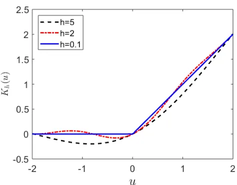
Figure 1: An example of the smoothed hinge loss functionKh with different bandwidth h.

See Section 5 for details in the construction ofH(·).

the bandwidth h →0, H(u_h) and 1_hH0(u_h) approaches the indicator function I{u≥0} and Dirac delta function δ(u) respectively, and Kh(u) approximates the hinge loss max(u,0)

(see Figure 1 for an example ofKh with different bandwidths). To motivate our linear-type

estimator, we first consider the following estimator with the non-smooth hinge loss in linear SVM replaced by its smooth approximation:

e

β_h= arg min

e

β∈Rp+1

1

n

n

X

i=1 h

1−yil(Xi;βe) i

H 1−yil(Xi;βe) h

!

+λ 2kβk

2 2

= arg min

e

β∈Rp+1

1

n

n

X

i=1

Kh(1−yil(Xi;βe)) +

λ

2kβk

2 2.

(6)

Since the objective function is differentiable and dKh(x)

dx = H(x/h) + x hH

0_{(x/h), by the}

first order condition (i.e., setting the derivative of the objective function in (6) to zero), βe_h

satisfies

1

n

n

X

i=1

(−yifX_i) "

H 1−yil(Xi;βeh) h

!

+1−yil(Xi;βeh)

h H

0 1−yil(Xi;βe_h)

h

!#

+λ

0 β_h

= 0.

We first rearrange the equation and express βe_h by

e

β_h =

"

1

n

n

X

i=1 f

XifX T

i

1

hH

0 1−yil(Xi;βe_h)

h

!#−1

×

(

1

n

n

X

i=1 yifX_i

"

H 1−yil(Xi;βeh) h

!

+1

hH

0 1−yil(Xi;βe_h)

h

!#

−λ

0 β_h

)

.

This fixed-point form formula forβe_h cannot be solved explicitly since βe_h appears on both

sides of (7). Nevertheless,βe_his not our final estimator and is mainly introduced to motivate

our estimator. The key idea is to replace βe_h on the right hand side of (7) by a consistent

initial estimatorβe₀ (e.g., βe₀ can be constructed by solving a linear SVM on a small batch

of samples). Then, we obtain the following linear-type estimator forβe ∗

:

e

β=

"

1

n

n

X

i=1 f

XifX T

i

1

hH

0 1−yil(Xi;βe₀)

h

!#−1

×

(

1

n

n

X

i=1 yifX_i

"

H 1−yil(Xi;βe0) h

!

+1

hH

0 1−yil(Xi;βe₀)

h

!#

−λ

0 β₀

)

.

(8)

Notice that (8) has a similar structure as weighted least squares (see the explanations in the paragraph below (1) in the introduction). As shown in the following section, this weighted least squares formulation can be computed efficiently in a distributed setting.

3.3. Multi-Round Distributed Linear-type (MDL) Estimator

It is important to notice that given the initial estimatorβe₀, the linear-type estimator in (8)

only involves summation of matrices and vectors computed for each individual data point. Therefore based on (8), we will construct a multi-round distributed linear-type estimator (MDL estimator) that can be efficiently implemented in a distributed setting.

First, let us assume that the total data indices {1, ..., n} are divided into N subsets {H₁, ...,H_N}with equal sizem=n/N. Denote byD_k={(Xi, yi) :i∈ Hk} the data in the

k-th local machine. In order to computeβe, for each batch of data D_k for k= 1, ..., N, we

define the following quantities

Uk=

1

n

X

i∈Hk yifX_i

"

H 1−yil(Xi;βe0) h

!

+1

hH

0 1−yil(Xi;βe₀)

h

!#

,

Vk=

1

n

X

i∈Hk

f

XifX T

i

1

hH

0 1−yil(Xi;βe₀)

h

!

.

(9)

Given βe₀, the quantities U_k,V_k can be computed independently in each machine and

only (Uk,Vk) has to be stored and transferred to the central machine. Then after receiving

(Uk,Vk) from all the machines, the central machine can aggregate the data and compute

the estimator by

e

β(1)=

N

X

k=1

Vk

!−1 _N X

k=1

Uk−λ

0 β₀

!

.

Then βe (1)

can be sent to all the machines to repeat the whole process to construct βe (2)

usingβe (1)

as the new initial estimator. The algorithm is repeatedq times for a pre-specified

q (see Equation 21 for details), and βe (q)

Algorithm 1 Multi-round distributed linear-type estimator (MDL) for SVM

Input: Samples stored in the machines {D1, ...,DN}, the number of iterations q, smooth

functionH, bandwidths{h1, ..., hq} and regularization parameter λ.

1: forg= 1, . . . , qdo 2: if g= 1then

3: Compute the initial estimator based onD1: e

β₀ = arg min

e

β∈Rp+1

1

m

X

i∈H1

1−yil(Xi;βe)

+. 4: else

5: βe₀ =βe (g−1) 6: end if

7: βe₀ is transferred to all the local machines.

8: for k= 1, . . . , N do

9: Compute (Uk,Vk) according to (9) with data in Dk using the bandwidth hg.

10: Transfer (Uk,Vk) to the central machine.

11: end for

12: The central machine computes the estimator βe (g)

by

e

β(g)=

N

X

k=1

Vk

!−1 _N X

k=1

Uk−λ

0 β₀

!

. (10)

13: end for

Output: The final MDL estimatorβe (q)

.

We notice that instead of computing matrix inversion

PN

k=1Vk

−1

in every iteration

which has a computation costO(p3), one only needs to solve a linear system in (10). Linear system has been studied in numeric optimization for several decades and many efficient algorithms have been developed, such as conjugate gradient method (Hestenes and Stiefel, 1952). We also notice that we only have to solve a single optimization problem on one local machine to compute the initial estimator. Then at each iteration, only matrix multiplication and summation needs to be computed locally which makes the algorithm computationally efficient. It is worthwhile noticing that according to Theorem 2 in Section 4, under some mild conditions, if we choose h := hg = max

λ,pp/n,(p/m)2g−2

for 1 ≤ g ≤ q, the

MDL estimatorβe (q)

achieves optimal statistical efficiency as long asq satisfies (21), which is usually a small number. Therefore, a few rounds of iterations would guarantee good performance for the MDL estimator.

For the choice of the initial estimator in the first iteration, we propose to construct it by solving the original SVM optimization (2) only on a small batch of samples (e.g., the samples on the first machine D1). The estimator βe₀ is only a crude estimator for βe

∗

optimal statistical efficiency under some regularity conditions. In particular, if we compute the initial estimator in the first round on the first batch of data, we will solve the following optimization problem

e

β₀ = arg min

e

β∈Rp+1

1

m

X

i∈H1

1−yil(Xi;βe)

+.

Then we have the following proposition from Zhang et al. (2016b).

Proposition 1 (Zhang et al. (2016b)) Under conditions (C1)-(C6) in Zhang et al. (2016b), we have

kβe₀−βe ∗

k2=OP(

p

p/m).

According to our Theorem 1, the initial estimator βe₀ needs to satisfy kβe₀ − βe ∗

k₂ =

O_P(pp/m), and therefore the estimator computed on the first machine is a valid initial estimator. On the other hand, one can always use different approaches to construct the initial estimatorβe₀ as long as it is a consistent estimator.

Remark 1 We note that although Algorithm 1 has a similar form as the DC-LEQR esti-mator for quantile regression (QR) in Chen et al. (2018), the structures of the SVM and QR problems are fundamentally different and thus the theoretical development for establishing the Bahadur representations for SVM is more challenging. To see that, let us recall the quantile regression model:

Y =Xf T

e

β∗+, (11)

where is the unobserved random noise satisfying Pr( ≤ 0|Xf) = τ and τ is known as

the quantile level. The asymptotic results of QR estimators heavily rely on the Lipschitz continuity assumption on the conditional density f(|fX) of given Xf, which has been

assumed in almost all existing literature. In the SVM problem, the quantity:= 1−YfX T

e

β∗ plays a similar role as the noise in a regression problem. However, since Y ∈ {−1,1} is binary, the conditional distribution f(|fX) becomes a two-point distribution, which no

longer has a density function. To address this challenge and derive the asymptotic behavior of SVM, we directly work on the joint distribution of and fX. As the dimension of fX

(i.e.,p+ 1) can go to infinity, we use a slicing technique by considering the one-dimensional marginal distribution offX (see Condition (C2) and proof of Theorem 1 for more details).

3.4. Communication-Efficient Implementation

In this section, we discuss a communication-efficient implementation of the proposed MDL estimator. Note that in Algorithm 1, each local machine transmits a (p+ 1)-by-(p+ 1) matrixVk to the central machine at each iteration. In fact, the communication of (p+

1)-by-(p+ 1) matrices can be avoided by using the approximate Newton method (see, e.g., Shamir et al., 2014; Wang et al., 2017; Jordan et al., 2018). Instead of transmitting the Hessian matrix Vk, we will only use the local Hessian matrix V1 computed on the first

machine. More specifically, the estimator βe (g)

in (10) essentially solves the minimization problem

arg min

e

β∈Rp+1

1 2βe

T XN

k=1

Vk

!

e

β−βe T XN

k=1

Uk−λ

0 β₀

!

The approximate Newton method uses the following iterations to solve the above minimiza-tion problem:

e

β(g,t)=βe (g,t−1)

−NVb₁

−1 XN

k=1

Vkβe (g,t−1)

−Uk

+λ

0 β₀

!

, βe (g,0)

=βe₀, (13)

as an inner iterative procedure, which approximately solves the equation (10). In (13), we let Vb₁ = V₁ in (9) with the bandwidth h =

p

p/m. The matrix NVb₁ is used to

approximate the Hessian matrix PN

k=1Vk in (12). To compute the minimizer of (13), we

note that the matrix Vb₁ only involves the data on the first machine, and thus there is

no need to communicate (p+ 1)-by-(p+ 1) matrices to compute (13). In fact, each local

machine only transmits a (p+ 1)-by-1 vector Vkβe (g,t−1)

−Uk to the central machine. We

present the entire communication-efficient implementation in Algorithm 2.

Recall that βe (g)

is the estimator defined in (10). It is easy to show that βe (g,t)

in (13)

converges toβe (g)

at a super-linear rate:

kβe (g,t)

−βe (g)

k2 ≤ I−Vb

−1 1

1

N

N

X

k=1

Vk

kβe

(g,t−1)

−βe (g)

k2,

where k · k denotes the spectral norm of a matrix. By repeatedly applying the argument, we have the following proposition, whose proof is relegated to Appendix A.3.

Proposition 2 Assume that the conditions of Theorem 1 in Section 4 hold. Suppose that

p=O(mν) for some 0< ν <1 andn=O(mA) for some A >0. We have

kβe (g,t)

−βe (g)

k₂=O_P(m−δt) (14)

for some constant δ >0, where δ and O_P(1) do not depend on t.

Proposition 2 and the convergence rate of βe (g)

(see Theorem 1) imply that the inner pro-cedure takes at most constant-valued iterations to achieve the same convergence rate as

e

β(g). Therefore the theoretical results of the MDL estimator in Algorithm 1 (see Theorem 1 and 2 in Section 4) still hold for Algorithm 2. In summary, as compared to Algorithm 1, Algorithm 2 only requires O(p) communication cost for each local machine. Therefore, Algorithm 2 is communicationally more efficient when p is large.

4. Theoretical Results

In this section, we give a Bahadur representation of the MDL estimator βe (q)

and establish its asymptotic normality result. From (8), the difference between the MDL estimator and the true coefficient can be written as

e

β−βe ∗

=D−1_n,h

An,h−λ

0 β₀

, (15)

whereAn,h=An,h(βe₀),D_n,h=D_n,h(βe₀), and for anyα_e,A_n,h(α_e) andD_n,h(α_e) are defined

Algorithm 2 Communication-efficient MDL for SVM

Input: Samples stored in the machines{D1, ...,DN}, the number of outer iterations q, the

number of inner iterationsT, smooth function H, bandwidths{h1, ..., hq} and

regular-ization parameter λ.

1: forg= 1, . . . , qdo 2: if g= 1then

3: Compute the initial estimator based onD₁:

e

β₀ = arg min

e

β∈_Rp+1 1

m

X

i∈H1

1−yil(Xi;βe)

+. 4: else

5: βe₀ =βe (g−1) 6: end if

7: Let βe (g,0)

=βe₀.

8: for t= 1, . . . , T do

9: βe

(g,t−1)

is transferred to all the local machines.

10: fork= 1, . . . , N do

11: Compute Vkβe

(g,t−1)

−Uk and transfer it to the central machine.

12: end for

13: The central machine computes βe (g,t)

by

e

β(g,t)=βe (g,t−1)

−NVb1

−1 XN

k=1

Vkβe (g,t−1)

−Uk

+λ

0 β₀

!

,

14: whereVb₁ is defined as V₁ in (9) but with the bandwidth h= p

p/m.

15: end for 16: Let βe

(g)

=βe (g,T)

.

17: end for

Output: The final MDL estimatorβe (q)

.

An,h(αe) =

1

n

n

X

i=1 yiXf_i

"

H

1−yil(Xi;αe)

h

+1−yil(Xi;βe

∗

)

h H

0

1−yil(Xi;αe)

h

#

,

Dn,h(αe) =

1

nh

n

X

i=1 f

XifX T

i H0

1−yil(Xi;αe)

h

For a good initial estimator βe₀ which is close to βe ∗

, the quantities An,h(βe₀) and

Dn,h(βe₀) are close toA_n,h(βe ∗

) andDn,h(βe ∗

). Recall thati= 1−yifX T

i βe ∗

and we have

An,h(βe ∗

) = 1

n

n

X

i=1 yiXf_i

h

Hi h

+i

hH 0i

h

i

,

Dn,h(βe ∗

) = 1

nh

n

X

i=1 f

XifX T

i H

0i

h

.

Whenhis close to zero, the termH i

h

+i

hH

0 i

h

in parenthesis ofAn,h(βe ∗

) approximates

I{i ≥ 0}. Therefore, An,h(βe ∗

) will be close to _n1 Pn

i=1yifX_iI{_i ≥ 0}. Moreover, since 1

hH

0_{(·/h) approximates Dirac delta function ash→0,D}

n,h(βe ∗

) approaches

Dn(βe ∗

) = 1

n

n

X

i=1

[δ(i)fX_ifX T

i ].

When n is large, Dn(βe ∗

) will be close to its corresponding population quantity D(βe ∗

) =

E[δ()fXXf T

] defined in (5).

According to the above argument, when βe₀ is close to βe ∗

, An,h(βe₀) and D_n,h(βe₀)

approximate _n1 Pn

i=1yifX_iI{_i ≥0} and D(βe ∗

), respectively. Therefore, by (15), we would expect βe−βe

∗

to be close to the following quantity,

D(βe ∗

)−1 1

n

n

X

i=1

yifX_iI{_i≥0} −λ

0 β∗

!

. (16)

We will see later that (16) is exactly the main term of the Bahadur representation of the estimator. Next, we formalize these statements and present the asymptotic properties of An,handDn,hin Proposition 3 and 4. The asymptotic properties of the MDL estimator will

be provided in Theorem 1. To this end, we first introduce some notations and assumptions for the theoretical result.

Recall that β∗ = (β∗₁, ..., β_p∗)T and for X = (X1, ..., Xp)T, let X−s be a (p −

1)-dimensional vector with Xs removed from X. Similar notations are used for β. Since

we assumed that βe ∗

6

= 0, without loss of generality, we assume β₁∗ 6= 0 and its absolute value is lower bounded by some constantc >0 (i.e.,|β₁∗| ≥c). Let f and g be the density functions ofX whenY = 1 andY =−1 respectively. Letf(x|X−1) be the conditional

den-sity function of X1 given (X2, ..., Xp)T and f−1(x−1) be the joint density of (X2, ..., Xp)T.

Similar notations are used forg(·).

We state some regularity conditions to facilitate theoretical development of asymptotic properties of An,h andDn,h.

(C0) There exists a unique nonzero minimizer βe ∗

for (4) with S(βe ∗

) = 0, and c ≤ λmin(D(βe

∗

))≤λmax(D(βe ∗

))≤c−1 for some constantc >0.

(C1) |β₁∗| ≥c andkβe ∗

(C2) Assume that sup_x∈R|f(x|X−1)| ≤C, supx∈R|f

0_(x|X

−1)| ≤C, supx∈R|xf

0_(x|X −1)| ≤ C, sup_x∈R|xf(x|X−1)| ≤ C, supx∈R|x

2_f(x|X

−1)| ≤ C and supx∈R|x

2_f0_(x|X −1)| ≤ Cfor some constantC >0. Also assumeR

R|x|f(x|X−1)dx <∞. Similar assumptions

are made forg(·).

(C3) Assume that p = o(nh/logn) and sup_kvk2≤1Eexp(t0|vTX|2) ≤ C for some t0 > 0

and C >0.

(C4) The smoothing function H(x) satisfies H(x) = 1 ifx ≥1 and H(x) = 0 if x ≤ −1, and also assume thatHis twice differentiable andH(2)is bounded. Moreover, assume thath=o(1).

As we discussed in Section 3.1, condition (C0) is a standard assumption which can be implied by some mild conditions (see Koo et al., 2008 (A1)-(A4)). Conditions (C1) is a mild condition on the boundness of βe

∗

. Condition (C2) is a regularity condition on the conditional density off andg, and it is satisfied by commonly used density functions, e.g., Gaussian distribution and uniform distribution. Condition (C3) is a sub-Gaussian condition on X. Condition (C4) is a smoothness condition on the smooth functionH(·) and can be easily satisfied by a properly chosenH(·) (e.g., see an example in Section 5).

Under the above conditions, we give Proposition 3 and Proposition 4 for the asymptotic

behavior of An,h and Dn,h, respectively. Recall that i = 1−yifX T

i βe ∗

and we have the following propositions. The proofs of all results in this section are relegated to Appendix A.2.

Proposition 3 Under conditions (C0)-(C4), assume that we have an initial estimator βe₀

with kβe₀−βe ∗

k₂ =O_P(an), where an is the convergence rate of the initial estimator. We

choose the bandwidth such that an=O(h), then we have

An,h(βe₀)−

1

n

n

X

i=1

yiXf_iI{_i≥0} 2

=O_P

r

phlogn

n +a

2

n+h2

!

.

Proposition 4 Suppose the same conditions in Propositions 3 hold, we have

Dn,h(βe0)−D(βe ∗

)

=OP

r

plogn

nh +an+h

!

.

According to the above propositions, with some algebraic manipulations and condition (C0), we have

e

β−βe ∗

=D(βe ∗

)−1 1

n

n

X

i=1

yifX_iI{_i≥0} −λ

0 β∗

!

+rn, (17)

with

krnk2=OP

r

p2_logn n2_h +

r

phlogn

n +a

2

n+h2

!

By appropriately choosing the bandwidth h such that it shrinks with an at the same

rate (see Theorem 1),a2_nbecomes the dominating term on the right hand side of (18). This implies that by taking one round of refinement, theL2 norm ofβe−βe

∗

improves fromO_P(an)

to O_P(a2_n) (note that kβe₀−βe ∗

k2 = OP(an), see Proposition 3). Therefore by recursively

applying the argument in (17) and setting the obtained estimator as the new initial estimator

e

β₀, the algorithm iteratively refines the estimatorβe. This gives the Bahadur representation

of our MDL estimator βe (q)

forq rounds of refinements (see Algorithm 1).

Theorem 1 Under conditions (C0)-(C4), assume that the initial estimator βe₀ satisfies

kβe₀−βe ∗

k₂ = O_P(pp/m). Also, assume p = O(m/(logn)2) and λ = O(1/logn). For a given integer q≥1, let the bandwidth in the g-th iteration be

h:=hg= max(λ,

p

p/n,(p/m)2g−2) for 1≤g≤q. Then we have

e

β(q)−βe ∗

=D(βe ∗

)−1 1

n

n

X

i=1

yifX_iI{_i ≥0} −λ

0 β∗

!

+rn, (19)

with

krnk2 =OP

r

phqlogn

n +

p

m

2q−1

+λ2

!

. (20)

It is worthwhile noting that the choice of bandwidthhgin Theorem 1 is up to a constant.

One can choose hg = C0max( p

p/n,(p/m)2g−2) for a constant C0 > 0 in practice and

Theorem 1 still holds. We omit the constantC0 for simplicity of the statement (i.e., setting C0 = 1). We notice that the algorithm is not sensitive to the choice of C0. Even with

a suboptimal constant C0, the algorithm still shows good performance with a few more

rounds of iterations (i.e., using a largerq). Please see Section 5 for a simulation study that shows the insensitivity to the scaling constant.

According to our choice ofhq, we can see that as long as the number of iterations satisfies

q≥1 + log₂

logn−logp

logm−logp

, (21)

the bandwidth ishq=

p

p/n. Then by (20), the Bahadur remainder term rn becomes

krnk2=OP((p/n)

3/4_(logn)1/2_+λ2_{). (22)}

When λ ≥ pp/n, the convergence rate βe (q)

−βe ∗

in (19) is dominated by λ. On the

other hand, ifλ=O(pp/n), then βe (q)

−βe ∗

achieves the optimal rateO_P(pp/n).

Remark 2 (The conditions on p and kβe₀−βe ∗

k₂) In this paper, we assume that the initializer is computed on the first machine with the convergence rate kβe₀ −βe

∗

of the estimator, but also provides us with a concise rate in the Bahadur remainder term (see Equation 20).

In fact, the assumption is not necessary if we assume that there is an initializerβe₀ that

satisfies kβe₀−βe ∗

k2 =OP(n

−δ_{) for some constantδ >0. Let h}

g = max(λ,

p

p/n, n−2g−1δ) and assume that conditions (C0)-(C4) hold. By the proof of Theorem 1, we have

krnk2 =OP

r

phqlogn

n +n

−2q_δ

+λ2

!

.

As long as the number of iterationsq satisfies

q≥log₂

logn−logp δlogn

, (23)

which is usually a small number in practice, we still obtain the optimal rate of the Bahadur remainder term in (22).

Remark 3 (Choice of the batch size m) The data batch size m balances the tradeoff between communication cost and computation cost. More specifically, when the batch size

mis large, the convergence rate of the initial estimator is faster. Then, the required number of iterations becomes smaller (see Equation 21), which leads to a smaller communication cost. On the other hand, for a large batch size m, the computation cost of the initial estimator is large. Moreover, the computation time of Uk and Vk on each local machine

also grows linearly in m. When the batch size m is small, the computation of the initial estimator becomes faster but it requires more iterations to achieve the same performance.

In practice, when the data is collected by multiple machines, the batch size will naturally be the storage size of each local machine. If we are allowed to specifym, we first need to make sure that m should be large enough so that the initial estimator is consistent. Moreover, since the communication is usually the bottleneck in distributed computing, it is desirable to choose m to be as large as possible to reach the capacity/memory limit of each local machine. This will provide a faster convergence rate of the initial estimator, and thus leads to a smaller number of iterations.

Remark 4 (Unbalanced batch size case) When the sample sizes on local machines are not balanced, we will choose the machine with the largest local sample size as the first machine to compute the initial estimator. This will provide us an initial estimator with faster convergence rate. As compared to the balanced case, our MDL estimator will require a smaller number of iterations to achieve the optimal statistical efficiency. It is worth noting that after the initial estimator is given, the MDL estimator in Algorithm 1 does not depend on the sample size on each local machine.

Define G(βe ∗

) =E[fXXf T

I{1−YfX T

e

β∗≥0}]. By applying the central limit theorem to (19), we have the following result on the asymptotic distribution of βe

(q)

−βe ∗

Theorem 2 Suppose that all the conditions of Theorem 1 hold with h = hg and λ =

o(n−1/2). Further, assume thatn=O(mA)for some constantA≥1,p=o(min{n1/3/(logn)2/3, mν}) for some 0< ν <1 and q satisfies (21). For any nonzero v˜ ∈_Rp+1_{, we have as n, p→ ∞,}

n1/2v˜T(βe (q)

−βe ∗

)

q

˜ vTD(βe

∗

)−1G(βe ∗

)D(βe ∗

)−1v˜

→ N(0,1).

Please see Appendix A.2 for the proofs of Theorem 1 and Theorem 2. We impose the conditions n = O(mA) and p = o(mν) for some constants A ≥ 1 and ν ∈ (0,1) in order to ensure the right hand side of (21) is bounded by a constant, which implies that we only need to perform a constant number of iterations even when n, m→ ∞.

We introduce the vector ˜v since we consider the diverging p regime and thus the di-mension of the “sandwich matrix” D(βe

∗

)−1G(βe ∗

)D(βe ∗

)−1 is growing in p. Therefore, it is notationally convenient to introduce an arbitrary vector ˜v to make the limiting vari-ance ˜vTD(βe

∗

)−1G(βe ∗

)D(βe ∗

)−1v˜ a positive real number. Also note that the conditions

p=o(n1/3/(logn)2/3) guarantees that the remainder term (22) satisfieskrnk2 =oP(n

−1/2_),

which enables the application of the central limit theorem.

It is also important to note that the asymptotic variance ˜vTD(βe ∗

)−1G(βe ∗

)D(βe ∗

)−1v˜ in Theorem 2 matches the optimal asymptotic variance ofβe_{SVM all}in (3), which is directly

computed on all samples (see Theorem 2 in Koo et al., 2008). This result shows that the

MDL estimatorβe (q)

does not lose any statistical efficiency as compared to the linear SVM in a single machine setup. By contrast, the na¨ıve divide-and-conquer approach requires the number of local machines N to satisfy the condition N ≤(n/log(p))1/3 (see Remark 1 in Lian and Fan, 2017). When this condition fails, the asymptotic normality of the estimator no longer holds. The MDL estimator removes the restriction on the number of machines but requires more communications overhead. In particular, the total communication cost for the MDL approach isO(p2N q) (orO(pN qT) for Algorithm 2), as compared to the one-shot communicationO(pN) in the na¨ıve divide-and-conquer approach. It is worth noting that, under the assumptionsn=O(mA) andp=O(mν) for some constantsA >0 and 0< ν <1 (see Proposition 2), a constant number of iterations (i.e.,qT =O(1)) is enough to achieve the optimal rate.

We note that to construct the confidence interval of ˜vTβe ∗

based on Theorem 2, we need consistent estimators of D(βe

∗

) and G(βe ∗

). Since G(βe ∗

) is defined as an expectation, it is

natural to estimate it by its empirical version Gb(βe (q)

). Moreover, by Proposition 4, we can

estimate D(βe ∗

) by Dn,h(βe (q−1)

) = N−1PN

k=1Vk. Since Dn,h(βe (q−1)

) has already been obtained in the algorithm in the last iteration, we don’t need extra computation. Given the nominal coverage probability 1−ρ0, the confidence interval for ˜vTβe

∗

is given by

˜ vTβe

(q)

±n−1/2z_ρ0/2

q

˜ vTDb(βe

(q−1)

)−1 b

G(βe (q)

)Db(βe (q−1)

)−1_{v˜, (24)}

wherezρ0/2 is the 1−ρ0/2 quantile of the standard normal distribution. For a fixed vector ˜

v, denote bσn,q = q

˜ vTDb(βe

(q−1)

)−1Gb(βe (q)

)Db(βe (q−1)

Theorem 3 (Plug-in estimation of the confidence interval) Under the conditions of Theorem 2, for any nonzero v˜∈Rp+1, we have as n, p→ ∞,

P

˜ vTβe

(q)

−n−1/2zρ0/2σbn,q ≤v˜ T

e

β∗≤v˜Tβe (q)

+n−1/2zρ0/2bσn,q

→1−ρ0.

In the proof, we first show that Gb(βe (q)

) is a consistent estimator of G(βe ∗

). The detailed proof of Theorem 3 is relegated to Appendix A.2.

Remark 5 (Kernel SVM) It is worthwhile to note that the proposed distributed algo-rithm can also be used in solving nonlinear SVM by using feature mapping approximation techniques. In the general SVM formulation, the objective function is defined as follows:

min

e

β=(β0,β)

n

X

i=1

1−yi(φ(Xi)Tβ+β0)

++ λ

2kβk

2

2, (25)

where the function φ is the feature mapping function which maps Xi to a high or even

infinite dimensional space. The functionK:Rp×Rp →Rdefined byK(x,z) =φ(x)Tφ(z) is called the kernel function associated with the feature mappingφ. With kernel mapping approximation, we construct a low dimensional feature mapping approximationψ:Rp →Rd such that ψ(x)Tψ(z) ≈φ(x)Tφ(z) =K(x,z). Then the original nonlinear SVM problem (25) can be approximated by

min

e

β∈_Rd+1

n

X

i=1

1−yi(ψ(Xi)Tβ+β0)

++ λ

2kβk

2

2. (26)

Several feature mapping approximation methods have been developed for kernels with some nice properties (see, e.g., Rahimi and Recht, 2008; Lee and Wright, 2011; Vedaldi and Zisserman, 2012), and it is also shown that the approximation error|ψ(x)Tψ(z)−K(x,z)| is small under some regularity conditions. We note that we should use a data-independent feature mapping approximation where ψ only depends on the kernel function K. This ensures that ψ can be directly computed without loading data, which enables efficient algorithm in a distributed setting. For instance, for the RBF kernel, which is defined as

KRBF(x,z) = exp −σkx−zk22

, Rahimi and Recht (2008) proposed a data-independent approximationψ as

ψ(X) =

r

2

d[cos(v T

1X+ω1), ...,cos(vTdX +ωd)]T,

wherev1, ...,vd∈Rpare i.i.d. samples from a multivariate Gaussian distributionN(0,2σI) and ω1, ..., ωd are i.i.d. samples from the uniform distribution on [0,2π].

Remark 6 (High-dimensional extension) We note that it is possible to extend the proposed MDL estimator to the high-dimensional case. In particular, with the smoothing technique used in our paper, we have the following smoothed loss function,

Ln(βe) =

1

n

n

X

i=1

Kh(1−yil(Xi;βe)) +

λ

2kβk

whereKh(u) =uH(u_h) is the smoothed hinge loss. Since the loss functionLn(βe) is

second-order differentiable, we can adopt the regularized approximate Newton method (see, e.g., Jordan et al., 2018; Wang et al., 2017). More specifically, the regularized approximate Newton method considers the following estimator,

e

β₁= arg min

e

β∈_Rp+1

{L1(βe)−βe T

(∇L1(βe₀)− ∇L_n(βe₀)) +

˜

λ

2kβk1}, (27)

where βe₀ is an initial estimator and L₁(βe) is the smoothed loss function computed using

the data on the first machine. It can be extended to an iterative algorithm by repeatedly updating the estimator using (27). However, there are two technical challenges. First, the smoothed loss function becomes non-convex. Second, it is unclear how to choose the bandwidthhsuch that it shrinks properly with the number of iterations. We leave these two technical questions and the extension to the high-dimensional case for future investigation.

5. Simulation Studies

In this section, we provide a simulation experiment to illustrate the performance of the proposed distributed SVM algorithm. The data is generated from the following model

P(Yi = 1) =p+, P(Yi =−1) =p−= 1−p+,

Xi =Yi1+i, i ∼ N(0, σ2I), i= 1,2, ..., n,

where1 is the all-one vector (1,1, ...,1)T∈Rp and the triplets (Yi,Xi,i) are drawn

inde-pendently. We set σ =√p throughout the simulation study. In order to directly compare the proposed estimator to other estimators, we follow the simulation study setting in Koo et al. (2008) and consider the optimization problem without penalty term, i.e., λ= 0. We set p+ = p− = 1₂, i.e., the data is generated from the two classes with equal probability.

Note that we can explicitly solve the true coefficient βe ∗

by the following claim whose proof is relegated to Appendix A.3.

Claim 1 The true coefficient vector isβe ∗

= 1_a(0,1, ...,1)T∈_Rp+1_{, where a is the solution}

to Ra

−∞φ1(x)xdx= 0 and φ1(x) is the p.d.f. of the distribution N(p, σ2p).

We use the integral of a kernel function as the smoothing function:

H(v) =

 



0 ifv≤ −1,

1 2+

15 16 v−

2 3v3+

1 5v5

if|v|<1,

1 ifv≥1.

The initial estimatorβe₀is computed by directly solving the convex optimization problem

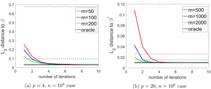
(a)p= 4,n= 104 case (b)p= 20,n= 106 case

Figure 2: L2 error of three estimators with different number of iterations q. The dashed

horizontal lines show the performance of the Na¨ıve-DC for different values of m

and the solid lines show the performance of the MDL estimators (for differentm) and the oracle estimator.

confidence intervals are constructed for ˜vT₀βe ∗

with all these three estimators, where ˜v0 =

(p+ 1)−1/21p+1 and the nominal coverage probability 1−ρ0 is set to 95%. We use (24)

to construct the confidence interval and we also use the same interval length for all the three estimators. We compare both the L2 distance between the estimator and the true

coefficientβe ∗

and the empirical coverage rate for all the three estimators.

5.1. L2 Error and Empirical Coverage Rate

We first investigate how the L2 error of our proposed estimator improves with the number

of aggregations. We consider two settings: the number of samples n = 104, dimension

p = 4, batch size m ∈ {50,100,200} and n = 106_{, p = 20, m ∈ {500,1000,2000}. We set}

the max number of iterations as 10 and plot the L2 error at each iteration. We also plot

the L2 error of Na¨ıve-DC estimator (the dashed line) and the oracle estimator (the black

line) as horizontal lines for comparison. All the results reported are the average of 1000 independent runs. From Figure 2 we can see that the error of proposed MDL estimator decreases quickly with the number of iterations. After 5 rounds of aggregations, the MDL estimator performs better than the Na¨ıve-DC approach and it almost achieves the sameL2

error as the oracle estimator.

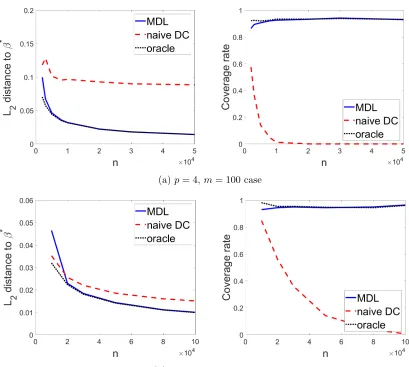
Next, we experiment on how the performance of the estimators changes with the total number of data points n while the number of data that each machine can store is fixed. We consider two settings where the machine capacity m = 100 and 1000, the number of iterations q = 10 and dimension p = 4 and 20, and we plot the L2 error and empirical

(a)p= 4, m= 100 case

(b)p= 20,m= 1000 case

Figure 3: L2 error and coverage rate of the MDL estimator with different total sample size n(the number of iterationsq = 10).

From Figure 3 we can observe that the L2 error of the oracle estimator decreases as n

increases, but the Na¨ıve-DC estimator clearly fails to converge to the true estimator which is essentially due to the fact that the bias of the Na¨ıve-DC estimator does not decrease with

n. However, the proposed MDL estimator converges to the true coefficient with almost the identical rate as the oracle estimator. We also notice that the coverage rate of the MDL estimator is quite close to that of the oracle estimator which is close to the nominal coverage probability 95%, while the coverage rate of the Na¨ıve-DC estimator quickly decreases and drops to zero whennincreases.

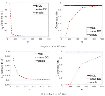
The next experiment shows how theL2 error and the coverage rate change with different

(a)p= 4,n= 105_case

(b)p= 20,n= 106 _case

Figure 4: L2 error and coverage rate of the MDL estimator with different batch sizem(the

number of iterationsq= 10).

The results are shown in Figure 4. From Figure 4 we can see that when the machine capacity gets small, theL2 error of the Na¨ıve-DC estimator increases drastically and it fails

when m ≤ 100 in the n = 105 case and m ≤ 400 in the n = 106 case. On the contrary, the MDL estimator is quite robust even when the machine capacity is small. Moreover, the empirical coverage rate for the Na¨ıve-DC estimator is small and only approaches 95% when

m is sufficiently large, while the coverage rate for the proposed MDL estimator is close to the oracle estimator which is close to the nominal coverage probability 95%.

5.2. Bias and Variance Analysis

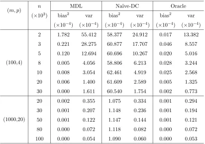
(n, p) m MDL Na¨ıve-DC Oracle

bias2 (×10−4)

var

(×10−4)

bias2 (×10−4)

var

(×10−4)

bias2 (×10−4)

var

(×10−4)

(104_,4)

100 0.004 3.906 59.329 4.457 0.000 2.275

200 0.002 2.516 10.678 2.950 0.000 2.275

500 0.005 2.459 1.393 2.581 0.000 2.275

1000 0.006 2.608 0.304 2.420 0.000 2.275

(105,20)

400 0.000 0.076 9.759 0.085 0.000 0.058

500 0.000 0.059 5.351 0.080 0.000 0.058

1000 0.000 0.059 1.140 0.069 0.000 0.058

2000 0.000 0.060 0.261 0.063 0.000 0.058

2500 0.000 0.060 0.168 0.062 0.000 0.058

5000 0.000 0.061 0.041 0.058 0.000 0.058

Table 1: Bias and variance analysis of MDL, Na¨ıve-DC and oracle estimator with different batch sizem when number of aggregationsq = 6.

and investigate how the bias and variance of ˜vT₀βe change with the batch size m for each

estimator. As we can see from Table 1, the variance of both the MDL and Na¨ıve-DC estimators is close to the oracle estimator. However, when the batch sizem gets relatively small, the bias term of the Na¨ıve-DC estimator goes large, and the squared bias quickly exceeds the variance term, which aligns with the discussion in Section 2. On the other hand, the bias of the MDL estimator stays small and is quite close to the bias of the oracle estimator.

Similarly, in Table 2 we fix two settings of m and p and vary the sample size n. We observe that the variance of all the three estimators reduces as the sample size n grows large. However, in both settings the squared bias of the Na¨ıve-DC estimator does not improve as n increases which also illustrates why the central limit theorem fails for the Na¨ıve-DC estimator. On the other hand, the squared bias of the MDL estimator is close to that of the oracle estimator as ngets large.

5.3. The Performance under Large n and p

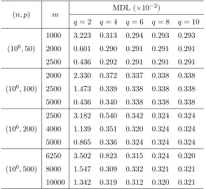
In this section, we investigate the performance of the MDL estimator for varying dimension

p. In Table 3, we choose a large sample sizen= 106, and vary the dimensionpand the batch sizem. We report the L2 error of the MDL estimator with different number of iterations.

From the result we can see that our proposed estimator maintains good performance under large scale settings. TheL2 error of the MDL estimator becomes small in all settings and

(m, p) n (×103)

MDL Na¨ıve-DC Oracle

bias2 (×10−4)

var

(×10−4)

bias2 (×10−4)

var

(×10−4)

bias2 (×10−4)

var

(×10−4)

(100,4)

2 1.782 55.412 58.377 24.912 0.017 13.382

3 0.221 28.275 60.877 17.707 0.046 8.557

5 0.120 12.694 60.696 10.267 0.020 5.016

8 0.005 4.056 58.806 6.213 0.028 3.244

10 0.008 3.054 62.461 4.919 0.025 2.568

20 0.006 1.400 61.609 2.589 0.005 1.325

30 0.000 1.611 60.540 1.754 0.002 0.773

(1000,20)

20 0.002 0.355 1.075 0.334 0.001 0.294

30 0.001 0.207 1.148 0.236 0.001 0.194

50 0.001 0.122 1.147 0.144 0.001 0.121

80 0.000 0.072 1.118 0.082 0.000 0.072

100 0.000 0.054 1.090 0.060 0.000 0.053

Table 2: Bias and variance analysis of MDL, Na¨ıve-DC and oracle estimator with different sample size nwhen number of aggregationsq = 6.

5.4. Sensitivity Analysis of the Bandwidth Constant C0

Finally, we report the simulation study to show that the algorithm is not sensitive to the choice ofC0in bandwidthhg wherehg =C0max(

p

p/n,(p/m)2g−2). We setn= 104,p= 4 withm∈ {50,100}and n= 105,p= 20 withm∈ {500,1000}. The constantC0 is selected

from{0.5,1,2,5,10}. We plot theL2error of the MDL estimator at each iteration step with

different choices of C0. We also plot the L2 error of the Na¨ıve-DC estimator (the dashed

line) and the oracle estimator (the black line) as horizontal lines for comparison. Figure 5 shows that the proposed estimator exhibits good performance for all choices of C0 after a

few rounds of iterations and finally achieves the L2 errors which are close to the L2 error

of the oracle estimator.

6. Conclusions and Future Works

(n, p) m MDL (×10 −2₎

q= 2 q = 4 q = 6 q= 8 q= 10

(106,50)

1000 3.223 0.313 0.294 0.293 0.293

2000 0.601 0.290 0.291 0.291 0.291

2500 0.436 0.292 0.291 0.291 0.291

(106,100)

2000 2.330 0.372 0.337 0.338 0.338

2500 1.473 0.339 0.338 0.338 0.338

5000 0.436 0.340 0.338 0.338 0.338

(106,200)

2500 3.182 0.540 0.342 0.324 0.324

4000 1.139 0.351 0.320 0.324 0.324

5000 0.865 0.336 0.324 0.324 0.324

(106,500)

6250 3.502 0.823 0.315 0.324 0.320

8000 1.547 0.309 0.332 0.321 0.321

10000 1.342 0.319 0.312 0.320 0.321

Table 3: Comparison of the L2 error under different dimensionality p and batch size m.

The sample size is fixed ton= 106, and the number of iterationsq = 10.

statistical efficiency as the classical linear SVM estimator using all the data. In our theo-retical results in Theorem 1, the term (_mp)2q−1 corresponds to the convergence rate of the bias. An interesting theoretical open problem is that whether the rate of the bias is optimal. Note that according to Lemma 1, the expectation of the bias is bounded by a2_n (with the choice of bandwidthh=an). We conjecture that the rate of the biasa2nis optimal, but we

leave this conjecture for future investigation.

This work only serves as the first step towards distributed inference for SVM, which is an important area that bridges statistics and machine learning. In the future, we would like to further establish unified computational approaches and theoretical tools for statistical inference for other types of SVM problems, such asLq-penalized SVM (see ,e.g., Liu et al.

(2007)), high-dimensional SVM (see, Peng et al. (2016); Zhang et al. (2016b)), and more general kernel-based SVM.

Acknowledgments

(a)p= 4,n= 104_{, m= 50 case (b)p= 4, n= 10}4_{,m= 100 case}

(c)p= 20,n= 105_{,m= 500 case (d)p= 20,n= 10}5_{,m= 1000 case}

Figure 5: L2 error of the MDL estimator with different C0. Dashed lines show the

perfor-mance of the Na¨ıve-DC approach and the black solid line shows the perforperfor-mance of the oracle estimator. Other colored lines show the performance of the MDL estimator with different choices of constants in the bandwidth.

Appendix A. Proofs for Results

In this appendix, we provide the proofs of the results.

A.1. Technical Lemmas

Before proving the theorems and propositions, we first introduce three technical lemmas, which will be used in our proof.

Lemma 1 Suppose that conditions (C0)-(C4) hold. For any v˜ ∈_Rp+1 _{with kv˜k}

2 = 1, we

have

E

(

Yv˜TfX H

1−YfX T

e

α

h

!

+ 1−YfX

T e

β∗

h H

0 1−YfX T

e

α

h

!!)

=O(h2+kα_e−βe ∗

k2₂),

uniformly in kα_e−βe ∗

k2 ≤an with any an→0.

Proof of Lemma 1. Without loss of generality, assume that β₁∗≥c. Thenα1≥c/2. For

any v∈Rp,

E

Y(v0+vTX)H

1−Y(α0+XTα) h

=π+ Z

Rp

(v0+vTx)H

1−α0−xTα h

f(x)dx−π− Z

Rp

(v0+vTx)H

1 +α0+xTα h

g(x)dx.

We have

Z

Rp

(v0+vTx)H

1−α0−xTα h

f(x)dx

=

Z

Rp−1

Z

R

(v0+v1x1+vT−1x−1)H

1−α0−x1α1−xT−1α−1 h

!

f(x1,x−1)dx1dx−1

=− h

α1 Z

Rp−1

f−1(x−1) Z

R

v0+v1

1−α0−xT−1α−1−hy α1

+vT−1x−1 !

×f 1−α0−x T

−1α−1−hy α1

|x−1 !

DefineG(t|x−1) =R_−∞t xf(x|x−1)dx. SinceR

R|x|f(x|x−1)dx <∞, we haveG(−∞|x−1) =

0. Then,

−

Z

R

v1

1−α0−xT−1α−1−hy α1

f 1−α0−x T

−1α−1−hy α1

|x−1 !

H(y)dy

=α1

h v1

Z

R

H(y)dG 1−α0−x T

−1α−1−hy α1

|x−1 !

=−α1 h v1

Z 1 −1

G 1−α0−x T

−1α−1−hy α1

|x−1 !

H0(y)dy

=−α1 h v1G

1−β∗₀−xT₋₁β∗−1 β₁∗ |x−1

!

−α1 h v1

Z 1 −1

1−β₀∗−xT₋₁β∗−1

β₁∗ f

1−β₀∗−xT₋₁β∗−1 β₁∗ |x−1

!

∆(α,β∗,x−1, y)H0(y)dy

+O(1)α1

h v1

Z 1 −1

∆2(α,β∗,x−1, y)|H0(y)|dy,

where

∆(α,β∗,x−1, y) =

1−α0−xT−1α−1−hy α1

−1−β

∗

0 −xT−1β∗−1 β₁∗ ,

and the inequality|xf(x|x−1)−yf(y|x−1)| ≤C|x−y|followed from Condition (C2). Also,

−

Z

R

(v0+vT−1x−1)f

1−α0−xT−1α−1−hy α1

|x−1 !

H(y)dy

=− α1 h

Z 1 −1

(v0+vT−1x−1)F

1−α0−xT−1α−1−hy α1

|x−1 !

H0(y)dy

=− α1

h (v0+v T

−1x−1)F

1−β₀∗−xT₋₁β∗₋₁

β₁∗ |x−1

!

− α1 h

Z 1 −1

(v0+vT−1x−1)f

1−β₀∗−xT₋₁β∗₋₁

β₁∗ |x−1

!

∆(α,β∗,x−1, y)H0(y)dy

+O(1)α1

h

Z 1 −1

|v0+vT−1x−1|∆2(α,β∗,x−1, y)|H0(y)|dy.

Next we consider

E

Y(v0+vTX)

1−Y(β₀∗+XTβ∗)

h H

0

1−Y(α0+XTα) h

=π+ Z

Rp

(v0+vTx)

1−β₀∗−xTβ∗

h H

0

1−α0−xTα h

f(x)dx

−π− Z

Rp

(v0+vTx)

1 +β₀∗+xTβ∗

h H

0

1 +α0+xTα h

We have

Z

Rp

(v0+vTx)

1−β₀∗−xTβ∗

h H

0

1−α0−xTα h

f(x)dx

=− 1

α1 Z

Rp−1

f−1(x−1) Z

R

v0+v1

1−α0−xT−1α−1−hy α1

+vT₋₁x−1 !

× 1−β₀∗−β₁∗1−α0−x T

−1α−1−hy α1

−xT₋₁β∗₋₁

!

×f 1−α0−x T

−1α−1−hy α1

|x−1 !

H0(y)dydx−1.

Note that − 1 α1 Z R

v0+v1

1−α0−xT−1α−1−hy

α1

+vT₋1x−1

×

1−β₀∗−β₁∗1−α0−x

T

−1α−1−hy

α1

−xT₋₁β∗₋₁

×f

_1−α

0−xT−1α−1−hy

α1

|x−1

H0(y)dy

=β ∗ 1 α1 Z R

v0+v1

1−α0−xT−1α−1−hy

α1

+vT₋₁x−1

∆(α,β∗,x−1, y)

×f

_1−α

0−xT−1α−1−hy

α1

|x−1

H0(y)dy

=

Z

R

v0+v1

1−α0−xT−1α−1−hy

α1

+vT₋₁x−1

∆(α,β∗,x−1, y)

×f

_1−β∗

0−xT−1β ∗ −1

β∗₁ |x−1

H0(y)dy

+O(1)

Z R

v0+v1

1−α0−xT−1α−1−hy

α1

+vT₋₁x−1

∆2(α,β∗,x−1, y)|H0(y)|dy

+O(1)|β

∗ 1−α1|

α1 Z R

v0+v1

1−α0−xT−1α−1−hy

α1

+vT₋₁x−1

∆(α,β∗,x−1, y)|H0(y)|dy

=

Z

R

v0+v1

1−β0∗−xT−1β ∗ −1

β1

+vT₋₁x−1

∆(α,β∗,x−1, y)f

_1−β∗

0−xT−1β ∗ −1

β₁∗ |x−1

H0(y)dy

+O(1)

Z R

v0+v1

1−α0−xT−1α−1−hy

α1

+vT₋₁x−1

∆2(α,β∗,x−1, y)|H0(y)|dy

+O(1)|β

∗ 1−α1|

α1 Z R

v0+v1

1−α0−xT−1α−1−hy

α1

+vT₋₁x−1

∆(α,β∗,x−1, y)|H0(y)|dy

+O(1)

Z

R

∆2(α,β∗,x−1, y)|H0(y)|dy.

Note that

|∆(α,β∗,x−1, y)| ≤C h+|xT−1(α−1−β∗−1)|+|1−β∗0−xT−1β∗−1||α1−β∗1|+|α0−β0∗|