Article
Detecting the Spatially Non-Stationary Relationships
between Housing Price and Its Determinants in
China: Guide for Housing Market Sustainability
Yanchuan Mou1,3, Qingsong He2,3,* ID and Bo Zhou1,*
1 College of Architecture and Environment, Sichuan University, No. 29 Jiuyanqiao Wangjiang Road,
Chengdu 610064, China; [email protected]
2 School of Resource and Environmental Science, Wuhan University, 129 Luoyu Road, Wuhan 430079, China 3 Department of City and Regional Planning, University of North Carolina at Chapel Hill,
Chapel Hill, NC 27599, USA
* Correspondence: [email protected] (Q.H.); [email protected] (B.Z.)
Received: 18 August 2017; Accepted: 7 October 2017; Published: 11 October 2017
Abstract:Given the rapidly developing processes in the housing market of China, the significant regional difference in housing prices has become a serious issue that requires a further understanding of the underlying mechanisms. Most of the extant regression models are standard global modeling techniques that do not take spatial non-stationarity into consideration, thereby making them unable to reflect the spatial nature of the data and introducing significant bias into the prediction results. In this study, the geographically weighted regression model (GWR) was applied to examine the local association between housing price and its potential determinants, which were selected in view of the housing supply and demand in 338 cities across mainland China. Non-stationary relationships were obtained, and such observation could be summarized as follows: (1) the associations between land price and housing price are all significant and positive yet having different magnitudes; (2) the relationship between supplied amount of residential land and housing price is not statistically significant for 272 of the 338 cities, thereby indicating that the adjustment of supplied land has a slight effect on housing price for most cities; and (3) the significance, direction, and magnitude of the relationships between the other three factors (i.e., urbanization rate, average wage of urban employees, proportion of renters) and housing price vary across the 338 cities. Based on these findings, this paper discusses some key issues relating to the spatial variations, combined with local economic conditions and suggests housing regulation policies that could facilitate the sustainable development of the Chinese housing market.
Keywords: housing price; spatial non-stationarity; geographically weighted regression; Chinese cities; sustainability
1. Introduction
Housing is one of the most basic needs for human settlement and development. The housing market is an important indicator of the degree of economic development and quality of life in a particular area. The Chinese government advanced a “housing system reform” policy in 1998, thereby ending the welfare housing distribution system [1–3]. Prior to this reform, the state or state-owned enterprises (danwei) provided housing for their workers for free or at an extremely low price. From then on, most Chinese families needed to turn to the commercial housing market for their housing needs, hence greatly stimulating and promoting the Chinese housing market. According to National Bureau of Statistic, the trading volume and average price of Chinese commodity housing were 1.22×10⁸ m2and 1854 yuan/ m2in 1998, respectively [4], and they soared to 1.57×10⁹ m2and
7476 yuan/m2in 2016. These changes indicate a respective increase of 1187% and 262% and highlights the rapid growth of the Chinese housing market.
As the housing market continued to develop, the spatial difference in housing prices across cities became increasingly apparent [2,5–7]. From 2006 to 2015, the housing prices in first-tier cities experienced an annual growth rate of 15% to 20% (e.g., an average annual increase of 20% in Shenzhen and 17% in Shanghai and Beijing). In contrast, the housing prices in inland cities, such as Guiyang, Xining, and Kunming, experienced an average annual growth rate of 2% to 5% [8]. Wang et al. [9] observed a significant difference between inland cities and southwest coastal urban areas in terms of their housing price and price-to-income ratio by using data from 286 prefecture-level cities across China in 2009. Further research revealed a similar phenomenon, that is, that those counties with high housing prices were mainly concentrated in the southeast coast and the Beijing–Tianjin metropolitan area. The average housing price in the eastern region was also much higher than that in the western and central regions [10]. These spatial differences in housing prices reflect the spatial heterogeneity in socio-economic development, leading to inflation and imposing pressure on housing and land costs. Such pressure may compromise national economic policies when spreading across the entire country [11]. Therefore, reducing the spatial inequality in housing price and promoting the sustainable development of Chinese housing market are crucial.
Two important research topics—the driving mechanism of housing price change and the formulation of regulation policies for the sustainable development—have been emphasized in recent years. Numerous scholars have conducted broad and in-depth research on the determinants of housing price and their effects. Referring to panel data from 29 provinces in China from 1995 to 2005, Chen et al. [4] found that rural–urban migration significantly affected housing price. Wang and Zhang [8] developed equilibrium models to explain the role of fundamental factors in the Chinese housing market at the prefectural level. Wang et al. [10] analyzed the direction and strength of the relationship between housing price and its determinants at the county-level in China by using a spatial regression technique. The results identified the positive effect from six determinants (i.e., land price, renter proportion, floating population, wage level, housing market, and city service level) and negative influence from living space. These studies examined the relationship between housing price and its determinants in China at the provincial, prefectural, and county levels and were all based on ordinary least squares (OLS) regression or spatial error models (SEM) and spatial lag models (SLM). All of these models are global models. OLS linear regression posits that the cause–effect relationship will be the same across the entire study area. Although SEM and SLM consider proximity effects, they continue to assume spatial stationarity as a prerequisite. Stationary coefficient models have parameters that are essentially computed as “average” values over all locations. However, housing is typically a spatially heterogeneous commodity because of its immovability [12]. Therefore, the varying economic conditions, natural resource endowments, and traffic conditions across cities can lead to a situation in which the relationships between dependent and independent variables are not constant over space and conversely vary with the spatial context in reality [13–15]. This type of spatial variability is known as spatial non-stationarity [16]. Global models that ignore spatial non-stationarity cannot reflect local associations and may obscure regional variations in the relationship between housing price and its determinants, resulting in reducing their real application value [17]. To enhance the understanding of the sophisticated associations between housing price and its determinants, specific local techniques are assumed to be used to capture spatial variability and non-stationarity.
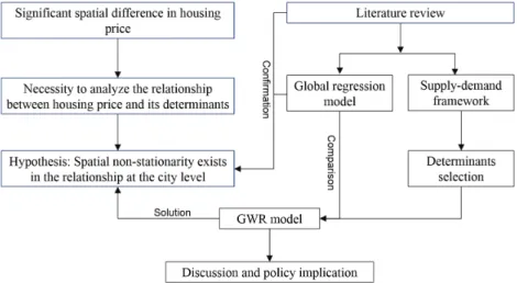
transportation [21], modeling daily fire danger in northeast China [22], and quantifying spatial non-stationarity between the distribution of alcohol and violence [23]. These studies have justified GWR as an excellent descriptor of spatial variability. China is facing serious imbalances in its regional development and considerable disparities in its housing prices, demographic structure, economic development, and level of city services. In this context, GWR is applied to quantify the spatial non-stationary relationships between housing price and its determinants at the city level, and relative housing market control policy discussions are made accordingly. The conceptual framework is shown in Figure1.
The remainder of the article is organized as follows. Section2reviews the related literature and presents an overview of the determinants of housing price based on a supply-demand framework. Section3selects the applied variables to construct the underlying model and introduces the data sources. Section4discusses the research methodology in detail. Section5provides the regression results, compares the performance of various models, and discusses the spatial patterns in the context of local economic conditions. Section6draws conclusions from the findings and proposes policies for ensuring the sustainability of the Chinese housing market.
Sustainability 2017, 9, 1826 3 of 17
GWR as an excellent descriptor of spatial variability. China is facing serious imbalances in its regional development and considerable disparities in its housing prices, demographic structure, economic development, and level of city services. In this context, GWR is applied to quantify the spatial non-stationary relationships between housing price and its determinants at the city level, and relative housing market control policy discussions are made accordingly. The conceptual framework is shown in Figure 1.
The remainder of the article is organized as follows. Section 2 reviews the related literature and presents an overview of the determinants of housing price based on a supply-demand framework. Section 3 selects the applied variables to construct the underlying model and introduces the data sources. Section 4 discusses the research methodology in detail. Section 5 provides the regression results, compares the performance of various models, and discusses the spatial patterns in the context of local economic conditions. Section 6 draws conclusions from the findings and proposes policies for ensuring the sustainability of the Chinese housing market.
Figure 1. Conceptual framework.
2. Literature Review
Housing is not only regulated by the market mechanism, but also to some extent, by the government. Therefore, different economic systems and levels have led to variations in the existing housing market. In this context, the comparison of the housing market with the same or similar political/institutional framework is more appropriate. This section provides a brief review of determinants of housing price adopted in relevant studies focusing on Chinese housing market. An increasing number of studies have been conducted based on a supply-demand framework. Chow and Niu [24] applied a standard housing demand-supply framework to explain the rapid growth in the urban housing price in China based on annual data from 1987 to 2006, and concluded that the housing price change could be well explained by a demand and supply framework using national aggregate data. l. Similarly, Wang and Zhang [8] proposed an empirical approach that considers the four fundamental factors (i.e., urban hukou population, wage income, urban land supply, and construction costs) of demand-supply at both the city- and project-level. They found that the selected factors could account for a large proportion of the actual housing price appreciation in most cities.. The most widely used socioeconomic and demographic factors are summarized in Table 1 based on a demand-supply framework.
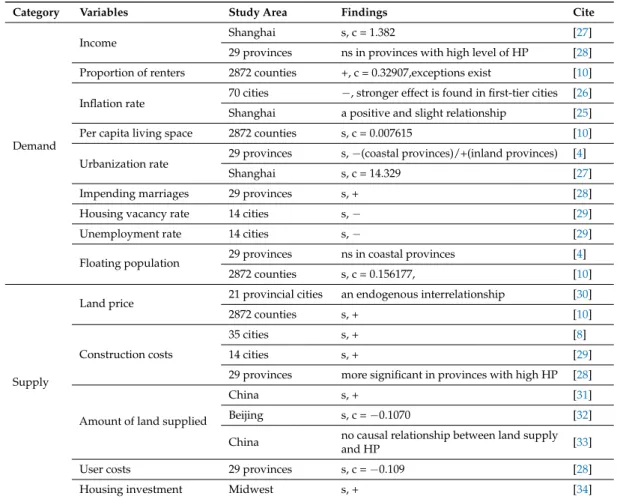
Table 1 shows considerable variations for the same variable across different studies. Zou and Chau [25] investigated the impacts of inflation rate on housing price in Shanghai based on the monthly data for the period of 2005–2010 and found a positive and slight relationship. Zhang et al. [26] divided the 70 large and medium-sized cities in China into three tiers based on key factors (i.e., transportation system, infrastructure construction, economic environment, and cultural
Figure 1.Conceptual framework.
2. Literature Review
Housing is not only regulated by the market mechanism, but also to some extent, by the government. Therefore, different economic systems and levels have led to variations in the existing housing market. In this context, the comparison of the housing market with the same or similar political/institutional framework is more appropriate. This section provides a brief review of determinants of housing price adopted in relevant studies focusing on Chinese housing market. An increasing number of studies have been conducted based on a supply-demand framework. Chow and Niu [24] applied a standard housing demand-supply framework to explain the rapid growth in the urban housing price in China based on annual data from 1987 to 2006, and concluded that the housing price change could be well explained by a demand and supply framework using national aggregate data. l. Similarly, Wang and Zhang [8] proposed an empirical approach that considers the four fundamental factors (i.e., urbanhukoupopulation, wage income, urban land supply, and construction costs) of demand-supply at both the city- and project-level. They found that the selected factors could account for a large proportion of the actual housing price appreciation in most cities.. The most widely used socioeconomic and demographic factors are summarized in Table1 based on a demand-supply framework.
the 70 large and medium-sized cities in China into three tiers based on key factors (i.e., transportation system, infrastructure construction, economic environment, and cultural significance), and then empirically studied the relationship between housing price and macroeconomy. They found that the effect of inflation rate on the housing prices was positive initially and then became negative, and the more significant negative effect was found in first-tier cities. In terms of the floating population, Wang et al. [10] identified it as a significant positive factor for housing price. Chen et al. [4] divided the selected cities into coastal and inland ones, and found that there is significant negative correlation for inland cities while insignificant for coastal cities. The results provide strong evidence to confirm the hypothesis mentioned in first section that there are spatial variations in the relationship between housing price and its determinants. Global statistics do not give useful insights into the issue and may produce misleading results when examining the relationship. Previous studies that reveal such non-stationary relationships have dealt with spatial heterogeneity by delineating the cities into distinct geographic areas or different city tiers and estimating the global regression separately. However, city classification is often problematic in practice and hinders researchers from making generalizations about the uncertainty of a broader and dynamic housing market [17]. In this context, we use a better regression model, GWR, which enables us to estimate local coefficients to deal effectively with spatial non-stationarity.
Table 1.Main variables identified in the literature review.
Category Variables Study Area Findings Cite
Demand
Income Shanghai s, c = 1.382 [27]
29 provinces ns in provinces with high level of HP [28]
Proportion of renters 2872 counties +, c = 0.32907,exceptions exist [10]
Inflation rate 70 cities −, stronger effect is found in first-tier cities [26]
Shanghai a positive and slight relationship [25]
Per capita living space 2872 counties s, c = 0.007615 [10]
Urbanization rate 29 provinces s,
−(coastal provinces)/+(inland provinces) [4]
Shanghai s, c = 14.329 [27]
Impending marriages 29 provinces s, + [28]
Housing vacancy rate 14 cities s,− [29]
Unemployment rate 14 cities s,− [29]
Floating population 29 provinces ns in coastal provinces [4]
2872 counties s, c = 0.156177, [10]
Supply
Land price 21 provincial cities an endogenous interrelationship [30]
2872 counties s, + [10]
Construction costs
35 cities s, + [8]
14 cities s, + [29]
29 provinces more significant in provinces with high HP [28]
Amount of land supplied
China s, + [31]
Beijing s, c =−0.1070 [32]
China no causal relationship between land supply
and HP [33]
User costs 29 provinces s, c =−0.109 [28]
Housing investment Midwest s, + [34]
3. Variables and Data Processing
3.1. Variables
Based on the findings from the literature review, we use a standard supply-demand framework to understand how different variables affect the housing price in different cities. In modeling the demand side, purchasing power and impending housing buyers are two vital factors. Therefore, we select urbanization rate, the average wage of urban employees and the proportion of renters as demand variables. With respect to the housing supply, land is an essential factor for house construction. Urban residential land and housing markets are two relevant markets [30]. Thus, land price and the supplied amount of residential land are selected as variables. The modifications and uses of the selected factors are discussed as follows:
Urbanization Rate(UR):Urbanization generally refers to the process of migration flows into cities and the transformation process of rural areas into urban areas. The urbanization rate basically reflects the level of economic development and social progress of a city, to a certain extent. One of the most obvious features of urbanization in China is the large flow of rural-city migrants, providing labor for economic growth while also expanding the demand for housing. The significant regional difference in urbanization rate (e.g., the UR of Shenzhen is 100%, while Baoshan is only 28.15%) might lead to variations of the results.
Average Wage of Urban Employees(AWUE):Wage level is an important indicator of the income level that comprehensively reflects the purchasing power of urban residents. Wage level has been widely used as an explanatory factor for changes in housing price [35,36]. In general, high income provides people with financial support when purchasing a house, thereby subsequently increasing both the housing demand and housing price.
Proportion of Renters(PR):Given their traditional deep-rooted concept of home ownership, the Chinese people not only view housing as a place of residence but also attach social meaning to it, such as happiness and safety [37]. Therefore, most urban residents purchase a house in the city where they work if their financial condition permits. Rental housing is widely recognized as a “stepping stone” to social housing and eventual owner occupancy [38]. More than 100 million renters have been recorded in China by the end of 2016 (MOHURD), and these renters represent a large proportion of the housing demand according to Goodman [39]. The change in housing demand will cause housing price fluctuation.
Land Price(LP):Three different influence mechanisms between housing price and land price are described. From a cost-driven perspective, housing price consists of land cost, construction cost, related taxes, and developer profits. The ratio of land cost to housing price increased from 9% in 1998 to 24.3% in 2011 [10]. As a major component, land price is supposed to affect housing price. From a supply-demand perspective, when the housing market demand exceeds supply, both the housing and land prices will increase. The third mechanism is based on the perspective that land and house prices have a mutually causal relationship [30]. Therefore, land price is assumed to have a positive correlation with housing price.
3.2. Study Area
This research uses 334 prefectural level cities(di ji shi)and 4 municipalities(zhi xia shi), and the total is 338 cities as our study area. A general definition about Chinese city system, which has been long defined administratively, is introduced: Municipalities directly under the central government have the same political, economic and jurisdictional rights as provinces , and prefectural-level cities rank below provinces but above counties (A comprehensive review of Chinese city systems is presented in Li’s research [41]). In general, a prefectural level city includes city-governed districts and its surrounding regions such as the seats of counties, and there is a significant differences in their housing price. For example, Chengdu City consists of city-governed districts, 5 county-level cities, and 4 counties, and the housing prices range from 3791 yuan/m2to 10,780 yuan/m2, as shown in Figure2. The housing price of counties and county-level cities is obviously much lower than that in city-governed districts. Studies that focus on the entire city will produce misleading results. Therefore, we only take the city-governed districts of the selected cities into account to make the results more reliable. The administrative boundaries are derived from the Second Land Use Survey of China.
Sustainability 2017, 9, 1826 6 of 17
Figure 2. Housing prices in Chengdu City.
3.3. Data Sources and Processing
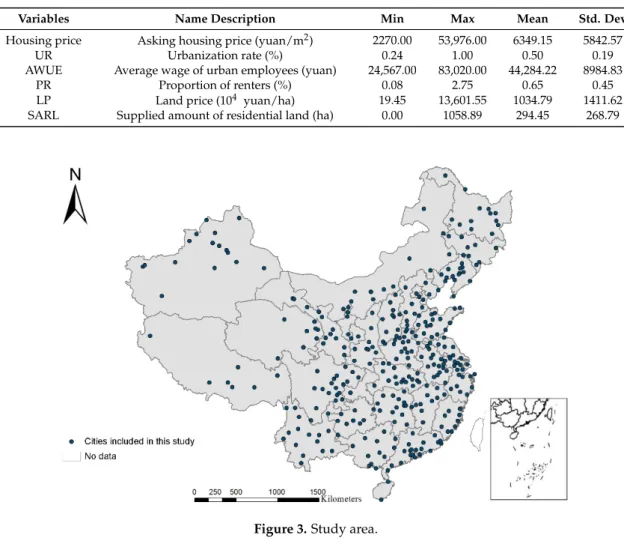
Because transaction price for most cities in China is inaccessible, we used asking price, which is widely used in hedonic price modeling to estimate housing price and has been proven to generate robust results [21,42]. Taking Shanghai as an example, asking and transaction price are highly correlated with a possible swing of ±10% [43]. Therefore, the effect of the determinants on housing price can be examined without any significant errors by looking at asking price. Data on housing prices were obtained from the website http://sjz.anjuke.com/, which is the most important housing transaction website in China with more than three million online housing records. A total of 121,512 commercial housing records, including the location (in latitude and longitude format) and asking price information for November 2016, were collected using crawling techniques. Given the large number of housing price records collected for each city, mean and median value were calculated respectively. Compared with the transactional price of 30 major cities for November 2016, which was obtained at http://fdc.fang.com/, the world’s largest housing network platform, the mean value is closer to transaction price with a comparative gentle fluctuation. The site of municipal governments are used to represent the spatial location of mean housing price of 338 cities because it is impossible to precisely define the points on the map (Figure 3).
The data for the independent variables were obtained from statistical yearbooks. Specifically, AWUE data were collected from the 2016 China Statistical Yearbook for the Regional Economy, while UR and PR data were collected from the 2016 Statistical Yearbook for each city. After the acquisition of land use rights, developers usually need three years to transform the site into housing units, and land-related indicators are known to have a three-year lag effect on housing price [44]. LP and SARL data were collected from the 2013 Land and Resources China Statistical Yearbook. The descriptive statistics for all variables are shown in Table 2.
Table 2. Descriptive statistics for the variables.
Variables Name Description Min Max Mean Std. Dev
Housing price Asking housing price (yuan/m2) 2270.00 53,976.00 6349.15 5842.57
UR Urbanization rate (%) 0.24 1.00 0.50 0.19
AWUE Average wage of urban employees (yuan) 24,567.00 83,020.00 44,284.22 8984.83
PR Proportion of renters (%) 0.08 2.75 0.65 0.45
LP Land price (10 yuan/ha) 19.45 13,601.55 1034.79 1411.62 SARL Supplied amount of residential land (ha) 0.00 1058.89 294.45 268.79
0 2000 4000 6000 8000 10000 12000
City-governed districts Dujiangyan city Jianyang city Pujiang city Chongzhou city Pengzhou city Xinjin county Qionglai county Jintang county Dayi county
Housing price (yuan/㎡)
Figure 2.Housing prices in Chengdu City.
3.3. Data Sources and Processing
The data for the independent variables were obtained from statistical yearbooks. Specifically, AWUE data were collected from the 2016 China Statistical Yearbook for the Regional Economy, while UR and PR data were collected from the 2016 Statistical Yearbook for each city. After the acquisition of land use rights, developers usually need three years to transform the site into housing units, and land-related indicators are known to have a three-year lag effect on housing price [44]. LP and SARL data were collected from the 2013 Land and Resources China Statistical Yearbook. The descriptive statistics for all variables are shown in Table2.
Table 2.Descriptive statistics for the variables.
Variables Name Description Min Max Mean Std. Dev
Housing price Asking housing price (yuan/m2) 2270.00 53,976.00 6349.15 5842.57 UR Urbanization rate (%) 0.24 1.00 0.50 0.19 AWUE Average wage of urban employees (yuan) 24,567.00 83,020.00 44,284.22 8984.83
PR Proportion of renters (%) 0.08 2.75 0.65 0.45 LP Land price (104 yuan/ha) 19.45 13,601.55 1034.79 1411.62 SARL Supplied amount of residential land (ha) 0.00 1058.89 294.45 268.79
Sustainability 2017, 9, 1826 7 of 17
Figure 3. Study area.
4. Methods
4.1. Model Fitting
The min–max normalization method is applied to normalize all variables. Then a Pearson’s correlation and variance inflation factor (VIF) are applied to diagnose and avoid potential multi-collinearity problems among the independent variables. The results indicate that all pairs of variables has a significant and relatively weak correlation (<0.5), and the VIF values for UR, AWUE, PR, LP, and SARL are 1.1075, 1.5682, 1.4444, 1.2846, and 1.1124 (all of them are much less than 10) respectively. In this case, all these variables are kept in the further regression analysis. Next, we use the Add Join feature in ArcGIS to link the data associated with each variable to the city spatial data for subsequent modeling and analysis. We also perform OLS for comparison and analyze the necessity of GWR based on OLS diagnostics. The Koenker (BP) statistic and Jarque–Bera are applied to assess the model stationarity and bias, respectively. Both OLS and GWR are estimated in ArcGIS 10.2. The GWR 4.0 software is used to derive local t-values that indicate the significance of local parameters in order to yield a meaning explanation of the results.
4.2. Model Evaluation
The measures of , adjusted , and residual squares are used to evaluate the performance of OLS and GWR. According to the evaluation criteria proposed by Fotheringham [18], for the same sample data, if the difference in the value between two models is greater than 3, then the model with a lower value has a better fit for the observed data. A higher adjusted and lower residual squares also indicate a better model. The spatial autocorrelation (Moran’s I) tool is also used to examine the patterns in the OLS and GWR model residuals. We calculate the Moran’s index at the significance level of 0.05. A larger Moran’s index indicates a greater dependency on the residuals, thereby indicating that the model cannot adequately explain the change in the dependent variable [45]. On the contrary, a smaller Moran’s index indicates a better model.
Figure 3.Study area.
4. Methods
4.1. Model Fitting
4.0 software is used to derive localt-values that indicate the significance of local parameters in order to yield a meaning explanation of the results.
4.2. Model Evaluation
The measures ofAICC, adjustedR2, and residual squares are used to evaluate the performance of OLS and GWR. According to the evaluation criteria proposed by Fotheringham [18], for the same sample data, if the difference in theAICCvalue between two models is greater than 3, then the model with a lower value has a better fit for the observed data. A higher adjustedR2and lower residual squares also indicate a better model. The spatial autocorrelation (Moran’s I) tool is also used to examine the patterns in the OLS and GWR model residuals. We calculate the Moran’s index at the significance level of 0.05. A larger Moran’s index indicates a greater dependency on the residuals, thereby indicating that the model cannot adequately explain the change in the dependent variable [45]. On the contrary, a smaller Moran’s index indicates a better model.
4.3. Geographically Weighted Regression
GWR (Equation (1)) extends the OLS approach by embedding the geographic location of the observation into the model. Each parameter is estimated in space to improve the goodness of fit of the model greatly.
yi=β0(ui,vi) +
∑
kβk(ui,vi)xik+εi, (1)
where(ui,vi)represents the spatial coordinates,β0(ui,vi)is the intercept, andβk(ui,vi)is the local coefficient ofkvariable at theipoint. The coefficients are estimated using weighted least squares (WLS) (Equation (2)) at each location(ui,vi), where εirepresents the error term,εi∼N 0,σ2;
βj(ui,vi) =XtW(ui,vi)X −1
XtW(ui,vi)y, (2)
whereW(ui,vi)is the spatial weighting matrix. According to the first law of geography, the points that are located closer to the regression coordinates(ui,vi)contribute more in the estimation of the parameter. In this study, we use the Gauss function to determine the weighting matrix as follows (Equation (3)):
wij=exp h
− dij/b2 i
, (3)
wheredijis the Euclidean distance between the location of observationiand location j,brepresents the bandwidth of sampled observations, andwijis a continuous monotone decreasing function ofdij. Ifdij =0, thenwij =1.
GWR is sensitive to the choice of bandwidth. A wide bandwidth will generate results that are similar to a global regression model. Conversely, a small bandwidth will lead to large variances in the estimators. The distribution of observed cities is inhomogeneous, and the density of cities in the eastern region is much higher than that in the western region. We choose an adaptive spatial kernel, that is, the bandwidth becomes a function of the number of nearest neighbors so that each local observation is based on the same number of cities. Thus, the bandwidth distance will become larger where the cities are sparsely distributed and smaller where the cities are densely distributed. To obtain the optimal bandwidth, the adjusted value of the Akaike Information Criterion (AICc) is used. The resulting bandwidth is 87 observations. AICc is expressed as follows:
AICC=2nln(σˆ) +nln(2π) +n n+tr(S)
n−2−tr(S), (4)
whereσis the maximum likelihood estimator of the variance of random error, andtr(S)is the trace of
5. Results and Discussion
5.1. Model Performance and Estimates
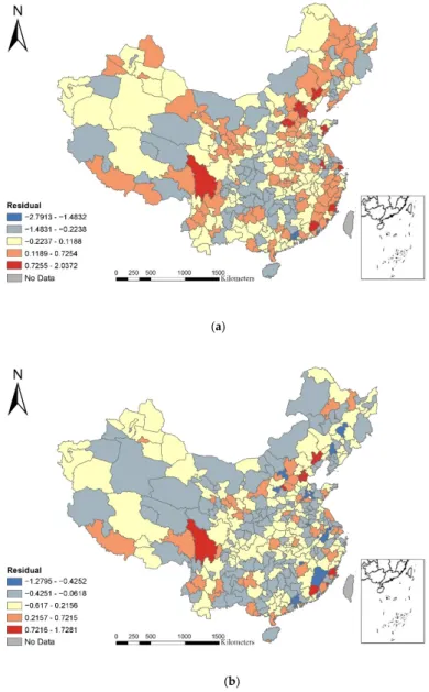
Based on the OLS diagnosis, the BP statistic is statistically significant (p= 0.000), indicating that the association between determinants and the predicted housing price varies along with changes in magnitude and that the model is inconsistent spatially in the data space. Thep-value of the Jarque–Bera statistic is smaller than 0.01, showing that the residuals are randomly distributed and that a biased model is obtained. Table3summarizes the performance of the OLS and GWR models. The GWR model accounts for 87.1% of the change in housing price, which is 7.5% higher than OLS. The residual square values for GWR are lower than those for OLS, indicating that the GWR model has a closer fit to the observed data. The AICc value for GWR is 322.042, which is much lower than the comparative value for OLS. Figure4a,b show the patterns in the OLS and GWR model residuals, and their Moran’s I equal to 0.099 (Zscore = 7.237) and 0.017 (Zscore = 1.391), respectively. A strong tendency of OLS model residuals toward clustering becomes noticeable. These results show that GWR is more suitable and powerful than OLS in explaining the relationship between housing price and its determinants.
Sustainability 2017, 9, 1826 9 of 17
GWR is more suitable and powerful than OLS in explaining the relationship between housing price and its determinants.
Table 3. Model performance comparison.
Models Adjusted Residual Squares
OLS 432.410 0.796 68.08
GWR 322.042 0.871 34.94
(a)
(b)
Figure 4. (a) Plot of ordinary least squares (OLS) residuals; (b) Plot of geographically weighted regression model (GWR) residuals.
5.2. Discussion of Estimated Coefficients
Table 3.Model performance comparison.
Models AICc AdjustedR2 Residual Squares
OLS 432.410 0.796 68.08
GWR 322.042 0.871 34.94
5.2. Discussion of Estimated Coefficients
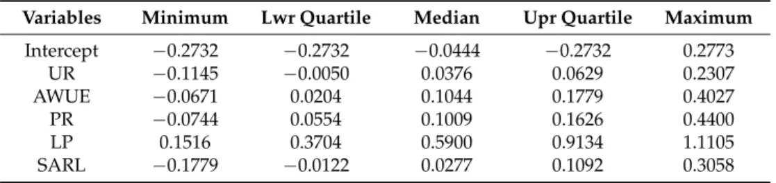
The same data are used in the OLS and GWR models. The OLS model treats the 338 cities as a whole, and the results are assumed to be universal over space. The obtained coefficients are shown in Table4. All variables are significant at the 0.01 level except for SARL. The interpretation here, for the example of AWUE, is that an increase in one point will lead to a 12.27% increase in housing price when other variables are kept constant. By contrast, GWR allows for the estimation of local coefficients and generates a set of coefficients at each of the 338 observations in this study. The coefficients are described by a five-number summary that is based on minimum, lower quartile, median, upper quartile, and maximum values. Table5shows that the parameter estimates for the five variables vary greatly, indicating a significant spatial difference in the relationship between housing price and its determinants.
Table 4.OLS model results.
Variables Coefficient StdError t-Statistic Probability VIF
Intercept 0.0000 0.0244 1.0000 0.0000 –
UR 0.0373 0.0258 5.1345 0.0000 * 1.1075
AWUE 0.1227 0.0307 3.9969 0.0001 * 1.5682
PR 0.1221 0.0295 4.1439 0.0000 * 1.4444
LP 0.7566 0.0278 27.2233 0.0000 * 1.2846
SARL 0.0639 0.0258 2.4720 0.1392 1.1124
* Indicates significance at 0.01 level.
Table 5.GWR model results.
Variables Minimum Lwr Quartile Median Upr Quartile Maximum
Intercept −0.2732 −0.2732 −0.0444 −0.2732 0.2773
UR −0.1145 −0.0050 0.0376 0.0629 0.2307
AWUE −0.0671 0.0204 0.1044 0.1779 0.4027
PR −0.0744 0.0554 0.1009 0.1626 0.4400
LP 0.1516 0.3704 0.5900 0.9134 1.1105
SARL −0.1779 −0.0122 0.0277 0.1092 0.3058
5.3. Spatial Pattern
GWR model results show that the coefficients of UR are statistically significant for 204 of the 338 cities in explaining the changes in housing price and range from−0.1145 to 0.2307 (Figure5a). The results justify the hypothesis mentioned in Section3.1that regional variations in the urbanization rate have certain effects on housing price. Positive effects are obtained except for northern part of China. The strongest effect is found in coastal China and it may be attributed to the fact that given the population concentration and the shortage of land resources, the housing market in coastal cities has become highly competitive. Thus, an increase in urbanization rate will also increase the impending housing buyers and generate increased pressure on the market.
According to the OLS model results, AWUE exerts a small positive effect on housing price with a coefficient value of 0.1227. However, the GWR coefficients range from−0.0671 to 0.4027 (Figure5b), indicating that the direction and magnitude of such association vary across cities. Those cities with the highest coefficients are located in coastal China. These results conform to the previous findings that an increase in disposable income has a greater effect on housing prices in eastern China than on those in western and central China [49]. The wage level in coastal cities is much higher than that in inland cities, thereby providing the necessary financial support to improve owner-occupied housing and stimulate the investment in the housing market. Then, housing demand will increase and drive up housing prices.
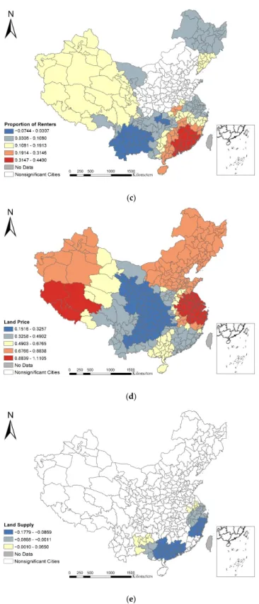
The proportion of renters is widely recognized for its significant positive effect on housing price [10]. In this study, PR has a positive effect on housing price for almost all significant cities (Figure5c). This result can be attributed to three reasons. First, given a rapid increase in housing price, housing not only offers residences for inhabitants but also becomes an asset that provides considerable returns to investors in China [50]. Second, the housing rental market is confusing because of its lack of unified management. Renters, as vulnerable groups in the lease relationship, often encounter obstacles. For example, landlords consistently raise rent against the contract when housing price continues to increase. In addition, purchasing a house offers a means to solve the registered residence(hukou)problem in most cities, with which people are eligible to receive more benefits from the local government. As a result, most renters choose to purchase a house if their financial situation permits, thereby increasing the demand in housing market. Those cities with lower coefficients are divided into two types. The first type of cities with a lower regression coefficient and higher proportion of renters (e.g., Yulin City, Shanxi Province, coefficient =−0.033 and PR = 0.015) are mainly concentrated in Shanxi Province, where the natural resources is abundant, especially in coal and natural gas. According to Wang et al. [10], although a large proportion of short-term migrant workers is present in resource-based cities, they do not exert pressure on the local housing market because they have houses in their rural hometowns and do not intend to settle in the cities. Cities of the second type, which have a lower regression coefficient and proportion of renters (e.g., Baoshan City, Yunnan Province, coefficient = 0.011 and PR = 0.003) are concentrated in the northern and southeastern part of China. This region is relatively less developed, and job opportunities are limited. Those cities with a higher coefficient are concentrated in south coastal China, indicating they are greatly influenced by PR.
and other disadvantages [51]. In addition, the average population growth rate of Tibet from 2000 to 2010 is 1.39%, which is much higher than the national level of 0.57% (NBSC, 2011). The rapid growth rate has caused shortage in land supply, resulting in a rise in land price and comparatively higher ratio of land cost to housing price. Therefore, an increase in land prices will significantly increase the housing prices in Tibet.
The global regression results show that SARL does not significantly affect housing price. However, based on GWR model results, the association between SARL and housing price is statistically significant for 66 of the 338 cities, which are mostly concentrated in coastal provinces (Shanghai, Jiangsu, Zhejiang, Fujian, Guangdong, and Guangxi). Thus, compared with OLS, the GWR technique, which allows data to be analyzed at the local level, is capable of generating more accurate results in this study. For most cities, SARL has no significant effect on housing price possibly because the state is the single supplier of land in China, and the land supply is not determined by the actual demand in housing market but controlled by the government [4,52]. This finding may also be attributed to the land-banking behavior of housing developers who might hold the land obtained from auctions and tender until the housing prices have reached their expectations. Although a maximum development period is fixed by the central government, the extension can be easily applied [33]. Zheng tracked 141 pieces of residential land that were sold between 2000 and 2005 and found that the land development period tended to extend when the housing price continued increasing, resulting in higher profits [40]. Therefore, expanding land supply without strict management policies may not affect housing price and lead to a new round of enclosure movement.
Sustainability 2017, 9, 1826 12 of 17
2005 and found that the land development period tended to extend when the housing price continued increasing, resulting in higher profits [40]. Therefore, expanding land supply without strict management policies may not affect housing price and lead to a new round of enclosure movement.
(a)
(b)
(c)
Sustainability2017,9, 1826 13 of 17 continued increasing, resulting in higher profits [40]. Therefore, expanding land supply without strict management policies may not affect housing price and lead to a new round of enclosure movement.
(a)
(b)
(c)
Sustainability 2017, 9, 1826 13 of 17
(d)
(e)
Figure 5. (a) GWR urbanization rate (UR) parameter estimates; (b) GWR Average Wage of Urban Employees (AWUE) parameter estimates; (c) GWR Proportion of Renters (PR) parameter estimates; (d) GWR Land Price (LP) parameter estimates; (e) GWR Supplied Amount of Residential Land (SARL) parameter estimates.
6. Conclusions and Policy Implications
6.1. Conclusions
This study makes an initiative attempts to apply GWR to evaluate the spatial non-stationary relationships between housing price and its five determinants that are selected using a supply-demand framework for 338 cities in mainland China. A set of local coefficients is obtained to reflect the direction and strength of these associations. The findings are summarized as follows:
First, technically, GWR is superior to OLS in three aspects: (1) GWR exhibits better model performance than OLS with lower AICc, residual squares, and greater adjusted ; (2) Less dependency is found in the GWR residuals, indicating that more spatial structure has been accounted for; (3) GWR enables local parameters to be calculated, unfolding the hidden and in-depth associations between housing price and its determinants.
Second, based on a housing demand perspective, the significance, direction, and magnitude of the relationships between the three driving factors and housing price vary across cities. For urbanization rate, regional variations in the urbanization rate have certain effects on housing price
6. Conclusions and Policy Implications
6.1. Conclusions
This study makes an initiative attempts to apply GWR to evaluate the spatial non-stationary relationships between housing price and its five determinants that are selected using a supply-demand framework for 338 cities in mainland China. A set of local coefficients is obtained to reflect the direction and strength of these associations. The findings are summarized as follows:
First, technically, GWR is superior to OLS in three aspects: (1) GWR exhibits better model performance than OLS with lower AICc, residual squares, and greater adjustedR2; (2) Less dependency is found in the GWR residuals, indicating that more spatial structure has been accounted for; (3) GWR enables local parameters to be calculated, unfolding the hidden and in-depth associations between housing price and its determinants.
Second, based on a housing demand perspective, the significance, direction, and magnitude of the relationships between the three driving factors and housing price vary across cities. For urbanization rate, regional variations in the urbanization rate have certain effects on housing price and the strongest positive effect is found in coastal China. In terms of the average wage of urban employees, those cities with the highest coefficients are also located in coastal China. The proportion of renters has a positive effect on housing price for most of the cities with significant coefficients. The cities with the highest significant coefficients are located in south coastal China, indicating that they are more influenced by the proportion of renters compared with the others.
Third, from a housing supply perspective, GWR model results demonstrate that the derived associations between land price and housing price are all significant and positive but have different magnitudes. Those cities with high coefficients are concentrated in the east coastal China and Tibet. The global regression results show SARL does not significantly affect housing price. However, GWR model results indicate that the association between SARL and housing price is statistically significant for 66 of the 338 cities.
In future, correction in the conventional t-test is needed to be carried out to reduce the likelihood of identifying clusters of false positives in GWR. Finally, given the availability of data, the article uses asking price instead of transaction price. Although the former is widely used in hedonic price modeling to estimate housing price and has been proven to be effective, the application of transaction data is still supposed to produce more robust and pragmatic results.
6.2. Policy Implications for Sustainability in the Housing Market
The sustainable development of the housing market tends to reduce spatial heterogeneity and control excessive growth in housing prices. The detailed empirical analysis in this article demonstrates that the associations between housing price and its determinants vary across cities. Chinese housing policy-makers should focus more on regional variations. The discussions indicate that housing regulation policies that are suitable to the regional economic conditions and development characteristics are implemented as detailed below.
Second, for most cities, especially in south coastal China, developing the rental housing market will help ease the contradiction between housing supply and demand. The State Council (2016) has proposed a series of suggestions to promote the rental housing market, which are summarized as follows:
“The first step is to develop housing rental enterprises by supporting built or new housing to be used as rentals. Second, the government should subsidize households income limits by providing public housing. Third is to improve tax incentives and encourage financial institutions to increase support and the supply of rental housing land. Fourth, strengthening supervision and standardizing intermediary services is also an important means to stabilize the tenancy relationship and protect the legitimate rights and interests of the lessee.”
These suggestions are crucial in promoting the development of the housing rental market, especially the development of specialized rental and leasing enterprises. The strong implementation of these propositions will provide people with increased rental housing, improved living conditions, high management levels, and stable rental prices, thereby satisfying their housing needs.
Third, from a housing supply perspective, land price exerts the most dominant influence on housing price for almost all 338 cities. Therefore, the role of land price should not be overlooked. Housing regulation policies not only include restricting housing purchase or adjusting macroeconomics but also concern with measures to control the excessive land price. For example, Suzhou implemented the “limited highest land price” policy in 2016, which is specified as setting the highest price for land to be sold. If the quoted price exceeds the set price, then the transaction will be terminated. Although scholars are pessimistic about the effect of this policy and believe that such a policy will only alleviate the overheated land market to a certain extent, it is an attempt to curb the rapid rise in land price. From a land supply perspective, the significant relationship is hard to be observed for most cities, indicating that increasing land supply may slightly affect the reduction of housing prices. A new policy was issued in 2016 (MOHURD): the supplied amount of residential land should be increased in cities that suffer from a serious contradiction in housing market. The empirical results indicate that overdependence on expanding land supply might not make any difference. Strict management policies should also be carried out to avoid a new round of enclosure movement. As an essential element of housing, land market is in an inextricable relationship with the housing market. Furthermore, a comprehensive a thorough comprehension of the association between housing market and land market by the analytical model may be difficult. In-depth empirical analysis needs to be undertaken to determine the inextricable relationship and implement targeted and detailed housing regulation policies.
Acknowledgments: We are grateful to Jiayu Wu in Beijing University, Chen Zeng in Huazhong Agricultural University and Qing Xu in Sichuan University, for their constructive suggestions on this paper. This research was financially supported by the National Natural Science Foundation of China (ID. 41371429).
Author Contributions:Yanchuan Mou wrote the manuscript, Yanchuan Mou and Qingsong He conceived and designed the experiments, Bo Zhou constructed the structure of the paper and checked through the paper’s entirety.
Conflicts of Interest:The authors declare no conflict of interest.
References
1. Shih, Y.; Li, H.; Qin, B. Housing price bubbles and inter-provincial spillover: Evidence from China.Habitat Int.
2014,43, 142–151. [CrossRef]
2. Li, C.; Gibson, J. Spatial price differences and inequality in China: Housing market evidence.Work. Pap. Econ.
2013,6, 13.
4. Chen, J.; Guo, F.; Wu, Y. One decade of urban housing reform in China: Urban housing price dynamics and the role of migration and urbanization, 1995–2005.Habitat Int.2011,35, 1–8. [CrossRef]
5. Shi, W.; Chen, J.; Wang, H. Affordable housing policy in China: New developments and new challenges.
Habitat Int.2016,54, 224–233. [CrossRef]
6. Zhang, L.; Hui, E.C.; Wen, H. Housing price–volume dynamics under the regulation policy: Difference between Chinese coastal and inland cities.Habitat Int.2015,47, 29–40. [CrossRef]
7. Manning, C.A. Intercity differences in home price appreciation.J. Real Estate Res.1986,1, 45–56.
8. Wang, Z.; Zhang, Q. Fundamental factors in the housing markets of China.J. Hous. Econ.2014,25, 53–61. [CrossRef]
9. Wang, Y.; Wang, D.; Wei, Y. Spatial differentiation patterns of housing price and housing price-to-income ratio in China’s cities. In Proceedings of the 2013 21st International Conference on Geoinformatics, Kaifeng, China, 20–22 June 2013.
10. Wang, Y.; Wang, S.; Li, G.; Zhang, H.; Jin, L.; Su, Y.; Wu, K. Identifying the determinants of housing prices in China using spatial regression and the geographical detector technique. Appl. Geogr. 2017,79, 26–36. [CrossRef]
11. Gardiner, B.; Martin, R.; Sunley, P.; Tyler, P. Spatially unbalanced growth in the British economy.
J. Econ. Geogr.2013. [CrossRef]
12. Rothenberg, J.The Maze of Urban Housing Markets: Theory, Evidence, and Policy; University of Chicago Press: Chicago, IL, USA, 1991.
13. Anselin, L. Lagrange multiplier test diagnostics for spatial dependence and spatial heterogeneity.Geogr. Anal.
1988,20, 1–17. [CrossRef]
14. Leung, Y.; Mei, C.; Zhang, W. Statistical tests for spatial nonstationarity based on the geographically weighted regression model.Environ. Plan. A2000,32, 9–32. [CrossRef]
15. Brunsdon, C.; Fotheringham, A.S.; Charlton, M.E. Geographically weighted regression: A method for exploring spatial nonstationarity.Geogr. Anal.1996,28, 281–298. [CrossRef]
16. Zhang, H.L.; Zhang, J.; Lu, S.; Cheng, S.; Zhang, J. Modeling hotel room price with geographically weighted regression.Int. J. Hosp. Manag.2011,30, 1036–1043. [CrossRef]
17. Bitter, C.; Mulligan, G.F.; Dall Erba, S. Incorporating spatial variation in housing attribute prices: A comparison of geographically weighted regression and the spatial expansion method. J. Geogr. Syst.
2007,9, 7–27. [CrossRef]
18. Fotheringham, A.S.; Charlton, M.; Brunsdon, C.Measuring Spatial Variations in Relationships with Geographically Weighted Regression; Springer: Berlin/Heidelberg, Germany, 1997; pp. 60–82.
19. Park, N. Estimation of Average Annual Daily Traffic (AADT) Using Geographically Weighted Regression (GWR) Method and Geographic Information System (GIS). Available online:http://digitalcommons.fiu. edu/dissertations/AAI3128612/(accessed on 6 October 2017).
20. Hu, X.; Waller, L.A.; Al-Hamdan, M.Z.; Crosson, W.L.; Estes, M.G., Jr.; Estes, S.M.; Quattrochi, D.A.; Sarnat, J.A.; Liu, Y. Estimating ground-level PM2.5concentrations in the southeastern US using geographically weighted regression.Environ. Res.2013,121, 1–10. [CrossRef] [PubMed]
21. Du, H.; Mulley, C. Relationship between transport accessibility and land value: Local model approach with geographically weighted regression.Transp. Res. Rec. J. Transp. Res. Board2006,1997, 197–205. [CrossRef] 22. Zhang, H.; Qi, P.; Guo, G. Improvement of fire danger modelling with geographically weighted logistic
model.Int. J. Wildland Fire2014,23, 1130–1146. [CrossRef]
23. Waller, L.A.; Zhu, L.; Gotway, C.A.; Gorman, D.M.; Gruenewald, P.J. Quantifying geographic variations in associations between alcohol distribution and violence: A comparison of geographically weighted regression and spatially varying coefficient models.Stoch. Environ. Res. Risk Assess.2007,21, 573–588. [CrossRef] 24. Chow, G.C.; Niu, L. Demand and supply for residential housing in urban China.J. Financ. Res. 2010,44,
1–11.
25. Zou, G.L.; Chau, K.W. Determinants and sustainability of house prices: The case of Shanghai, China.
Sustainability2015,7, 4524–4548. [CrossRef]
26. Zhang, H.; Li, L.; Hui, E.C.-M.; Li, V. Comparisons of the relations between housing prices and the macroeconomy in China’s first-, second-and third-tier cities.Habitat Int.2016,57, 24–42. [CrossRef] 27. Wang, Y.; Jiang, Y. An Empirical Analysis of Factors Affecting the Housing Price in Shanghai. Asian J.
28. Li, Q.; Chand, S. House prices and market fundamentals in urban China. Habitat Int. 2013,40, 148–153. [CrossRef]
29. Yue, S.; Hongyu, L. Housing Prices and Economic Fundamentals: A Cross City Analysis of China for 1995–2002.Econ. Res. J.2004,6, 78–86.
30. Wen, H.; Goodman, A.C. Relationship between urban land price and housing price: Evidence from 21 provincial capitals in China.Habitat Int.2013,40, 9–17. [CrossRef]
31. Weixing, X.; Hongjin, L. Supply-Demand Framework and Effects of Macro-Adjustment on the Housing Market.Econ. Rev.2007,3, 110–115. (In Chinese)
32. Rongrong, R.; Hongyu, L. The influence mechanism of land supply on housing price: A case study of Beijing.
Price Theory Pract.2007,10, 40–41. (In Chinese)
33. Chi-man Hui, E. An empirical study of the effects of land supply and lease conditions on the housing market: A case of Hong Kong.Prop. Manag.2004,22, 127–154. [CrossRef]
34. Mei, H.; Fang, H. A Study on the Real Estate Price Forecast Model in the Midwest of China—Based on Provincial Panel Data Analysis. Available online: https://link.springer.com/chapter/10.1007/978-981-10-1837-4_45(accessed on 6 October 2017).
35. Min, H.; Quigley, J.M. Economic Fundamentals in Local Housing Markets: Evidence from U.S. Metropolitan Regions.J. Reg. Sci.2006,46, 425–453.
36. Poterba, J.M.; Weil, D.N.; Shiller, R. House price dynamics: The role of tax policy and demography.Brook. Pap. Econ. Act.1991,1991, 143–203. [CrossRef]
37. Tingjun, Z. On the rigid demand of housing.Econ. Theory Bus. Manag.2009,2009, 16–21. (In Chinese) 38. Murie, A.; Niner, P.; Watson, C.Housing Policy and the Housing System; Allen and Unwin: London, UK, 1976. 39. Goodman, A.C. Following a panel of stayers: Length of stay, tenure choice, and housing demand.
J. Hous. Econ.2003,12, 106–133. [CrossRef]
40. Zheng, J.Study on the Effects of Land Supply Mode and Land Supply Amount on Real Estate Price; Zhejiang University: Hangzhou, China, 2008. (In Chinese)
41. Yu, L.Chinese City and Regional Planning Systems; Ashgate Publishing, Ltd.: Farnham, UK, 2014.
42. Henneberry, J. Transport investment and house prices.J. Prop. Valuat. Invest.1998,16, 144–158. [CrossRef] 43. Wu, F. Sociospatial differentiation in urban China: Evidence from Shanghai’s real estate markets.
Environ. Plan. A2002,34, 1591–1615. [CrossRef]
44. Hui, E.C.; Ho, V.S. Does the planning system affect housing prices? Theory and with evidence from Hong Kong.Habitat Int.2003,27, 339–359.
45. Wu, W.; Zhang, L. Comparison of spatial and non-spatial logistic regression models for modeling the occurrence of cloud cover in north-eastern Puerto Rico.Appl. Geogr.2013,37, 52–62. [CrossRef]
46. Benjamini, Y.; Hochberg, Y. Controlling the false discovery rate: A practical and powerful approach to multiple testing.J. R. Stat. Soc. Ser. B1995,57, 289–300.
47. Da Silva, A.R.; Fotheringham, A.S. The multiple testing issue in geographically weighted regression.
Geogr. Anal.2016,48, 233–247. [CrossRef]
48. Matthews, S.A.; Yang, T. Mapping the results of local statistics: Using geographically weighted regression.
Demogr. Res.2012,26, 151. [CrossRef] [PubMed]
49. Ying, L. Spatial Heterogeneity and the Difference of Regional Fluctuation in Housing Price-Based on the Geographically Weighted Regression.J. Cent. Univ. Financ. Econ.2010,11, 80–85.
50. Chen, J.; Zheng, T. The analysis of the role of foreign investments in housing market development in urban China.Price World2008,3, 36–37.
51. Sun, F. Introduction to the Sustainable Land Use in Tibet Autonomous Region.Nat. Resour. Econ. China2008,
21, 13–15. (In Chinese)
52. Tian, L.; Ma, W. Government intervention in city development of China: A tool of land supply.Land Use Policy
2009,26, 599–609. [CrossRef]