Interesting Subset Discovery and its Application on Service Processes
Maitreya Natu and Girish Keshav Palshikar
Tata Research Development and Design Centre Tata Consultancy Services Limited
Pune, MH, India, 411013
Email:{maitreya.natu, gk.palshikar}@tcs.com
Abstract—Various real-life datasets can be viewed as a set of records consisting of attributes explaining the records and set of measures evaluating the records. In this paper, we address the problem of automatically discovering interesting subsets from such a dataset, such that the discovered interesting sub-sets have significantly different characteristics of performance than the rest of the dataset. We present an algorithm to discover such interesting subsets. The proposed algorithm uses a generic domain-independent definition of interestingness and uses various heuristics to intelligently prune the search space in order to build a solution scalable to large size datasets. This paper presents application of the interesting subset discovery algorithm on four real-world case-studies and demonstrates the effectiveness of the interesting subset discovery algorithm in extracting insights in order to identify problem areas and provide improvement recommendations to wide variety of systems.
Keywords-Interesting subset discovery, Subgroup discovery, Data mining for service processes, Impact analysis.
I. INTRODUCTION
Many real-life datasets can be viewed as containing in-formation about a set of entities or objects. Further, one or more continuous-valued columns in such datasets can be interpreted as some kind of performance or evaluation measure for each of the entities. Given such a dataset, it is then of interest to automatically discover interesting subsets of entities (also called subgroups), such that each such subset (a) is characterised by a common (shared) pattern or description; and (b) has unusual or interesting performance characteristics, as a set, when compared to the remaining set of entities. Such interesting subsets are often useful for taking remedial or improvement actions. So each such interesting subset can be evaluated for its potential impact, once a remedial action is taken on the entities in that subset. As an example, in a database containing responses gath-ered from an employee satisfaction survey, the entity corre-sponds to an employee, information about the entity consists of columns such as Age, Designation, Experience, Educa-tion, LocaEduca-tion, Department, Business unit, Marital status etc. and the performance measure is the employee’s satisfaction index (between 0 to 100). A subset of employees, charac-terised by a common pattern likeDesignation = ’AST’ ∧ Department = ’GHD’, would then be interesting if the characteristics of the satisfaction index within this subset
are significantly lower than the rest of the employees. Such an interesting subset would then correspond to unusually
unhappy employees. Such subsets can be a focus of targeted
improvement plans. The impact of an improvement plan on such a subset of unusually unhappy employees can be measured in several ways, such as the % increase in the overall satisfaction index of all entities.
The problem of automatically discovering interesting subsets is well-known in the data mining community as subgroup discovery. Much work in subgroup discov-ery [1], [2], [3], [4], [5], [6], [7] is focused on the case when the domain of possible values for the performance measure column is finite and discrete. In contrast, in this paper, we focus on the case when the domain of the performance measure column is continuous.
We formalize the notion of interestingness of any subset of the given dataset in rigorous statistical manner. We discuss
domain independent discovery algorithms for interesting
subsets and evaluation of their potential impact i.e., which work without the need for any specialized domain knowl-edge and any help from domain experts. Ability to work with large datasets (number of records as well as number of columns) is also important. Exploring all possible subsets of the given dataset is of course prohibitively expensive. In order to deal with the huge search space, we propose various heuristics that intelligently prune the uninteresting search space. We had introduced this algorithm in [8]. This work is an extension to our previous work in [8]. We present modifications to improve scalability of the algorithm and discuss an approach for impact analysis of the discovered interesting subsets. The main contribution of this paper is in demonstrating the wide generality and applicability of this particular formulation of the problem of interesting subset discovery. In this paper we discuss following four real-life examples of datasets and discover the interesting subsets within them.
• Employee satisfaction survey: We apply interesting sub-set discovery algorithm on the data-sub-set of an employee satisfaction survey to discover the subsets of employees with unusually different satisfaction index.
• IT infrastructure support: We present another
attention from experts. In such situations the user raises a ticket, which is then assigned to a resolver and even-tually resolved. We apply interesting subset discovery algorithm on the trouble tickets dataset to discover interesting insights such as properties of tickets taking significantly large time to resolve.
• Performance of transactions in a data center: We next
present a case-study from the domain of transaction processing system hosted on a data-center. Today’s data centers consist of hundreds of servers hosting several applications. These applications provide various web-services in order to serve client’s transaction requests. Each transaction is associated with various attributes such as client IP, domain, requested service, etc. Per-formance of transactions is measured on various metrics such as response time, throughput, error rate, etc. We apply interesting subset discovery algorithm to identify transactions that perform significantly worse than the rest of the transactions. The discovered subsets provide many interesting insights to identify problematic areas and improvement opportunities.
• Infrastructure data of enterprise systems: The final
case-study that we present is related to infrastructure data of enterprise systems. The enterprise system managers need to perform cost-benefit analysis of its IT infras-tructure in order to make transformation plans such as server consolidation, adding more servers, workload rebalancing, etc. The infrastructure data contains at-tributes of various infrastructural components (servers, workstations, etc.) and their cost and resource uti-lization information. We show that interesting subset discovery algorithm can identify subsets of components that are very expensive components or are highly uti-lized.
This paper is organized as follows. Section II presents related work. Section III formalizes the interesting subset discovery problem and presents heuristics to discover them. Section IV presents several real-life case-studies where the notion of interesting subsets turned out to be important for answering some specific business questions. Section V presents our conclusions and discusses future work.
II. RELATED WORK
Design of algorithms to automatically discover important subgroups (e.g., a subset of records) in a given data set is an active research area in data mining. Such subgroup discovery algorithms are useful in many practical applications [9], [4]. Typically, a subgroup is interesting if it is sufficiently large and its statistical characteristics are significantly different from those of the data set as a whole. The subgroup algorithms mostly differ in terms of (i) subgroup repre-sentation formalism; (ii) notion of what makes a subgroup interesting; and (iii) search and prune algorithm to identify
interesting subgroups among the hypothesis space of all possible subgroup representations.
Many quality measures are used to evaluate the interest-ingness of subgroups and to prune the search space. Well-known examples include binomial test and relative gain, which measure the relative prevalence of the class labels in the subgroup and the overall population. Other subgroup quality measures include support, accuracy, bias and lift. We use a continuous class attribute (in contrast to discrete in almost all related work). Another new feature of our approach is the use of Students t-test as a measure for subgroup quality.
Initial approaches to subgroup discovery were based on a heuristic search framework [5]. More recently, several sub-group discovery algorithms adapt well-known classification rule learning algorithms to the task of subgroup discovery. For example, CN2-SD [3] adapts the CN2 classification rule induction algorithm to the task of subgroup discovery, by inducing rules of the form Cond → Class. They use a weighted relative accuracy (WRA) measure to prune the search space of possible rules. Roughly, WRA combines the size of the subgroup and its accuracy (difference between true positives and expected true positives under the as-sumption of independence betweenCondandClass). They also propose several interestingness measures for evaluating induced rules. Some recent work has adopted well-known unsupervised learning algorithms to the task of subgroup discovery. [2] adapts the a priori association rule mining algorithm to the task of subgroup discovery. The SD-Map algorithm [1] adopts the FP-tree method for association rule mining to the task of minimum-support based subgroup discovery. Some sampling based approaches to subgroup discovery have also been proposed [7], [6].
The focus of this paper is to present application of inter-esting subset discovery across a variety of the real-life case-studies. We apply the interesting subset discovery algorithm on four case-studies and demonstrate its effectiveness in discovering interesting subsets to identify problem areas and provide recommendations for improvement.
III. INTERESTING SUBSET DISCOVERY ALGORITHM
In this section, we present the algorithm to discover the interesting subsets from a dataset. Each record in the dataset consists of set of attributes describing the records and one or more measures evaluating the record. We first introduce the concept of a set-descriptor and the subset corresponding to a descriptor. We define interestingness of a subset and explain how to calculate it. We then explain the subset search space and present various heuristics to intelligently prune down the search space without loosing out interesting subsets.
as timestamp-begin, timestamp-end, priority, affected city, resource, problem, solution, solution-provider, etc. Through interesting subset discovery, we identify subsets of tickets that have very high (or low) service times, as compared with the rest of the tickets.
Descriptors: Consider a database D, where each record has k attributes A={A1, A2, . . . , Ak} and a measure M.
Each of the k attributes Ai ∈ A consists of a domain
DOM(Ai)which represents all possible values ofAi. We
assumeDOM(Ai)to be a finite set of discreet values. Given
an attribute Ai and its domain DOM(Ai) ={v1, . . . , vn},
we refer to a 2-tuple(Ai, vj)as an attribute-descriptor. We
use one or more attribute descriptors to construct a
set-descriptor. A set-descriptor θ is thus defined as a combi-nation of one or more attribute-value 2-tuples. For instance, in the case of customer support tickets data, {(Priority = Low), (AffectedCity = New York)} is an example of a set-descriptor where the attributes Priority and AffectedCity have values Low and New York respectively. We restrict the set-descriptor to contain at most one attribute-set-descriptor for any particular attribute. We use the term level of a set-descriptor to refer to the number of attribute-descriptor tuples present in the descriptor. Thus, the level of the set-descriptor{(Priority = Low), (AffectedCity = New York)}is 2.
Subsets: Given a set-descriptorθ, the corresponding sub-set Dθ is defined as the set of records inD that meet the
definition of all of the attribute descriptors inθ. The subset thus corresponds to the subset of records selected using the corresponding SELECT statement. For instance, the set-descriptor {(Priority = Low), (Affected City = New York)} corresponds to the subset of records selected using SELECT
* from D WHERE Priority = Low AND AffectedCity = ‘New York’. We use another notation, Φ(Dθ) to refer only to the
measure of interest in the subsetDθ. Thus, for the descriptor
{(Priority = Low), (Affected City = New York)}, Φ(Dθ)
refers only to ServiceTime field of each record in Dθ. We
use the termDθ to refer to the subset(D−Dθ).
Interestingness of a subset: We say Dθ is an interesting
subset of D if the statistical characteristics of the subset Φ(Dθ)are very different from the statistical characteristics
of the subset Φ(Dθ). In the customer support example, a
given subsetDθof tickets would be interesting if the service
times of the tickets inDθare very different from the service
times of the rest of the tickets (tickets in Dθ). We use
Student’s t-test to compute the statistical similarity of the sets Φ(Dθ)andΦ(Dθ).
Student’s t-test makes a null hypothesis that both the sets are drawn from the same probability distribution. It computes a t-statistic for two sets X and Y (Φ(Dθ) and
Φ(Dθ)in our case) as follows:
t= (Xmean−Ymean)/
q
(S2
x/n1+Sy2/n2)
The denominator is a measure of the variability of the data and is called the standard error of difference. Another
quantity called the p-value is also calculated. The p-value is the probability of obtaining thet-statistic more extreme than the observed test statistic under null hypothesis. If the calculatedp-value is less than a threshold chosen for statis-tical significance (usually 0.05), then the null hypothesis is rejected; otherwise the null hypothesis is accepted. Rejection of null hypothesis means that the means of two sets do differ significantly. A positivet-value indicates that the set X has higher values than the set Y and negativet-value indicates smaller values of X as compared to Y.
In the customer support example, the subset of tickets Dθ for which the t-test computes a very low p-value and a
positive t-value refers to the tickets with very high service times as compared to the rest of the tickets.
A. Construction of subsets:
We build subsets of records in an incremental manner starting with level 1 subsets and increase the descriptor size in each iteration. The subsets built in first iteration are level 1 subsets. These subsets correspond to the descriptors (Ai=u) for each attribute Ai ∈ A and each value u ∈
DOM(Ai). The subsets built at level 2 correspond to the
descriptors {(Ai =u),(Aj =v)} for each pair of distinct
attributes Ai, Aj ∈A, for each valueu∈ DOM(Ai)and
v∈DOM(Aj).
The brute-force approach is to systematically generate all possible level-1 descriptors, level-2 descriptors, . . . , level-k descriptors. For each descriptor θconstruct subsetDθ ofD
and use thet-test to check whether or not the subsetsΦ(Dθ)
andΦ(Dθ)of their measure values are statistically different.
If yes, reportDθas interesting. Clearly, this approach is not
scalable for large datasets, since a subset ofN elements has 2N subsets. We next propose various heuristics to limit the exploration of the subset space.
1) The size heuristic: The t-test results on the subsets
with very small size can be noisy leading to incorrect infer-ence of interesting subsets. Small subset sizes are not able to capture the properties of the record attributes represented by the subset. Thus by the size heuristic we apply a threshold Ms and do not explore the subsets with size less thanMs. 2) The goodness heuristic: While identifying interesting
subsets of records that have performance values greater than the rest of the records the subsets with the performance values lesser than the rest of the records can be pruned. In the customer support tickets case, as we are using the case of identifying the records that perform significantly worse than the rest of the records in terms of the service time, we refer to this heuristic as the goodness heuristic. By the goodness heuristic, if a subset of records show significantly better performance than the rest of the records then we prune the subset. We define a thresholdMg for the goodness measure.
pruned if the t-test result of the subset has a t-value<0 and
a p-value< Mg.
3) The p-prediction heuristic: A level k subset is built from two subsets of levelk−1 that share a commonk−2 level subset and the same domain values for each of the k−2 attributes. The p-prediction heuristic prevents com-bination of two subsets that are statistically very different, where the statistical difference is measured by the p-value of the t-test. We observed that if the two level k−1 subsets are statistically different mutually, then the corresponding level k subset built from the two sets is likely to be less different from the rest of the data.
Consider two level k−1 subsets D1 and D2 of the
databaseD. Let the p-values of the t-test ran on performance data of these subsets and that of the rest of data arep1 and
p2 respectively. Letp12 be the mutual p-value of the t-test
ran on the performance data Φ(D1) and Φ(D2). Let D3
be the levelk subset built over the subsetsD1 andD2 and
p3 be the p-value of the t-test ran on the performance data
Φ(D3) and Φ(D3). Then the p-prediction heuristic states
thatif(p12 < Mp) thenp3 >min(p1,p2), whereMp is the
threshold defined for the p-prediction heuristic. We hence do not explore the set D3 ifp12 < Mp.
4) Beam search strategy: We also use the well known
beam search strategy [10], in that after each level, only top bcandidate descriptors are retained for extension in the next level, where the beam size bis user-specified.
5) Sampling: The above heuristics reduce the search
space as compared to the brute force based algorithm. But for very large data set (in the order of millions of records) the search space can still be large leading to unacceptable execution time. We hence propose to identify interesting subsets by performing sampling of the data set and using the above mentioned heuristics on the samples. The algorithm then retains only the most frequently occurring subsets in results obtained from several samples.
B. Algorithm for interesting subset discovery
Based on the above explained heuristics, we present Algorithm ISD for discovery of interesting subsets in an efficient manner. The algorithm builds a level k subset from the subsets at level k-1. A level k-1 descriptor can be combined to another level k-1 descriptor that has exactly one different attribute-value pair.
Before combining two subsets, the algorithm applies the p-prediction heuristic and skips the combination of the subsets if the mutual p-value of the two subsets is less than the threshold Mp. The subsets that pass the p-prediction
heuristic test are tested for their size. Subsets with very small size are pruned. The remaining sets are processed further to identify records with the attribute-value pairs represented by the subset-descriptor. The interestingness of this subset of records is computed by applying the t-test. The interesting subset-descriptors are identified in the result subset L.
algorithm ISD
inputDt {records table containingN records} inputA={A1, . . . , Am} {set ofmproblem columns}
inputimax{max. no. of columns in descriptor; default=min(3, m)} inputb{beam size}
L={true} {initially contains the trivial descriptor}
C=∅ {contains candidate descriptors}
i= 1{descriptor size}
Create a random SAMPLEDfrom the data setDt whilei < imax do
for all descriptorsθ1∈Csuch thatθ1 hasiattributes do
Removeθ1fromC
{Extend levelidescriptorθ1 to leveli+ 1descriptor}
for all descriptorsθ2∈Csuch thatθ2 hasiattributes do {Check if two descriptors can be combined to form a level i+1 descriptor}
if CombinationValidity(θ1, θ2) == FALSE then
continue end if
Let descriptorθ0=Combine(θ 1, θ2) {Check for size heuristic}
if|D(θ0)| ≤M sthen
continue end if
{Check for p-value heuristic}
if MutualPValue(Φ(Dθ1),Φ(Dθ2))< Mpthen continue
end if
{Check if Φ(D0θ) is statistically different and larger than
Φ(D0θ)as pert-test}
(p-value, t-value) = t.test(Φ(Dθ0),Φ(Dθ0))
if (p-value<THRESHOLD) and (t-value>0) then L=L∪ {θ0}
end if
{Check for goodness heuristic}
if ((t-value<0) AND (p-value< Mg)) then
continue end if
{Pass the descriptorθ0to build descriptors of the next level}
C=C∪ {θ0}
end for
{Apply beam search}
Retain only topbelements ofCin terms of no. of records end for
i+ + end while
Repeat the above steps multiple times for different samples and consol-idate the results to contain the most frequently occurring set-descriptors
Figure 1. Algorithm for discovering interesting subsets.
The algorithm then applies the goodness heuristic on each of the level k subset-descriptors to decide if the subset descriptor should be used for building subset-descriptors in subsequent levels.
C. Impact analysis
Given an interesting subset Dθ, we next present a
be the impact of improving the service time of these tickets on the overall average service time? Or in other words, if
the overall service time of the customer support tickets has to be decreased by x%, then how much contribution can a discovered interesting subset make in achieving that goal.
The impact of a subsetDθon the overall system average
depends on how much does the measure values of the records in Dθ contribute to the overall average of the
measure values. Impact factor of the subset Dθ can be
calculated as follows:
ImpactF actor= M ean(Dθ)∗|Dθ|
M ean(D)∗|D|
Continuing the customer support example, a decrease in the service time of the tickets in Dθ by k% can result in a
decrease in the overall service time byImpactF actor∗k%. Given such impact measures, many interesting analysis questions can be answered. For instance, in order to improve the overall system’s average measure value by k% (1) what is the minimal number of interesting subsets that need to be improved?, (2) which subsets should be improved such that the required per-ticket improvement in a subset is minimal?, etc.
IV. REAL-LIFE CASE-STUDIES
In this section, we present four real-life case-studies from diverse domains of today’s business processes. We applied the proposed interesting subset discovery algorithm on all these case-studies and derived interesting insights that helped the clients to identify major problem areas and improvement opportunities. We have masked or not disclosed some part of the datasets due to privacy reasons.
A. Employee satisfaction survey
We present a real-life case study where the interesting sub-set discovery algorithms discussed in this paper have been successfully used to answer specific business questions. The client, a large software organization, values contributions made by its associates and gives paramount importance to their satisfaction. It launches an employee satisfaction survey
(ESS) every year on its Intranet to collect feedback from its
employees on various aspects of their work environment. The questionnaire contains a large number of questions of different types. Each Structured question offers a few fixed options (called domain of values, assumed to be 0 to N for someN) to the respondent, who chooses one of them.
Unstructured questions ask the respondent to provide a
free-form natural language textual answer to the question without any restrictions. The questions cover many categories which include organizational functions such as human resources, work force allocation, compensation and benefits etc. as well as other aspects of the employees’ work environment. Fig. 2 shows sample questions; Fig. 3 shows a sample response.
ESS dataset consists of (a) the response data, in which each record consists of an employee ID and the responses of that particular employee to all the questions; and (b)
Figure 2. Sample Questions in the survey.
Figure 3. Sample response data.
the employee data, in which reach record consists of employee information such as age, designation, gender, experience, location, department etc. ID and other em-ployee data is masked to prevent identification. Let A = {A1, . . . , AK} denote the set of K employee attributes;
e.g., A = {DESIGNATION, GENDER, AGE, GEOGRAPHY, EXPERIENCE}. We assume that the domain DOM(Ai)
of each Ai is a finite discrete set; continuous attributes
can be suitably discretized. For example, domain of the attributeDESIGNATIONcould be{ASE, ITA, AST, ASC, CON, SRCON, PCON}. Similarly, let Q = {Q1, . . . , QM}
denote the set ofM structured questions. We assume that the domain DOM(Qi) of each Qi is a finite discrete set;
continuous domains can be suitably discretized.|X|denotes the cardinality of the finite setX. To simplify matters, we assume that domain |DOM(Qi)| is the set consisting of
numbers 0,1, . . . ,|DOM(Qi)| −1. This ordered
represen-tation of the possible answers to a question is sometimes inappropriate when answers are inherently unordered (i.e., categorical). For example, possible answers to the question
What is your current marital status? might be{unmarried, married, divorced, widowed}, which cannot be easily mapped to numbers {0,1,2,3}. For simplicity, we assume that domains for all questions are ordinal (i.e., ordered), such as ratings.
Computing the employee satisfaction index (SI) is impor-tant for the analysis of survey responses. LetN denote the number of respondents, each of whom has answered each of the M questions. For simplicity, we ignore the possi-bility that some respondents may not have answered some of the questions. Let Rij denote the rating (or response)
given by ith employee (i = 1, . . . , N) to jth question Qj (j = 1, . . . , M); clearly, Rij ∈ DOM(Qj). Then the
satisfaction index (SI) ofjth question Q
j is calculated as
follows (njk = no. of employees that selected answerk for
Qj):
S(Qj) = 100×
P|DOM(Qj)|−1
Clearly, 0≤S(Qj) ≤100.0 for all questions Qj. If all
employees answer 0 to a question Qj, then S(Qj) = 0%.
If all employees answer|DOM(Qj)| −1to a questionQj,
then S(Qj) = 100%. SI for a category (i.e., a group of
related questions) can be computed similarly. The overall SI is the average of the SI for each question:
S=
PM
j=1S(Qj)
M
We can analogously define SI S(i) for each respondent. Overall SI can be computed in several equivalent ways. A new columnSis added to the employee data table, such that its value for the ithemployee is that employee’s SI S(i).
The goal is to analyze the ESS responses and get insights into employee feedback which can be used to improve various organization functions and other aspects of the work environment and thereby improve employee satisfaction. There are a large number of business questions that the HR managers want the analysis to answer; see [11] for a more detailed discussion. Here, we focus on analyzing the responses to the structured questions to answer following business question: Are there any subsets of employees, char-acterised by a common (shared) pattern, that are unusually unhappy?
The answer to this question is clearly formulated in terms of interesting subsets. Each subset of employees (in employee data) can be characterised by a descriptor over the employee attributes in A; DESIGNATION = ’ITA’ ∧ GENDER = ’Male’is an example of a descriptor. A subset of employees (in employee data), characterised by a descrip-tor, is an interesting subset, if the statistical characteristics of the SI values in this subset are very different from that of the remaining respondents. Thus we use the SI values (i.e., the column S) as the measure for interesting subset discovery. If such an interesting subset is large and coherent enough, then one can try to reduce their unhappiness by means of specially designed targeted improvement programmes. We have used the interesting subset discovery algorithms discussed in this paper for discovering interesting subsets of unusually unhappy respondents. This algorithm discovered the following descriptor (among many others) that describes a subset of 29 unhappy employees: customer=’X’ AND designation=’ASC’. There are 29 employees in this subset. As another example, the algorithm discovered the following interesting subsetEXPERIENCE = ’4_7’; the av-erage SI for this subset is 60.4 whereas the avav-erage SI for the entire set of all employees is 73.8.
B. IT infrastructure support
Operations support and customer support are business critical functions that have a direct impact on the qual-ity of service provided to customers. In this paper, we focus on a specialized operations support function called IT Infrastructure Support (ITIS). ITIS is responsible for
effective deployment, configuration, usage, management and maintenance of IT infrastructure resources such as hardware (computers, routers, scanners, printers etc.), system software (operating systems, databases, browsers, email programs) and business application programs. Effective management of the ITIS organization (i.e., maintaining high levels of efficiency, productivity and quality) is critical.
When using an IT resource, the users sometimes face errors, faults, difficulties or special situations that need attention (and solution) from experts in the ITIS function. A ticket is created for each complaint faced by a user (or client). This ticket is assigned to a resolver who obtains more information about the problem and then fixes it. The ticket is closed after the problem is resolved. There is usually a complex business process for systematically handling the tickets, wherein a ticket may change its state several times. Additional states are needed to accommodate reassignment of the ticket to another resolver, waiting for external inputs (e.g., spare parts), change in problem data, etc. Service time (ST) of a ticket is the actual amount of time that the resolver spent on solving the problem (i.e., on resolving that ticket). ST for a ticket is obtained either by carefully excluding the time that the ticket spent in “non-productive” states (e.g., waiting) or in some databases, it is manually specified by the resolver who handled the ticket. The historical data of past tickets can provide insights for designing improvements to the ticket handling business process.
We consider a real-life database of tickets handled in the ITIS function of a company. Each ticket has the attributes such as client location, problem type, resolver location, start date, end date, etc. Each ticket also has a service time (ST) that represents the total service time spent in resolving the ticket (in minutes). The database contains 15538 tickets created over a period of 89 days (withstatus = Closed), all of which were handled at level L1. A ticket type is a subset of tickets which share a common pattern defined by a descriptor. An important business goal for ITIS is: What kinds of tickets take too long to service? Such expensive types of tickets, once identified, can form a focus of efforts to improve the ST (e.g., training, identification of bottlenecks, better manpower allocation etc.). We don’t want individual tickets having large ST but seek to discover shared logical patterns (i.e., ticket type) characterizing various subsets of expensive tickets. The critical question is how do we measure the expensiveness of a given set of tickets?
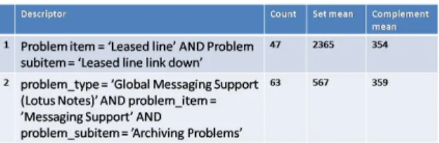
Treating the ST value as the performance measure for each ticket, the problem can be solved using the interesting subset discovery algorithm. Given a set A of problem columns, a subset of tickets characterised by a descriptor over A is expensive (i.e., interesting) if the ST characteristics of the subset are significantly worse than that of the set of
remaining tickets. Figure 4 shows some of the expensive
Figure 4. Expensive (Interesting) ticket types.
Figure 5. (a) Subsets of requests with very high response time. (b) Subsets of requests with very low response time.
significantly higher than the global ST average (360), as well as higher than the ST average values of their complement ticket sets, which justifies calling these ticket types as expensive. Note that the descriptors used different number of columns. The interesting subset discovery algorithm also discovered a number of ticket types which characterise
cheap problems i.e., problems whose ST characteristics
are significantly better than remaining tickets. Such cheap tickets indicate streamlined and efficient business processes and well-established and widely understood best practices for handling these tickets. Such cheap ticket types are useful for answering other kinds of business questions.
C. Transaction performance data of a data center
We next present another case study where we use the proposed interesting subset discovery algorithm on the performance data of various web service requests served by a data center. Today’s data centers consists of many servers hosting several applications. Each incoming requests is served by one or more applications hosted on the data center. Different Service Level Agreements (SLAs) are de-fined for the incoming requests to ensure high performance service. Most commonly defined SLAs are on the response time, e.g. an example SLA could be that each incoming request is served in less than 2s. Given such performance measures, the data center operators are very much interested in identifying poorly performing requests and finding their common properties. In this section, we present an example to demonstrate how the proposed interested subset discovery algorithm can provide interesting insights in this setup.
We present a case of transactional system, where a data center hosts the IT system of an on-line retail system. During on-line shopping clients perform various operations
such as browsing, comparison of items, shopping, redeeming of vouchers, etc. All these operations are performed in the form of one or more service requests. Each request received by the data center is associated with various at-tributes such as client IP address, Host name, date and
time of request, URL name, etc. The requested URL can
be further split to obtain derived attributes. For instance a URL http://abc.com/retail/AddToCart.jsp can be split to extract “http://abc.com”, “retail”, “AddToCart” and “jsp”. Similarly date and time of the request can be split to derive more attributes such as Day of the week, Date of the Month,
Month of the year, etc. Each request is associated with a
performance measure of response time. Thus, the database of requests can be observed as a set of records where each record consists of attributes and measures. Interesting subset discovery when applied on this data set provides insights into the subset of requests taking significanly different time than the rest of the requests. These insights can then be used to recommend fixes and make transformation plans.
Figure 5 presents some interesting subsets discovered on this data set. We ran interesting subset discovery algorithm to discover requests taking significantly more time as well as the requests taking significantly less time. Figure 5a presents the subsets of requests that take significantly more time than the rest of the requests. For instance, requests from U serId = U1 take significantly more time. There are 63 such requests and the average time taken by these requests is 2504.76ms. On the other hand, the average time taken by the rest of requests is 1107ms. Performing an impact analysis on this subset, we can derive that the impact factor of this subset is: 13042504..2976∗∗44863 = 0.27, where 448 is the total number of requests and 1304.29 is the average of all 448 requests. Thus a decrease of 10% in the response time of these 63 requests of this subset can result in a decrease of 2.7% in the overall service time.
Figure 5b presents the subsets of requests that take significantly less time than the rest of requests. In contrast to U serId = U1, we observed that U serId = U4 take significantly less time than the rest of the requests. There are 23 such requests with average time taken of 997ms whereas the average time taken by the rest of the requests is 1443ms. The data center operators use such insights to compare the subsets showing interestingly good and interestingly poor performance. Appropriate recommendations are then made such that per-user and per-organization service times can be improved.
D. Infrastructure data of an enterprise system
Figure 6. (a) Subsets with very high purchase price. (b) Subsets with very low purchase price.
information about cost and utilization. Enterprise system operators are very much interested in identifying properties of very expensive and very inexpensive servers. They are also interested in observing utilization of these machines and identifying heavily used servers and very unused servers. Such information is then used to make plans for server consolidation, purchasing new infrastructure, rebalancing the workload, etc.
Figure 6 presents the interesting subsets with respect to the purchase price. Figure 6a shows the subsets of machines with significantly higher purchase price than the rest of machines. This result gives insight into the expensive manufacturer, expensive sub-business, etc. For instance, the results show that machines with machinetype = server and category = T rade have an average price of USD 13335, whereas the average price of the rest of the machines is USD 3810. Performing an impact analysis on this subset, the impact factor of this subset is calculated as follows:
13335.24∗1439
9014.24∗2634 = 0.8, where total number of machines is 2634
and average price of these machines is 9014.24. Thus a 10% decrease in the price of the machines in this subset can result in an 8% decrease in the overall cost.
Another observation is as follows: Machines for sub business=SB1 are more expensive than rest of the machines (USD 35621 vs. USD 11970). On the other hand, as shown in Figure 6b, machines for sub-business SB2 are significantly less expensive than the rest of the machines (USD 1940 vs. USD 12732). Similar analysis can also be performed to identify highly used and unused machines by using resource utilization as a criteria.
These insights are then used to identify the high price machines, expensive sub-businesses, etc. and use this in-formation to make consolidation recommendations, perform cost-benefit analysis, and make transformation plans.
V. CONCLUSIONS AND FUTURE WORK
In this paper, we addressed the problem of discover-ing interestdiscover-ing subsets from a dataset where each record consists of various attributes and measures. We presented an algorithm to discover interesting subsets and presented
various heuristics to make the algorithm scale to large scale datasets without loosing interesting subsets. We presented a technique for performing impact analysis of the discovered interesting subset. We then presented four real-world case-studies from different domains of business processes and demonstrated the effectiveness of the interesting subset discovery algorithm in extracting useful insights from the datasets across diverse domains.
As part of future work, we plan to develop algorithms to perform root-cause analysis of the interesting subsets. The objective of root-cause analysis would be to find the cause of interestingness of a given subset. We also plan to systematically formulate and solve various scenarios of root cause analysis and impact analysis and perform their extensive experimental evaluation.
REFERENCES
[1] M. Atzmueller and F. Puppe, “Sd-map: a fast algorithm for exhaustive subgroup discovery,” in Proc. PKDD 2006, ser. LNAI, vol. 4213. Springer-Verlag, 2006, pp. 6 – 17.
[2] B. K. sek, N. L. c, and V. Jovanoski, “Apriori-sd: adapting association rule learning to subgroup discovery,” in Proc. 5th
Int. Symp. On Intelligent Data Analysis. Springer-Verlag, 2003, pp. 230 – 241.
[3] N. L. c, B. K. sek, P. Flach, and L. Todorovski, “Subgroup dis-covery with cn2-sd,” Journal of Machine Learning Research, vol. 5, pp. 153 – 188, 2004.
[4] N. L. c, B. Cestnik, D. Gemberger, and P. Flach, “Subgroup discovery with cn2-sd,” Machine Learning, vol. 57, pp. 115 – 143, 2004.
[5] J. Friedman and N. I. Fisher, “Bump hunting in high-dimensional data,” Statistics and Computing, vol. 9, pp. 123 – 143, 1999.
[6] M. Scholtz, “Sampling based sequential subgroup mining,” in
Proc. 11th SIG KDD, 2005, pp. 265 – 274.
[7] T. Scheffer and S. Wrobel, “Finding the most interesting patterns in a database quickly by using sequential sampling,”
Journal of Machine Learning Research, vol. 3, pp. 833 – 862,
2002.
[8] M. Natu and G. Palshikar, “Discovering interesting subsets using statistical analysis,” in Proc. 14th Int. Conf. on
Man-agement of Data (COMAD2008), G. Das, N. Sarda, and P. K.
Reddy, Eds. Allied Publishers, 2008, pp. 60–70.
[9] M. Atzmueller, F. Puppe, and H. Buscher, “Profiling ex-aminers using intelligent subgroup mining,” in Proc. 10th
Intl. Workshop on Intelligent Data Analysis in Medicine and Pharmacology (IDAMAP-2005), 2005, pp. 46 – 51.
[10] P. Clark and T. Niblett, “The CN2 induction algorithm,”
Machine Learning, vol. 3, no. 4, pp. 261–283, 1989.
[11] G. Palshikar, S. Deshpande, and S. Bhat, “Quest: Discovering insights from survey responses,” in Proc. 8th Australasian