Abstract—In Wireless Sensor Networks (WSN), maintaining a high coverage and extending the network lifetime are two conflicting crucial issues considered by real world service providers. In this paper, we consider the coverage optimization problem in WSN with three objectives to strike the balance between network lifetime and coverage. These include minimizing the energy consumption, maximizing the coverage rate and maximizing the equilibrium of energy consumption. Two improved hybrid multi-objective evolutionary algorithms, namely Hybrid-MOEA/D-I and Hybrid-MOEA/D-II, have been proposed. Based on the well-known MOEA/D algorithm, Hybrid-MOEA/D -I hybrids a genetic algorithm and a differential evolutionary algorithm to effectively optimize sub-problems of the multi-objec-tive optimization problem in WSN. By integrating a discrete particle swarm algorithm, we further enhance solutions generated by Hybrid-MOEA/D-I in a new Hybrid-MOEA/D-II algorithm. Simulation results show that the proposed Hybrid-MOEA/D-I and Hybrid-MOEA/D-II algorithms have a significantly better performance compared with existing algorithms in the literature in terms of all the objectives concerned.
Index Terms—Coverage optimization, MOEA/D, Multi-objective optimization, Wireless Sensor Networks.
I. INTRODUCTION
ireless Sensor Networks (WSNs) are self-organized networks consisting of sensor nodes capable of sensing, processing and wireless communication. Coverage control is a crucial issue in WSN, which mainly concerns how well a sensor network monitors a field with proper node deployment [1-3]. The energy of sensor nodes, network communication bandwidth and computing ability are generally limited resources, and thus the coverage sustainability in WSNs cannot always be guaranteed. How to balance the network energy consumption to prolong network lifetime while maintaining a high coverage rate is an important issue, which can be modeled as a multi-objective optimization problem (MOP) [4-5].
The goal to solve MOPs with two or more conflicting optimization objectives is to calculate an approximation of the
This work has been supported by the National Natural Science Foundation of China (No: 61202289).The Science and Technology Plan of Hunan Province (No. 2015GK3015).
Y. Xu is with College of Information Science and Engineering, Hunan University, Changsha 410082, China (Email: [email protected]).
O. Ding is with College of Information Science and Engineering, Hunan University, Changsha 410082, China (Email: [email protected]).
R. Qu, School of Computer Science, University of Nottingham, Nottingham NG8 1BB, U.K (Email: [email protected]).
K. Q. Li, Department of Computer Science State University of New York New Paltz, New York 12561, USA (Email: [email protected]).
Pareto Front. MOPs should be provided with multiple non dominated solutions concerning different objectives, which are difficult to be optimized if been converted into a single combined objective. Kulkarni et al. [6] used computational intelligence and evolutionary algorithms to solve MOPs of coverage control in WSN in complex and dynamic environments. Ozturk et al. [7] obtained better dynamic deployments for WSN by using an artificial bee colony algorithm. Kulkarni et al. [8] applied particle swarm optimization (PSO) to address issues such as optimal deployment, node localization, clustering, and data aggregation in WSN. It is shown that PSO is a simple, effective and efficient algorithm. Özdemir et al. [9] modeled the WSN coverage control problem as a MOP with two objectives: the coverage rate and the network lifetime. The multi-objective problem is then converted into a series of single objective sub-problems, each solved by a genetic algorithm. Experimental results showed that the proposed MOEA/D algorithm outperformed an improved non-dominated sorting genetic algorithm (NSGA-II) [10]. Shen et al. [11] proposed a MOEA/D-PSO algorithm by considering two optimization objectives including coverage rate and network lifetime, and applied a particle swarm optimization algorithm in MOEA/D. Since the balance of energy consumption has a great impact on the entire network, the energy equilibrium [12] is thus added as another objective in this research.
Hybrid algorithms and improved particle swarm optimizati-on algorithms have been well applied in other fields. Xu et al. [13] proposed a new hybrid evolutionary algorithm to solve multi-objective multicast routing problems in telecommunica-tion networks. The algorithm combines simulated annealing based strategies and a genetic local search to effectively find more non-dominated solutions. Experimental results demonstrated that both the simulated annealing based strategies and the genetic local search can efficiently identify high quality non-dominated solution sets for the problems and outperform other conventional multi-objective evolutionary algorithms. In a novel PSO algorithm based on the jumping PSO (JPSO) algorithm developed by Xu et al. [14], a path replacement operator has been used in particle moves to improve the positions of the particles with regard to the structure of the routing tree. The experimental results demonstrated the superior performance of the proposed JPSO algorithm over a number of other state-of-the-art approaches.
Based on our previous work, this paper considers the multi-objective coverage control optimization problem in WSN with three objectives, including the energy consumption, the coverage rate and the equilibrium of energy consumption, see
Hybrid MOEA/D Multi-objective Optimization Algorithms for WSN Coverage
Optimization
Ying Xu,
Member,
IEEE, Ou Ding, Rong Qu,
Senior Member,
IEEE
, Keqin Li,
IEEE Fellow
details in Section II. We propose two improved multi-objective algorithms, namely I and Hybrid-MOEA/D-II in Section IV. In order to diversify the search, two reproduction operators based on Genetic Algorithm (GA) and Differential Evolution (DE) have been hybridized in Hybrid-MOEA/D-I to obtain a better Pareto solution set. A weight is also set for each objective to guide the search direction. To further enhance the search ability of Hybrid-MOEA/D-I and preserve high quality individuals in each generation, a new Hybrid-MOEA/D-II algorithm is devised to integrate an improved discrete binary particle swarm optimization algorithm in [15] as the enhancement strategy to obtain a better Pareto solution set. An extensive set of experiments have been carried out in Section V to systematically investigate the performance of our proposed algorithms.
II. THEMULTI-OBJECTIVECOVERAGEOPTIMIZATION(MCO) PROBLEM
In WSN, coverage problems can be divided into face coverage, line coverage and target point coverage. In this paper, we use the target point coverage, refers to the target point at any time by one or more than one sensor node coverage. Assume the target field D is a two-dimensional square, the targeting point ST= {t1,t2,...,tM},tj= (xj, yj) are randomly distributed inD,
Mis the number of target points,j
[1,...,M],xjandyjare the coordinates of each target point. A set of sensor nodes S is randomly deployed over D where S{s1,s2,...,sn} ,) , , ( i i i i x y r
s ,nis the number of sensor nodes,
i
[
1
,...,
n
]
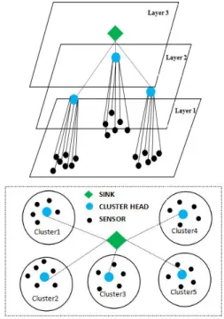
, ix and yiare the coordinates of each sensor node, and riis the maximum ideal sensing radius of sensor node si. We assume the Sink node has unlimited energy supply and each sensor node has the same physical structure, thus the communication ability, the initial energy and the computing power of each sensor node are the same. If the sensor node's energy is exhausted then this is not working, we call the node for the dead node. The Sink node or each sensor node can get its own location information and communicate with its neighboring nodes. In Fig. 1, randomly deployed sensor nodes (red nodes) and targeting points (blue nodes) are shown within a two-dimension square. The yellow point in the center is the
Fig. 1. Wireless Sensor Network with Random Node Deployment
Sink node. The coverage field of si at position (xi, yi) is indicated by the green circle area with a radius ofri.
A. The Network Model of WSN
In this paper, we adopt the well-known LEACH (Low Energy Adaptive Clustering Hierarchy) routing protocol for WSN as proposed by Heinzelman et al. [16]. In the LEACH clustered routing protocol using rounds to represent the network life. Each round begins with use the optimizer method to select the deployment solution, a set-up phase when the clusters are organized, followed by a steady-state phase when data are transfered from the nodes to the cluster head and on to the Sink node. The role of the cluster head node is to collect the information of the sensor nodes in the cluster, and then sends the data to the Sink node. The probability of each sensor node being selected as a cluster head ispc. Each non-cluster head node firstly calculates the energy consumption to communicate with all cluster heads, and then chooses its own cluster head with the lowest energy consumption. In order to balance the energy consumption, cluster head nodes are cyclically changed in each round based on a threshold valueH(i)[0,1] given by Eq. (1). If a randomly generated value is less thanH(i) then the node becomes the cluster head node in the current round.
otherwise G i if p r p
p i
H
0
) 1 mod ( 1 )
( (1)
pis the desired percentage of cluster head nodes in the sensor population, i represents the i-th node, r is the current round number, andGis the set of nodes that have not been selected as the cluster head in the last1/prounds.
targeting area with num clusters, where each cluster has Ks sensor nodes. Each sensor node can communicate directly with its cluster head. The middle layer is composed of all cluster heads, which can directly communicate with the Sink node at the top layer.
The Euclidean distance between sensor node si and the targeting pointtjat position (xj, yj) inDis:
2
2
(
)
)
(
)
,
(
s
it
jx
ix
jy
iy
jd
(2)The probability ofstbeing covered bysiis:
)
,
(
1
)
,
(
)
,
(
0
)
,
(
( , ) ) , ( j i e i i j i e i s s d r r r s s d j i i j it
s
d
r
r
r
t
s
d
r
r
e
t
s
d
r
t
s
p
i i te i t i (3)
Where re is the sensing error of a sensor node, ri is the maximum ideal sensing radius of a sensor node, and λ is the sensing attenuation coefficient. As long as the target pointtjis covered by at least one active sensor node, it is considered to be covered by the sensor network. Thus the probabilityptof the target pointstcovered by the network is defined as:
ni i j
t
p
s
t
p
1))
,
(
1
(
1
(4)B. The Definition of the Multi-objective Coverage Optimiza-tion (MCO) Problem
According to the characteristics of WSN, the LEACH clustered routing protocol is applied in this paper as described in Section 2.1. The essence of the MCO problem is to schedule the sensor node, that is, to select the appropriate node as the cluster head node, the active node and the inactive node, thus covering more target points, consume less energy and the energy of the whole network is more balanced.
In our proposed hybrid MOEA, the populationIP= {I1,I2, …,
Ipop} ofpopindividual solutionsIis defined in Eq. (5), each as a fixed-length chromosome of size equal to the total number of nodes in WSN. i
j
I is the j-th gene (sensor node) of the i-th individual or chromosome with a value of either -1, 0, 1 or 2, where -1 means a dead node, 0 represents an inactive node in
Sinactive, 1 means an active non-cluster-head node inSnonCH, and 2 represents a cluster-head node inSCH, respectively.E(sj) is the remaining energy of thej-th sensor node.
CH j j nonCH j j inactive j j j i j S s and s E if S s and s E if S s and s E if s E if I 0 ) ( 2 0 ) ( 1 0 ) ( 0 0 ) ( 1 (5)
}
....,
,1
{
}
,....,
1
{
pop
and
j
n
i
We set the population size pop as the same of the number of sub-problems N, each sub-problem composed of a weight
vector andmobjective functions. Take two objective functions as examples, in Fig .3. f1 andf2 are two objective functions,
F
are formulations of sub-problems,
[1,2,..,8].W={w1,...,w8} is the weight vector matrix, the sum of all elements of each row is 1, the number of rows is equal to the number of sub-problems, and the number of columns is equal to the number of objectives. The same definition can be found in [35].
The initial population is randomly generated. Each alive sensor node in the network becomes an active/inactive node
(a) Formula representation of sub-problems
(b) Graphical representation of sub-problems Fig. 3. An Example of Sub-problemslied field
with an equal probability (i.e.p= 0.5). An active node becomes a cluster-head (CH) node with the probability defined as follows:
))
1
mod
(
1
(
opt optopt
p
r
p
p
(6)The optimal selection probabilitypoptdefined in LEACH is calculated as:popt=Kopt/n, wherenis the number of nodes in the network, r is the current round number, and Kopt is the optimal number of constructed clusters,
765 . 02 2
n
Kopt , as
calculated in [16]. We define the following three objectives in our MCP in WSN.
1) The Energy Consumption
Energy consumption E(I) is the total energy consumed for transmitting, receiving, aggregating signals and activating sensors by solutionI, as defined in [17], formulation given in Eq. (7).
total num
i CH Sink DA
RX num
i scEsCH E E E E
I
E i
i
i
1 , 1 ,
) (
)
( (7)
Wherenum is the number of clusters,ciis thei-th cluster.
total number of nodes in the WSN. The allele of each gene can be either −1 to represent a dead node, 0 for an inactive node, 1 for a non-cluster-head nodes and 2 for a cluster-head node. Esi,sj is the energy consumption for transmitting data
from nodesitosj, which is defined in Eq. (8).
0 , , 4 0 , , 2 ,d
d
if
d
l
E
l
E
d
d
if
d
l
E
l
E
E
j S i j S i j S i j S i j i s s mp elec s s fs elec s s (8)Eelec is the energy consumed by the transceiver circuit, and Efs and Emp are the energy expenditures for transmitting
l-bit data to achieve an acceptable bit error rate, for the free space model and the multipath fading model [16], respectively. If the distance
j S i
s
d
, between two sensor nodes is less than the threshold d0 Efs/Emp , the free space model is applied, otherwise, the multipath model is used.ERXandEDA are the energy consumed for receiving and aggregating data computed as is defined in Eq. (9).
l
E
E
E
RX
DA
elec
(9)The total energy consumed for activating all nodes at the current round, namelyEtotal, is defined in Eq. (10).
n
i AC i
a E E
1
total * (10)
WhereEACis the energy consumed by activating an inactive node,aiindicates whether the sensor nodesiis active or not.
otherwise S s or S s if
a i nonCH i CH
i 10 (11)
2) The Coverage Rate
Coverage rate should be maintained to a high level in WSN. In this paper, we convert the problem of maximizing the coverage rate into minimizing the number of uncovered target pointsN(I).
M i t s U I N 1 ) ( ) ( (12) where otherwise 1 r ) s , d(s and S s if 0 sU( t) i active i t i (13)
U(st) is used to determine whether the target point st is covered.Mis the number of targeting points,Sactiveis the set of active sensor nodes.
3) The Energy Equilibrium
Definition 1: Regional energyThe monitoring area is divided into K grids, k[1,...,K]. The regional energy in thek-th grid
EQkequals to the average rest energy of all nodes in this grid.
k n i k k n E EQ k i
1 (14)
Wherenkis the number of nodes in thek-th grid, Eki is the rest energy of thei-th node in thek-th grid.
Definition 2: Energy Span The energy span in the current network (the equilibrium degree of energy consumption in the whole network) Es(I) can be represented by the ratio of the difference between the maximal and minimal regional energy to the maximum of the regional energy for solutionI.
) ( ) ( ) ( ) ( k k k EQ Max EQ Min EQ Max I
Es (15)
A smaller value ofEs(I) means the energy consumption in the network is more uniformly distributed.
Based on the definitions above, in order to achieve higher network coverage while effectively prolonging the network lifetime. we formally define the multi-objective coverage optimization problem of WSN with three objectives as follows:
1) f1(I)Minimize the number of uncovered targeting nodes
)) ( (
1 I Min N I
f )
( (16)
2) f2(I)Minimize the energy consumption of the network
))
(
(
2I
Min
E
I
f
(
)
(17)3) f3(I)Minimize the energy span
The third objective aims at preventing excessive energy consumption of sensor nodes in partial regions within the whole network as much as possible.
))
(
(
3I
Min
Es
I
f
(
)
(18)III. RELATEDWORK FOR THEMULTI-OBJECTIVECOVERAGE OPTIMIZATIONPROBLEM
In the literature, intensive research has been carried out on energy efficient routing protocols [18-23] and node placement [24-27] to reduce energy consumption for WSN. Early work often models the optimization problem with a single objective. Recently, the coverage optimization problem [28-34] in WSN has been modeled as a MOP. A MOP is composed of multiple conflicting objectives, and the performance improvement of one objective may cause the performance reduction of one or more other objectives.
Zhang et al. [35] proposed the MOEA/D algorithm by decomposing a MOP into a number of single objective optimization problems (i.e. sub-problems), and optimizing them simultaneously. By using the optimization information of the neighboring sub-problem, the sub-problem will be optimized. The Tchebycheff Approach is used as a decomposition method in MOEA/D due to its ability to transfer the objective function of the i-th sub-problem using non-convex Pareto optimal front as follows:
|}
)
(
|
{
max
*)
,
|
(
min
*1 j j
i j m i i
te
x
z
f
x
z
g
(19)where x denotes the decision variable space,
T i m i
i ( ,..., )
1
, 1,..., N denote a weight vector corresponding to thei-th sub-problem, j= 1, ...,m,
j 0 and 1,...,m1 , m is the number of objective functions,T m z z z* ( *,..., *)
1
weight vector
i is defined as a set of its several closest weight vectors in {1,2,...,N} .The neighborhood of the i-th subproblem consists of all the subproblems with the weight vectors from the neighborhood of
i .Özdemir et al. [9] used MOEA/D to solve the problem of multi-objective coverage optimization in WSN, which can provide a better performance than the classical NSGA-II algorithm. The differential evolution algorithm in Xu et al. [36] obtained a better performance than the classical NSGA-II algorithm on a two-objective coverage problem of WSN. Li et al. [37] proposed a multi-objective coverage optimization algorithm MOCADMA for WSN, which uses a memetic
algorithm with a dynamic local search strategy to optimize multiple objectives including the network coverage, the node utilization and the residual energy. The experiment and evaluation results show that MOCADMA have good capabilities in maintaining the sensing coverage, achieving higher network coverage, and effectively prolonging the network lifetime compared with some existing algorithms.
IV. THEPROPOSEDHYBRID-MOEA/D ALGORITHMS In this paper, we proposed a hybrid MOEA/D algorithm based on the work in [9], namely Hybrid-MOEA/D-I, by combining Genetic Algorithm (GA) and Differential Evolution (DE) as the mixed reproduction operator to optimize each sub-problem. To improve the efficiency of search, some of theNsub-problems are optimized by GA and the others by DE. Using the best solutions generated by Hybrid-MOEA/D-I as the initial solutions, an improved algorithm called Hybrid-MOEA/D-II is proposed to integrate a discrete binary particle swarm optimization (DPSO).
A. The Proposed Hybrid-MOEA/D-I Algorithm
To increase the population diversity, two different reproduction operators based on GA and DE have been designed in Hybrid-MOEA/D-I to optimize the N
sub-problems. The mutation probability of DE and GA operator is pmDE and pmGA, respectively. The crossover probability of DE and GA operator is pcrDE and pcrGA, respectively. For j [,12,. ,.m],fjis the value of the j-th objective function. We assume zjis the best value of thej-th objective function during the search, Ii is the current best solution for thei-th sub-problem in terms of all objectives, and
fj(Ii) is the value of the j-th objective function for Ii. IP (Internal Population) is the population maintained during the search.
The GA and DE operators will be selected randomly for solving each sub-problem. The procedure of the hybrid GA-DE operator used in Hybrid-MOEA/D-I, shown in Algorithm 1.
1) The DE reproduction operator
The DE operator includes three main procedures, i.e. the mutation, crossover and selection. Taking the l-th sub-problem as an example, the mutation operation of DE is as follows:
otherwise I
p rand I
I I
I h
r
mDE h
r u r l r r
) (
' (20)
Il is the solution of the l-th sub-problem which has T neighboring sub-problems. Iu andIh are two solutions of the
u-th and h-th neighboring sub-problems of Il, u and h are randomly selected indices from [1, 2, …, T]. I’ is the new solution generated from Il, Iu and Ih. l
r
I , u
r
I , Irh and
'
r
I represent the r-th gene ofIl,Iu,IhandI’, respectively, where
r
[1, …, n]. The real-value constant is a scaling factor. pmDE
(0, 1) is the mutation probability. The random numberrand
(0, 1).Algorithm 1 The framework of Hybrid-MOEA/D-I
Input:
•
N: the number of the sub-problems considered in MOEA/D;•
λ1,..., λN: a uniform spread ofNweight vectors;•
T: the number of the weight vectors in the neighborhood of each weight vector;•
genmax: the maximum number of generations; Output:•
Solution setIP= {I1,I2, …,Ipop} ,popis the size of population,here we setpop=N;
• Objec
tive function values for each solutionIiinIP:fj(Ii),i∈[1,…,pop],j∈[1,…,m]; Step 1 - Initialization
1.1:gen= 0; //genis the index of the current generation. 1.2: Divide the target area intoKgrids;
1.3: Randomly distributensensor nodes andMtarget points in the target area D;
1.4: Randomly generate an initial internal population,IPgen= {I1, I2, …,Ipop};
1.5: Initialize z = (z1,z2,…,zm),zj= min(fi,j), i[1,...,N],fi,jis
the value of thej-th objective for thei-th sub-problem; 1.6: Compute the Euclidean distances between any three weight
vectors and then work out theTclosest weight vectors to each weight vector;
1.7: For∀i = 1, 2,…,N, setB(i) = {i1,i2,…,iT}, which are the
index ofTclosest solutions to thei-th sub-problem; Step2 - Update:For i1,...,N
2.1: Reproduction:Randomly select three indicesl,uandh
fromB(i); 2.2: if rand<0.5 then
2.3: Generate a solutionI’fromIl,IuandIhby a mutation
operator with probabilitypmDEand then generateI’’with
probabilitypcrDEby the crossover operator;
2.4: else
2.5: Generate a solutionI’fromIlandIuby a crossover
operator with probabilitypcrGAand then generateI’’with
probabilitypmGAby a mutation operator;
2.6: end if
2.7: Updatez:j1,2,...,m, ifzj>fj(I’’), then setzj=fj(I’’); if gte(I’’|λl,z) ≤gte(Il|λl,z*), then setIl= I’’andF(Il) = F(I’’);
2.8: endFor Step3 - Stopping criteria
3.1:Ifgen==genmax thenstop and output {I1,I2, …,IN} and
{fj(I1),fj(I2), …,fj(IN)},j∈[1, …,m];
2
r
1
r
The polynomial crossover in Eq. (21) generates
)
,...,
,
(
" "2 '' 1 ''
n
I
I
I
I
fromI’andIl.pcrDE
(0, 1) is the crossover probability.
otherwise I
p rand I
I l
r
crDE r
r
'
" r[,1...,n] (21)
Fig. 4 shows a new offspring solutionI’’generated based on parents I’ and Il. A gene in I’’ is randomly selected from chromosomeI’and then other genes ofI’’are generated from eitherI’orIlbased on the crossover probabilitypcrDEdefined in Eq. (21).
Fig. 4. The Crossover Operation Procedure of DE
2) The GA reproduction operator
The GA operator includes three main procedures, i.e. the selection, crossover and mutation. Two individualsIlandIuare used to generate a new solutionIandI’based on a two-point crossover operation. To perform the mutation operation, a parent solution is randomly selected fromIorI’. AssumingI’
is selected, a new solution I’’ is generated based on the mutation operator as shown in Table I, where ''
r
I is the
r
-th gene of ( , ''.., ")2 '' 1 ''
n I I I
I andrand
(0, 1) is a random number. TABLE I THEMUTATIONOPERATOR OFGA''
r
I
0
'
r
I
'
1
r
I
'
2
r
I
rand
PmGArand> PmGA
rand
PmGArand> PmGA
rand
PmGArand> PmGA
1 2 0 2 0 1
Two reproduction operators DE and GA have been randomly selected to optimize all sub-problems, aiming to diversify the evolution to obtain high-quality solutions.
B. The Proposed Hybrid-MOEA/D-II Algorithm
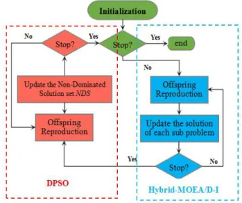
In Hybrid-MOEA/D-I, the weights of each sub-problem are fixed, so the search direction is determined. To further improve the efficiency of the search, an improved Discrete Particle Swarm Optimization (DPSO) algorithm is adopted as the enhancement strategy to Hybrid-MOEA/D-I, leading to a new hybrid algorithm Hybrid-MOEA/D-II. As shown in Fig. 5, Hybrid-MOEA/D-I algorithm is used to optimize the initial solutions generated randomly, and DPSO is applied to further enhance the search.
Taking five sub-problems in Fig. 6 as an example, the solution of each sub-problem is optimized by a randomly selected optimization operator to generate a new solution. Then, the current solution and the neighborhood solution (the solution of neighbor sub-problem) are updated. A DPSO is then applied to further enhance the search.
Fig. 5. The Hybridization of DPSO and Hybrid-MOEA/D-I
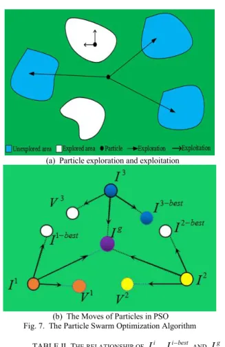
Particle swarm optimization (PSO) concerns two important issues: exploration and exploitation. Exploration is obtained by particles’ ability to change the original search trajectory to a new direction, i.e. to search the unexplored region in the search space. Exploitation is achieved by particles to search within the explored area. The relationship between exploration and exploitation is shown in Fig. 7(a). The velocity
Fig. 6. The Example of the Optimization Process of Hybrid-MOEA/D-II Algorithm
updating formula of discrete binary PSO algorithm proposed by Kennedy and Eberhart [38] is the same as that of the original PSO algorithm. Each individual is treated as a particle in thed
dimensional search space. For the MCP in WSN, the best previous position of thei-th particle
I
i
{
I
1i,
I
2i,
....
,
I
ni}
isrepresented as
I
ibest
{
I
1ibest,
I
2ibest,
...
,
I
nibest}
. The globalbest solution among all particles in the population is represented as
I
g
{
I
1g,
I
2g,
...,
I
ng}
. The position changevelocity for particleiis defined as
V
i
{
V
1i,
V
2i,
...,
V
ni}
. Eachparticle updates each bit i k
V
ofV
i according to Eq. (22). The moves of particles in DPSO are showed in Fig. 7(b).)
(
)
(
2 21
1 ki best ki kg ki
i k i
k
V
c
r
I
I
c
r
I
I
V
)
,...,
2
,1
(
n
k
(22)velocity formula is consists of three items, the first item i k
V
is the inertial part; the second itemc
1
r
1
(
I
kibest
I
ki)
isthe local cognitive part; and the third item
c
2
r
2
(
I
kg
I
ki)
isthe social cognitive part. In the improved DPSO, the value of i
k
I
, i best kI
and gk
I
can only be 0 or 1. Since only a few cluster head nodes exist in WSN, ik
I
seldom takes value 2, so we ignore the case for i
2
k
I
. In other words, the DPSO algorithm is used to schedule the active and non-active nodes in the case where the position and number of cluster heads are constant.
i
k best i
k
I
I
and
i
k g
k
I
I
take values of -1, 0 or 1, and the relationship of i bestk
I
, ik
I
and gk
I
is shown in Table II.(a) Particle exploration and exploitation
(b) The Moves of Particles in PSO Fig. 7. The Particle Swarm Optimization Algorithm
TABLE II THE RELATIONSHIP OF
I
ki ,I
kibest ANDI
kgvalue Possible values for i k
I , g k
I and ibest k
I How to change the value of i k
I
1 Ikibest orIkg is 1, and the value ofIki is
0.
i k
I needs to be changed to 1 with the most possibility. 0 IkibestorIkg is equal to the value ofIki. Iki should remain unchanged.
-1 Ikibestor g k
I is 0, and the value of i k
I is 1. Iki needs to be changed to 0
with the most possibility.
In other words, when i k
V
is 0, the value of the probability mapping function is 0; when ik
V
is less than 0 or greater than 0, the probability mapping function is an even function. When i kV
tends to be positive or negative infinity, the probability mapping function value is 1. The probability mapping function is defined in Eq. (23) as follows (see [12]):
0 1 ) exp( 1 2 0 ) exp( 1 2 1 ) ( i k i k i k i k i k V when V V when V V p (23)
When the velocity i k
V
is negative,(
i)
k
V
p
decreases; otherwise,(
i)
k
V
p
increases; if i kV
= 0,(
i)
k
V
p
is 0.The position of a particle is defined as: If i
0
k
V
otherwise
I
I
and
V
p
r
if
I
i k i k i k i k2
)
(
0
1If
V
ki
0
(24)
otherwise
I
I
and
V
p
r
if
I
i k i k i k 2 i k2
)
(
1
1r
andr
2 are randomly generated from the uniform distribution of interval[
0
,
1
]
.The pseudo code of Hybrid-MOEA/D-II is as shown in Algorithm2.
Algorithm 2 The framework of Hybrid-MOEA/D-II
Input:
•
The output of Hybrid-MOEA/D-IIP= {I1,I2, …,Ipop};•
genmax: the maximum number of generations; Output:•
The Non-Dominated Solution setNDS; Step 1 - Initialization1.1:Fori1,...,pop
1.2: Initialize the position of thei-th particleIi, thei-th
subproblem generated by Hybrid-MOEA/D-I. 1.3: The initial velocity of thei-th particle = 0; 1.4: end For
1.5: Updated the Non-Dominated Solution setNDS;
1.6: Choose the particle with the best objective function value of all the particles as the global best;
Step2 - Update:For i=1,...,N
2.1: Update the velocity of each particle according to Eq. (22) 2.2: Update the position of each particle according to Eq. (24); 2.3: Calculate the value of the objective function for each particle
based on the position of the particle; 2.4: Update the best and the global best;
2.5: Update the Non-Dominated Solution setNDS; 2.6:endFor
Step3 - Stopping criteria
3.1: Ifgen==genmaxthenstop and outputNDS;
3.2: elsegen=gen+ 1, go to Step2; 3.3: endIf
C. An Illustrative Example of the Proposed Hybrid Algorithms
compares the solutions found by Hybrid-MOEA/D-I (see Fig.8(a)) and Hybrid-MOEA/D-II (see Fig.8(b)) with the same random initial solution showed in Fig.8(a). For each solution, a black point represents a non-active node, a red point represents active non-cluster head nodes, and a green point indicates a
(a) A random initial solution,I
(f1(I)=0.0415J, f2(I)=2, f3(I)=0.0292)
(b) One optimal solution obtained by Hybrid-MOEA/D-I, I' ( ( ')
1 I
f =0.0200J, ( ') 2 I
f =0, ( ')
3 I
f =0.0280)
(c) One optimal solution obtained Hybrid-MOEA/D-II, I''
( ( '')
1 I
f =0.0177J, ( '')
2 I
f =0, ( '')
3 I
f =0.0280) Fig. 8. Comparison of Solutions found by Hybrid-MOEA/D-I and
Hybrid-MOEA/D-II
cluster-head node. X and Y represent the horizontal and the vertical coordinate, respectively. The values of the three objectives, i.e. f1(I) (the total energy consumption of each
round); f2(I) (the number of uncovered target points); f3(I) (the energy span), are shown below each solution.
For the random initial solutionI, the number of non-active nodes is 105, the number of non-cluster-head nodes is 85, and the number of cluster head nodes is 10. For the solution I'
obtained by Hybrid-MOEA/D-I , the number of non-active nodes is 156, the number of non-cluster-head nodes is 39, and the number of cluster-head nodes is 5. Comparing the two solutions I and I', we can see that the solution obtained by
Hybrid-MOEA/D-I has a better coverage (the uncovered node number ( ')
2 I
f = 0 < f2(I) = 2) with less energy consumption ( ( ')
1 I
f = 0.0200J < f1(I)= 0.0415J) and slightly better energy span ( ( ')
3 I
f = 0.0280 < f3(I) = 0.0292).
One non-dominated solution obtained by the DPSO enhancement strategy is Hybrid-MOEA/D-II is shown in Fig. 8 (c). The number of non-active nodes is 161, the number of non-cluster-head nodes is 34, and the number of cluster head nodes is 5. It can be seen that Hybrid-MOEA/D-II further enhances the search and obtains a better solutionI”with less energy ( ( '')
1 I
f =0.0177J < ( ')
1 I
f =0.0200J) compared with the
solution I’ generated by Hybrid-MOEA/D-I with the same coverage rate and energy span.
D. The Time Complexity Analysis
We firstly analyze the time complexity of MOEA/D-PSO in the literature [11] as follows. MOEA/D-PSO applied a PSO algorithm in MOEA/D to solve the coverage optimization problem in WSN with two optimization objectives including the coverage rate and the network lifetime.
1) The population size is N, i.e. N sub-problems, each sub-problem hasgnumber of iterations, each individual is represented as a fixed-length chromosome with size equal ton, i.e. the total number of nodes in WSN;
2) The GA operator: two point crossover and mutation operate on each gene in the chromosome, in the worst case, mutation and crossover operations need to be performed on
ngenes, requiringg×N×noperations;
3) The PSO operator: the main steps of PSO include updating the velocity, the position, the personal best and the global best, requiringg×N×n,g×N×n, g×Nandg×Noperations, respectively;
4) Each sub-problem updates the reference point and the neighborhood solutions, requiring g×N operations, respectively.
The time complexity of the MOEA/D-PSO algorithm is: O(MOEA/D-PSO)=g×(2×N×n+2×N×n+2×N+2×N)=4×g×
N×(n+1),
So the time complexity of MOEA/D-PSO is O(g×N×n). The basic idea of MOEA/D is to decompose a MOP into a set of single-objective optimization problems and optimize them simultaneously. We analyze the time complexity of Hybrid-MOEA/D-I as follows.
2) The DE operator is applied to half of the population, and is consists of the mutation and crossover operations. In the worst case,ngenes are applied mutation and crossover, so leading to 0.5×g×N×noperations, respectively;
3) The GA operator is applied to half of the population, which includes the crossover and mutation operations. In the worst case, this requires 0.5×g×N×nmutation and
crossover operations, respectively, applied to n genes; 4) Each solution of sub-problem needs to update reference
point and update the neighborhood solutions, leading tog
×Noperations, respectively;
The time complexity of the Hybrid-MOEA/D-I algorithm is O(Hybrid-MOE/D-I)=g×(2×0.5×N
×n+2×0.5×N×n+2×N)=2×g×N×(n+1), so its time complexity of Hybrid-MOE/D-I is O(g×N×n).
The main procedure of DPSO in Hybrid-MOEA/D-II is to update the particle velocity and particle position based on the solutions obtained by Hybrid-MOEA/D-I. The time complexity of Hybrid-MOEA/D-II is thus as follows.
1) The population size isN, i.eNparticles, each ofgiterations. Each individual has a fixed sizen.
2) According to the velocity and the position update formula in Eq. (23) and Eq. (25), the velocity and positon of each particle is updated. The length of the chromosome of each particle isn, so theseg×N×noperations, respectively; 3) To update the personal best of each particle and the global
best ,g×Nthese operations are required, respectively; The time complexity of Hybrid-MOEA/D-II is thus calculated as:
O(Hybrid-MOEA/D-II) =g× (2×n×N + 2×N)+ O(Hybrid-MOEA/D-I)= 4×g×N×(n+1).
Thus the time complexity of Hybrid-MOEA/D-II is O(g×N×n).
The above analysis indicates that the proposed Hybrid-MOEA/D-I and Hybrid-MOEA/D-II algorithms have the same time complexity as that of MOEA/D-PSO, showing that Hybrid-MOEA/D-I and Hybrid-MOEA/D-II can obtain better solutions without increasing the time complexity.
V. SIMULATIONRESULTS
In this paper, all algorithms are implemented using matlab. To evaluate the performance of Hybrid-MOEA/D-I and Hybrid-MOEA/D-II, simulation results are compared to those of MOPSO, NSGA-II, MOEA/D and MOEA/D-PSO using the same machine and parameters. The experimental parameters are shown in Table III.
A. Performance Evaluation of Different Algorithms
We compare the performance of our proposed two algorithms, i.e. Hybrid-MOEA/D-I and Hybrid-MOEA/D-II, with other four algorithms, including MOPSO, NSGA-II, MOEA/D and MOEAD-PSO for WSN with different number of sensor nodes (200, 300, 400 and 500 nodes, respectively). For each size of WSN, 10 topologies have been randomly generated and 20 independent runs have been repeated on each network topology.
We firstly compare the number of targets detected, the number of alive nodes and the remaining energy of each round. Each round includes a number of iterations of the algorithm (here we set the number of iterations as 20) to output the non-dominated solution set (NDS) and select a deployment
TABLE III PARAMETERS USED IN SIMULATIONS
Parameter Value Parameter Value
Network size:n
500Targe area 100m×100m
Number of grids 64
Number of target points 64 Maximum iterations
8000Maximum ideal sensing
radius:ri10m
Node initial energy:E0 0.02J The number of sub-problemsN 50
T 10
amp
0.0013pJ/bit/m4pcrGA 0.8
pmGA 0.03
pcrDE 0.9
pmDE 0.7
Eelec 50nJ/bit fs
100pJ/bit/m2EDA 5nJ/bit
0.5
c1 1
c2 2
solution. Then, we compare the coverage rate and energy consumption rate of different algorithms. We also compare the three objectives of NDS obtained by different algorithms. Moreover, to evaluate the solutions set of each algorithm, we used the Set Coverage metric (C-metric) [39] as the evaluation criteria. For two NDS sets A and B, C-metric is defined as:C(A,B)|bB|aA:ab/|B|, here b is a solution inB
and
a
is a solution inA. Note thatC(A,B)1C(B,A), andAis better thanB,ifC
(
A
,
B
)
is higher thanC(B,A)over many tests. C-metric calculates the fraction of solutions in the NDSobtained by one algorithm which are dominated by the NDS
obtained by another algorithm. Finally, we compare the running time and theNDSobtained at the tenth round of each algorithm.
B. The Comparison of Total Number Targets Detected
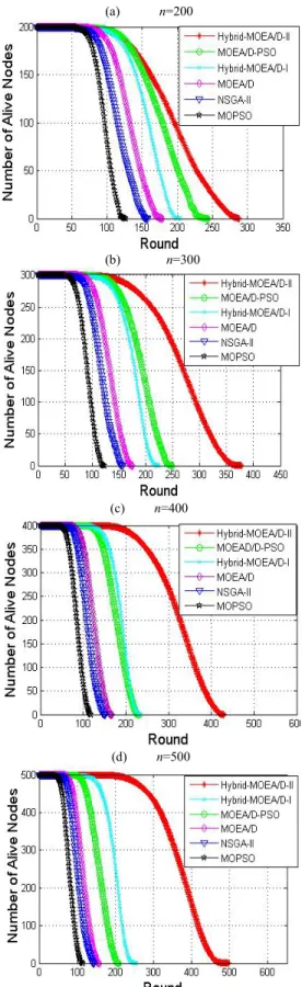
C. The Comparison of the Number of Alive Nodes
Fig. 10 compares the performance of all six algorithms in terms of the number of sensor nodes alive for WSN with different number of sensor nodes. Compared with other
(a) n=200
(b) n=300
(c) n=400
(d) n=500
Fig. 9. The comparison of total number targets detected
(a) n=200
(b) n=300
(c) n=400
(d) n=500
each round, prolonging network life time by saving more node energy.
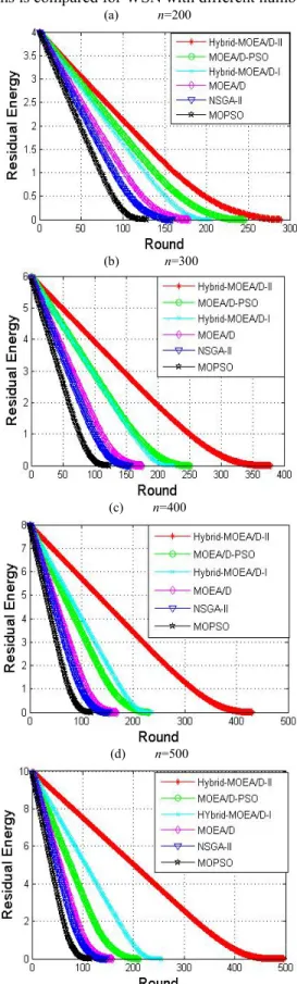
D. The Comparison of the Remaining Energy
In Fig. 11, the residual energy of sensor nodes of different algorithms is compared for WSN with different number of
(a) n=200
(b) n=300
(c) n=400
(d) n=500
Fig. 11. The comparison of residual energy
nodes. It shows again that more residual energy have been retained by Hybrid-MOEA/D-II for WSN during each round. This is clearer for WSN with more nodes.
(a) n=200
(b) n=300
(c) n=400
(d) n=500
E. The Comparison of Coverage rate and Energy Consumption rate
Fig. 12 compares the coverage rate and energy consumption of sensor nodes of six algorithms. Our proposed Hybrid-MOEA/D-II algorithm again has a higher coverage rate
(a) n=200
(b) n=300
(c) n=400
(d) n=500
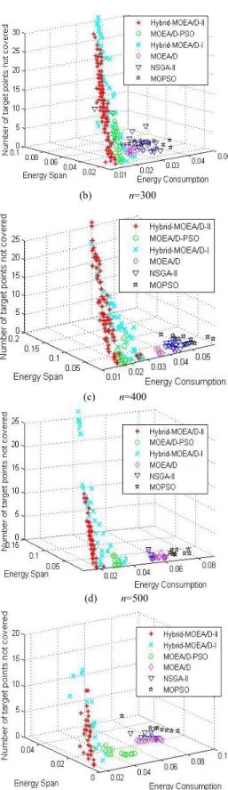
Fig. 13. The comparison of non-dominated solutions
and lower energy consumption rate for wireless sensor networks with different number of nodes.
F. The Comparison of Non-dominated Solution Sets
In Fig. 13, the non-dominated solution sets within the tenth rounds of six different algorithms are compared on WSN with different number of nodes. Hybrid-MOEA/D-I and Hybrid-MOEA/D-II perform better than other four algorithms by obtaining better Pareto fronts with respect to the three objectives defined in Section II. Better NDS sets have been obtained by Hybrid-MOEA/D-II compared with Hybrid-MOEA/D-I for four different sizes of WSN, which demonstrate the effectiveness of the DPSO enhancement strategy.
TABLE IV DOMINATION OFHYBRID-MOEA/D-I(I)VERSUSMOEA/D( II)
ANDNSGA-II( III)
n=200
round C(I,II) C(II,I) C(I,III) C(III,I)
1 1 0 1 0
25 1 0 1 0
50 0.66 0.06 1 0
75 0.625 0 0.7 0
100 0.75 0 0.9 0
125 0.667 0.111 0.16 0
n=300
round C(I,II) C(II,I) C(I,III) C(III,I)
1 1 0 1 0
25 1 0 1 0
50 1 0 1 0
75 1 0 1 0
100 1 0 1 0
125 0 0.051 0 0
n=400
round C(I,II) C(II,I) C(I,III) C(III,I)
1 1 0 1 0
25 1 0 1 0
50 1 0 1 0
75 1 0 1 0
100 1 0 1 0
125 0.5 0.4 0 0
n=500
round C(I,II) C(II,I) C(I,III) C(III,I)
1 1 0 1 0
25 1 0 1 0
50 1 0 1 0
75 1 0 1 0
100 1 0 1 0
G. The Comparison of Set Coverage Metric
Table IV and Table V compare C-metric of our proposed hybrid algorithms with MOEAD-PSO, MOEA/D and NSGA-II for WSN withn= 200, 300, 400 and 500 nodes in the network at each round.
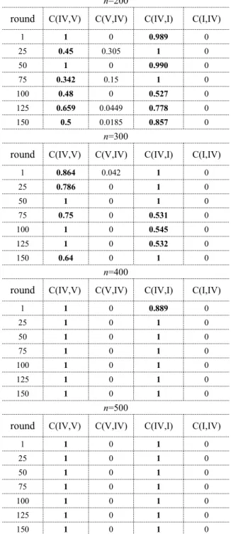
TABLE V DOMINATION OFHYBRID-MOEA/D-II( IV)VERSUS
MOEA/D-PSO( V)ANDHYBRID-MOEA/D-I( I )
n=200
round C(IV,V) C(V,IV) C(IV,I) C(I,IV)
1 1 0 0.989 0
25 0.45 0.305 1 0
50 1 0 0.990 0 75 0.342 0.15 1 0 100 0.48 0 0.527 0 125 0.659 0.0449 0.778 0
150 0.5 0.0185 0.857 0
n=300
round C(IV,V) C(V,IV) C(IV,I) C(I,IV)
1 0.864 0.042 1 0 25 0.786 0 1 0
50 1 0 1 0
75 0.75 0 0.531 0 100 1 0 0.545 0 125 1 0 0.532 0
150 0.64 0 1 0
n=400
round C(IV,V) C(V,IV) C(IV,I) C(I,IV)
1 1 0 0.889 0
25 1 0 1 0
50 1 0 1 0
75 1 0 1 0
100 1 0 1 0
125 1 0 1 0
150 1 0 1 0
n=500
round C(IV,V) C(V,IV) C(IV,I) C(I,IV)
1 1 0 1 0
25 1 0 1 0
50 1 0 1 0
75 1 0 1 0
100 1 0 1 0
125 1 0 1 0
150 1 0 1 0
Table IV presents the values of C-metric of three algorithms, i.e., Hybrid-MOEA/D-I, MOEA/D and NSGA-II. The Experi-ments show that all C-metric values of Hybrid-MOEA/D-I (I) are larger than the those of MOEA/D(II) and NSGA-II(III), which means Hybrid-MOEA/D-I has the best performance among the three algorithms. For example, forn= 200, at round = 25, all C(I, II) are larger than C(II, I), which means
non-dominated solutions generated by Hybrid-MOEA/-D-I dominate all those generated by MOEA/D. There is only one exception, forn= 300, at round 125, the C-metric value of C(I, II) is slightly larger than C(II, I). This means that the non-dominated solution set found by MOEA/D at this round has a better diversity than that of Hybrid-MOEA/D-I. However, from Figure 12(b), we can see that at round 125, the Coverage rate and Energy Consumption rate of Hybrid-MOEA/D-I are much better than those of MOEA/D.
Table V shows the comparison of the C-metric of Hybrid-MOEA/D-II, MOEA/D-PSO and Hybrid-MOEA/D-I with different network sizes at each round. For example, forn= 200, the non-dominated solutions generated by Hybrid-MOEA/D-II dominate 34.2% of those generated by MOEA/D-PSO at round 75, but the non-dominated solutions generated by MOEA/D-PSO algorithm dominate none of those by Hybrid-MOEA/D-II. When n becomes larger, Hybrid-MOEA / D-II obtains even better performance.
H. The Comparison of Running Time
In Table VI, the running time of these six algorithms is compared after 10 rounds. Although the running time of Hybrid-MOEA/D-II is slightly longer than the other algorithms, it always obtains much better results.
TABLEVI THE COMPARISON OF RUNNING TIME OF EACH ALGORITHM
n
Algorithm 200 300 400 500
Hybrid-MOEA/D-II 33.1s 48.4s 64.3s 79.6s
MOEA/D-PSO 27.1s 42.7s 53.8s 71.4s
Hybrid-MOEA/D-I 20.9s 30.8s 40.2s 50.6s
MOEA/D 17.5s 28.1s 34.8s 44.5s
NSGA-II 11.5s 15.8s 21.2s 26.5s
MOPSO 19.0s 28.4s 37.7s 49.4s
VI. CONCLUSION
The issues of reducing and balancing the energy consumption while retaining high coverage rate represent conflicting objectives for WSN. In this paper, we model the coverage control problem in WSN as a MOP by considering three objectives, including the coverage rate, the energy consumption and the energy consumption equilibrium. A Hybrid-MOEA/D-I algorithm has been proposed based on the well-known MOEA/D algorithm. To increase population diversity, hybrid GA and DE reproduction operators have been applied in Hybrid-MOEA/D-I. This shows Hybrid-MOEA/D-I achieves a higher quality solution than MOEA/D.
In Hybrid-MOEA/D-I, each objective is optimized by a randomly generated weight, and the search direction is thus determined with the fixed weights. To further enhance the search ability of Hybrid-MOEA/D-I and preserve high quality individuals in each generation, we propose a new Hybrid-MOEA/D-II algorithm by introducing a discrete binary particle swarm optimization algorithm (DPSO) as the enhancement strategy to obtain better Pareto solution set.
MOEA/D-PSO in the literature, and demonstrate that our proposed algorithms have a similar time complexity with that of MOEA/D-PSO.
Experimental results show that both the Hybrid-MOEA/D-I and Hybrid-MOEA/D-II perform significantly better than those of MOEA/D, NSGA - II, MOPSO and MOEA/D-PSO without increasing the time complexity. With DPSO as the further enhancement strategy, Hybrid-MOEA/D-II obtained much better performance than that of Hybrid-MOEA/D-I. The comparisons using the C-metric demonstrate that both the hybrid reproduction operator and the DPSO enhancement strategy have the ability to get better solution. . In our future work, we plan to apply learning strategies to further improve the performance of our proposed algorithms. In addition, we plan to consider the coverage problem of WSN within more complex real world scenarios, such as those with mobile charger nodes in the networks.
REFERENCES
[1] B. Wang, “Coverage Control in Sensor Networks,”in Springer, London, 2010.
[2] H. M. Ammari, “Coverage in Wireless Sensor Networks: A Survey,”
Network Protocols & Algorithms, vol. 2, no. 2, pp. 27-53, 2010.
[3] X.-x. Xiang, H.-G. Huang, and Y.-d. Li, “Hybrid sensor networks coverage-enhancing approach based on particle swarm optimization,”
Application Research of Computers, vol. 27, no. 6, pp. 2273-2275, 2010.
[4] J. Jia, J. Chen, G. Chang, Y. Wen, and J. Song, “Multi-objective optimization for coverage control in wireless sensor network with adjustable sensing radius,”Computers & Mathematics with Applications, vol. 57, no. 11-12, pp. 1767-1775, 2009.
[5] F. Fang and S. P. Chen, “Node deployment model of multi-objective optimization in wireless sensor networks,” Application Research of
Computers, vol. 32, no. 4, pp.1166-1168, 2015.
[6] R. V. Kulkarni, A. Förster, and G. K. Venayagamoorthy, “Computational Intelligence in Wireless Sensor Networks: A Survey,” IEEE
Communications Surveys & Tutorials, vol. 13, no. 1, pp. 68-96, 2011.
[7] C. Ozturk, D. Karaboga, and B. Gorkemli, “Probabilistic Dynamic Deployment of Wireless Sensor Networks by Artificial Bee Colony Algorithm,”Sensors, vol. 11, no. 11, pp. 6056-6065, 2011.
[8] R. V. Kulkarni, and G. K. Venayagamoorthy, “Particle Swarm Optimization in Wireless-Sensor Networks: A Brief Survey,” IEEE Transactions on
Systems Man & Cybernetics Part C, vol. 41, no. 2, pp. 262-267, 2011.
[9] S. Özdemir, B. A. A. Attea, and Ö. A. Khalil, “Multi-Objective Evolutionary Algorithm Based on Decomposition for Energy Efficient Coverage in Wireless Sensor Networks,” Wireless Personal
Communications, vol. 71, no. 1, pp. 195-215, 2013.
[10] K. Deb, A. Pratap, S. Agarwal, and T. Meyarivan, “A fast and elitist multiobjective genetic algorithm: NSGA-II,” IEEE Transactions on
Evolutionary Computation, vol. 6, no. 2, pp. 182-197, 2002.
[11] X. Shen, J. Li, and Q. Zhang, “WSN coverage hierarchical optimization method based on the improved MOEA/D,” Metallurgical & Mining
Industry, vol. 7, no. 6, pp. 348-354, 2015.
[12] T. Liang, H. Zhou, J. Xie, and K. Wang, “Multi-objective coverage control strategy for wireless sensor networks,” Chinese Journal of Sensors &
Actuators, vol. 23, no. 7, pp. 994-999, 2010.
[13] Y. Xu, R. Qu, and R. Li, “A simulated annealing based genetic local search algorithm for multi-objective multicast routing problems,”Annals of
Operations Research, vol. 206, no. 1, pp. 527-555, 2013.
[14] R. Qu, Y. Xu, J. P. Castro, and D. Landa-Silva, “Particle swarm optimization for the Steiner tree in graph and delay-constrained multicast routing problems,” Journal of Heuristics, vol. 19, no. 2, pp. 317-342, 2013.
[15] J. H. Liu, R. H. Yang, and S. H. Sun, “The analysis of binary particle swarm optimization,”Journal of Nanjing University, vol. 162, no. 47, pp. 17-33, 2011.
[16] W. B. Heinzelman, A. P. Chandrakasan, and H. Balakrishnan, “An Application Specific Protocol Architecture for Wireless Microsensor
Networks,”IEEE Transactions on Wireless Communications, vol. 1, no 4,pp. 660--670, October. 2002.
[17] E. A. Khalil, and B. A. A. Attea, “Energy-aware evolutionary routing protocol for dynamic clustering of wireless sensor networks,”Swarm &
Evolutionary Computation, vol. 1, no. 4, pp. 195-203, 2011.
[18] A. Gupta, A. Thakur, H. S. Saini, R. Kumar, and N. Kumar, “H-IECBR: HBO based-Improved Energy Efficient Chain Based Routing protocol in WSN,” in IEEE International Conference on Power Electronics, New Delhi, India, 2016, pp. 1-4.
[19] B. Kushal, and M. Chitra, “Cluster based routing protocol to prolong network lifetime through mobile sink in WSN,” IEEE International
Conference on Recent Trends in Electronics, pp. 1287-1291, 2016.
[20] Y. Li, P. Wang, R. Luo, and H. Yang, “Reliable energy-aware routing protocol for heterogeneous WSN based on beaconing,”in International
Conference on Advanced Communication Technology, Pyeongchang,
Korea, 2014, pp. 109-112.
[21] C. Del-Valle-Soto, C. Mex-Perera, A. Orozco-Lugo, and G. M. Galvan-Tejada, “An efficient Multi-Parent Hierarchical routing protocol for WSNs,”in Wireless Telecommunications Symposium, Washington, DC, 2014 , pp. 1-8.
[22] Y. S. B. Kaebeh, S. S. Tyagi, M. K. Soni, and M. E. E. Omid, “SAERP: An energy efficiency Real-time Routing protocol in WSNs,”in International
Conference on Optimization Reliabilty and Information Technology,
Faridabad, India, 2014, pp. 249-254.
[23] S. Rani, J. Malhotra, and R. Talwar, “Energy efficient chain based cooperative routing protocol for WSN,”Applied Soft Computing, vol. 35, no. C, pp. 386-397, 2015.
[24] M. Elsersy, M. H. Ahmed, T. M. Elfouly and A . Abdaoui, “Multi-objective sensor placement using the effective independence model (SPEM) for wireless sensor networks in structural health monitoring,” in Wireless Communications and Mobile Computing
Conference,Dubrovnik,2015, pp. 576-580.
[25] H. Idoudi and J Bennaceur, "Fault tolerant placement strategy for WSN."in IEEE Wireless Communications and Networking Conference, Doha, Qatar, 2016, pp. 1-6.
[26]V. Sharma, R. Patel, H. Bhadauria, and D. Prasad, “NADS: Neighbor Assisted Deployment Scheme for Optimal Placement of Sensor Nodes to Achieve Blanket Coverage in Wireless Sensor Network,” Wireless
Personal Communications, vol. 90, no. 4, pp. 1903-1933, 2016.
[27] J. Guo and H. Jafarkhani, “Sensor Deployment With Limited Communication Range in Homogeneous and Heterogeneous Wireless Sensor Networks,”in IEEE Transactions on Wireless Communications, vol. 15, no. 10, pp. 6771-6784, Oct. 2016.
[28] J. Xu, F. L. Ning and D. W. Jiang, "The analysis and research of Wireless Sensor Network coverage optimization algorithm," in International
Conference on Automatic Control and Artificial Intelligence (ACAI 2012),
Xiamen, China, 2012, pp. 2052-2055.
[29] P. P. Das, N. Chakraborty and S. M. Allayear, "Optimal coverage of Wireless Sensor Network using Termite Colony Optimization Algorithm,"
in International Conference on Electrical Engineering and Information
Communication Technology (ICEEICT), Dhaka, Bengal, 2015, pp. 1-6.
[30] C.-P. Chen, S. C. Mukhopadhyay, C.-L. Chuang, T.-S. Lin, M.-S. Liao, Y.-C. Wang, and J.-A. Jiang, “A hybrid memetic framework for coverage optimization in wireless sensor networks,” IEEE transactions on
cybernetics, vol. 45, no. 10, pp. 2309-2322, 2015.
[31] E. Kaffashi, M. T. Shoorabi and S. H. Bojnourdi, “Coverage optimization in wireless sensor networks,”in International Conference on Computer and
Knowledge Engineering (ICCKE), Mashhad, Iran, 2014, pp. 322-327.
[32] H. I. Sweidan and T. C. Havens, “Coverage optimization in a terrain-aware wireless sensor network,”in IEEE Congress on Evolutionary Computation
(CEC), Vancouver, BC, 2016, pp. 3687-3694.
[33] M. Sharawi, E. Emary, I. A. Saroit and H. El-Mahdy, "WSN's energy-aware coverage preserving optimization model based on multi-objective bat algorithm," in IEEE Congress on Evolutionary
Computation (CEC), Sendai, Japan, 2015, pp. 472-479.
[34] H. P. Gupta, and S. Rao, “Demand-based coverage and connectivity-preserving routing in wireless sensor networks,” IEEE
Systems Journal, vol. 10, no. 4, pp. 1380-1389, 2016.
[35] Q. Zhang, and H. Li, “MOEA/D: A Multiobjective Evolutionary Algorithm Based on Decomposition,”IEEE Transactions on Evolutionary
Computation, vol. 11, no. 6, pp. 712-731, 2007.
[36] Y. L. Xu , X. H. Wang and H. Zhang, “Improved differential evolution to solve the two-objective coverage problem of wireless sensor networks,”in
Chinese Control and Decision Conference (CCDC), Yinchuan, China,
[37] Z. Chen, S. Li, and W. Yue, “Memetic algorithm-based multi-objective coverage optimization for wireless sensor networks,”Sensors, vol. 14, no. 11, pp. 20500-20518, 2014.
[38] J. Kennedy, and R. Eberhart, "Particle swarm optimization." IEEE
International Conference on Neural Networks, vol.4, pp. 1942-1948, 1995.
[39] R. Rajagopalan, C. K. Mohan, P. Varshney, and K. Mehrotra, "Multi-objective mobile agent routing in wireless sensor networks." in
IEEE Congress on Evolutionary Computation, 2005, pp. 1730-1737.
Ying Xu Ph.D, Associate Professor
obtained her Ph.D degree from the University of Nottingham in UK in March 2011. She is currently an associate professor in the College of Information Science and Engineering at Hunan University of China. Her research focuses on Artificial Intelligence, Multi-objective Optimization and Machine Learning techniques for solving some real world optimization problems, including wireless sensor networks, network routing, etc.
Ou Dingreceived his Bachelor’s degree in
electronic information engineering from Wenhua College in Huazhong University of Science and Technology in 2014. He is currently pursuing the master degree in the field of Multi-objective Optimization for Wireless Sensor Networks from College of Information Science and Engineering, Hunan University.
Rong Qu(SM’12) received the Ph.D degree
in Computer Science from the University of Nottingham,Nottingham, U.K., in 2002.
She is currently an Associate Professor in the School of Computer Science, University of Nottingham. Her research interests include meta-heuristics,constraint program-ming, mathematical programprogram-ming, case based reasoning and knowledge discovery techniques on scheduling, especially educational timetabling, healthcare personnel scheduling and network routing problems, and a range of combination optimization problems including portfolio optimization.
Keqin Li(SM’96) is a SUNY Distinguished
Professor of computer science. He is an Intellectual Ventures endowed visiting chair professor at Tsinghua University, China. His research interests are mainly in design and analysis of algorithms, parallel and distributed computing, and computer networking. He has over 285 refereed research publications.
Professor Li is currently or has served on the editorial board of the IEEE TRANSACTIONS ON PARALLEL AND
DISTRIBUTED SYSTEMS, IEEE TRANSACTIONSON
COMPUTERS, Journal of Parallel and Distributed Computing, International Journal of Parallel, Emergent and Distributed Systems, International Journal of High Performance