Local hull based surface construction of volumetric data from silhouettes

University of Warwick institutional repository: http://go.warwick.ac.uk/wrap

This paper is made available online in accordance with

publisher policies. Please scroll down to view the document

itself. Please refer to the repository record for this item and our

policy information available from the repository home page for

further information.

To see the final version of this paper please visit the publisher’s website.

Access to the published version may require a subscription.

Author(s): Dongjoe Shin and Tjahjadi, T.

Article Title: Multi-user indoor optical wireless communication system

channel control using a genetic algorithm

Year of publication: 2008

Link to published article:

http://dx.doi.org/10.1109/TIP.2008.926149

Publisher statement: “© 2008 IEEE. Personal use of this material is

permitted. Permission from IEEE must be obtained for all other uses, in

any current or future media, including reprinting/republishing this

material for advertising or promotional purposes, creating new

Local Hull-Based Surface Construction

of Volumetric Data from Silhouettes

Dongjoe Shin, Student Member, IEEE and Tardi Tjahjadi, Senior Member, IEEE

Abstract

The Marching Cube (MC) is a general method which can construct a surface of an object from its volumetric data generated

using a shape from silhouette method. Although MC is efficient and straightforward to implement, a MC surface may have

discontinuity even though the volumetric data is continuous. This is because surface construction is more sensitive to image noise

than the construction of volumetric data. To address this problem, we propose a surface construction algorithm which aggregates

local surfaces constructed by the 3D convex hull algorithm. Thus, the proposed method initially classifies local convexities from

imperfect MC vertices based on sliced volumetric data. Experimental results show that continuous surfaces are obtained from

imperfect silhouette images of both convex and non-convex objects.

Index Terms

Shape from Silhouettes, Marching Cube, Delaunay triangulation, Surface extraction

I. INTRODUCTION

T

HE 3-dimensional (3D) visual hull is generated by the intersection of multiple 3D cones that are created by backprojection of 2D silhouettes of different views of an object onto 3D space [1]. Approaches to object reconstruction involving 3D hull are collectively called Shape from Silhouette (SfS) techniques [2] and an octree is the most widely used representation to describe a visual hull. The construction of an octree involves projecting an initial bounding cube (which encloses an object in 3D space) onto multiple images of the object taken at different views, and splitting the cube into eight smaller cubes called octants if the projection intersects a silhouette [3]. These octants are then classified as one of three cases: outside, inside and intersection. Thus, object reconstruction is achieved by carving out octants classified as outside, and surfaces are extracted from the resulting octree for an effective visualisation.

The Marching Cube (MC) is the most successful method for surface construction from an octree [4]. It estimates surface triangles from intersection octants, and the location of the triangles are determined by the configuration of inside vertices of an intersection octant. However, the MC generated surface may contain unexpected holes or discontinuities that are not present in its octree. One reason for surface discontinuity is due to the connectivity of octants as was first reported by Mercier and Meneveaux [5] who also proposed a process which thickens the intersection octants to ensure 6-connectivity, and changes an inside octant to an intersection octant. But the process is not straightforward to implement for the following reasons: since it checks whether two adjacent inside and outside octants are in the same hierarchy level of the octree, the octree hierarchy is repeatedly referred to when creating a surface; and the subsequent image pixel based refining method has to verify whether two adjacent surface lines remain connected.

Manuscript received February xx, 2007. This work was partially supported by Tardi Tjahjadi Publications.

Another possible reason for discontinuity is due to the topological ambiguity of the MC algorithm. For example, when a face of an octant has an intersection point with a surface in each of its four edges, the topologically correct connection among the intersection points becomes ambiguous and this results in Type A hole problem [6], [7], and Chen et al. reported seven ambiguous configurations that create holes and incorrect connectivity [8].

A more practical reason for surface holes is due to erroneous camera calibration and imperfect silhouettes, which change the position of the projection of an octant or the value at the projection position. Therefore, traditional octree construction methods take special care of these processes. Szeliski used adaptive thresholding followed by a local shrinking operation for silhouette detection, and a hexagonal calibration pattern is attached to the turntable for a precise camera calibration at every rotation [9]. Mercier and Meneveaux used over-exposed images and a seed-fill algorithm to generate silhouette images and attach an LED on the rotational axis of the turntable for accurate calibration [5]. However, measurement error is inevitable in calibration and there are no image preprocessing algorithms that can deal with all effects of imaging conditions. For example, a seed-fill algorithm can reduce noise on silhouette images but at the expense of losing concave surface details.

On the other hand, octree construction is robust against image noise because an octant is not removed when nonzero-valued pixels are found within the projection of the octant. Thus, despite some unpredictable error on silhouette images, the resulting octree can be similar to the octree created from error-free silhouette images if the size of an octant is not too small. The octree construction only changes the status of an octant from inside to intersection. Therefore, to retain non-convex surface details in silhouette images, simple thresholding is preferable for its octree construction. However, in this case, its MC surface is significantly degraded.

Thus, we propose a surface construction method for an imperfect MC result. The method exploits the connectivity information of an octree, which is referred when building a new face from imperfect MC vertices. We premise a general non-convex object as a piecewise convex set, and an object surface is constructed from an aggregate of its local convex surfaces. The initial MC vertices are grouped into different slices and classified, and connections are made with appropriate vertices in adjacent slices in order to determine local convex regions. The Bayes rule is used for classifying and connecting the MC vertices. The conditional probability density functions (pdfs) used by the Bayes rule are estimated from octree vertices that are regarded as sampled points on the true 3D object.

A similar method which uses data slices for surface generation has also been proposed in [10]. However, the cylindrical mapping of this method focuses on merging 3D range data obtained from different views and only a simple object is considered. The principal axis of such an object must pass through the object, and a normal of the principal axis must pass through only one point on the object, i.e., the object is convex. An alternative mapping procedure is also proposed for a more complex object, e.g., an object with a single cavity like a cup. Nevertheless, the algorithm has not been designed for a general object. Thus, if there are multiple clusters in a slice then the algorithm will have difficulty in aligning the slices.

II. SURFACE FROM SILHOUETTES

A. Obtaining an octree from silhouettes

A major process of octree construction is the projection of an octant and an intersection test to determine if the projection intersects a silhouette. However it is cumbersome to estimate every projection matrix at a particular position from known camera motion such as pure rotation, pure translation or planar motion which consists of both rotation and translation in the plane. For these motions, projection matrices are normally derived from the projection matrix at the reference position.

A projection matrix can be decomposed into two matrices whose elements are related to the internal and external camera parameters [11]. For example, for a point in 3D space represented by a vector~x3d, its projection~x2d is

~x2d=K[R ~t]~x3d, (1)

whereK is a matrix related to the internal camera parameters.R and~tare rotation and translation in 3D space, respectively, and are determined by the external camera parameters. Hence, the projection matrix is P =K[R ~t].

If the same camera is used for grabbing all images without changing its internal parameters, then K is the same for all projection matrices. Also, if the camera motion is assumed to be a circular motion consisting of pure rotation on the same plane, e.g., as in a turntable image sequence, the projection matrix in (1) is parmeterised by a rotation angle, i.e.,

P(θ) =K



   

cosθ sinθ 0 tx −sinθ cosθ 0 ty

0 0 1 0



   

, (2)

where θ is a rotational angle from the reference position, and tx andty respectively represent thex andy translation when

θ= 0. In most cases,P(θ) in (2) is acceptable butθ is not always accurately measured and the rotational axis is wobbly at times. These errors propagate to the surface construction.

A silhouette is generated by thresholding an image during an intersection test. Any error in the resulting silhouette is insignificant as far as constructing an octree is concerned because the intersection test only determines an octant with intersection status and not the position of the internal vertices. However, the resulting error in surface construction is significant since the locations of inside vertices are crucial in defining the iso-surface of an octant. For example, when the backprojection of an octant results in one vertex within a silhouette, i.e., case a, the octant is classified as intersection and the inside vertex is easily identified. However, it is ambiguous to identify an inside vertex when only part of the edge of an octant is within a silhouette (case b) or the silhouette is entirely within an octant (case c), although the projection of the octant is classified as intersection. Case b and c are frequently found when imperfect silhouette images and projection matrices are used or when the octree resolution is not small enough.

B. Marching cube and its variants

Consider a 3D vertex point~x3d with a cost function

ci(θi, ~x3d) =   

 

1 if P(θi)~x3d∈ Si

0 otherwise

, (3)

where Si is an object silhouette in i-th image and θi is i-th rotational angle from the reference. The point is classified as outside when

n Y

i=0

ci(θi, ~x3d) = 0, (4) wherenis the total number of silhouette images. Therefore, if any projection of a 3D vertex is erroneously classified as outside a silhouette, it supersedes other statuses previously defined in other silhouettes. This erroneous classification often occurs if there is noise in the silhouette and no inside vertices are found even though the octant is classified as intersection, e.g., as in case b and c. Thus, the MC surface loses surface patches that result in holes and unattached object segments. To avoid this situation, the Voting MC (VMC) counts the number of cases classified as outside and identifies an outside vertex if the vote is greater than a thresholdvth [14]. Thus, the decision function (4) is revised as

n X

i=0

ci(θi, ~x3d)−vth≤0, 0≤vth< n. (5) The problem with VMC is that its result varies with the threshold level even for a convex object, and it is difficult to choose an appropriate threshold.

C. Delaunay triangulation and convex hull

An alternative approach, the 3D Delaunay Triangulation (DT) [15], constructs a surface by defining tetrahedrons from arbitrarily distributed 3D points. The 3D DT characterises each tetrahedron by not allowing any point within its circumsphere. If there is such a point then DT subdivides the tetrahedron without changing the shape of a super tetrahedron [16]. The Constrained Delaunay Triangulation (CDT) [17] has been evolved in order to include a predescribed boundary. In 3D however, CDT cannot tetrahedralise some special ployhedron without an additional point or surface modification, e.g., a twisted prism, and the problem in determining whether a given polyhedron can be tetrahedralised is NP-complete [18].

Although other variations of the DT algorithms, e.g., conforming constrained DT [19] and the conforming DT [20], have been proposed to solve the problem, they assume that initial boundary information is given. Besides, the result of DT in 3D is not triangles but tetrahedrons, i.e., three additional faces are redundantly created in order to make one surface triangle.

DT is topologically related to a convex hull. If for a set of points I in the n-dimensional space, a set of the pointsI′ _are

fitted to a hyper quadric inn+1dimension, e.g.,x2_+y2_+z2_=d2_{forn= 2, then the projection of the convex hull ofI}′ _onto

< L ocalconv ex classification >

R

econ stru ction im ages

In itial M C surface

O

ctree con stru ction

C

lu sterin g on each slice

C

alibration at referen ce p osition

oth er projection m atrices estim ation

B

in ary im ages

Texture m ap an d m app in g p o sition

L o calconv ex v ertices tab le

is it 1:n or n :1

C

alibration im age

p df cub es estim ation

3D C

onv ex H u ll

D

iv ide a clu ster an d m ak e n 1:1

A

ccum u lation local su rface

<

3D

H u llb ased surface gen eration >

n o y e s

T

ree tab le gen eration

<

I

n itiald ata prep aration >

Fig. 1. The overall surface construction process.

III. OVERVIEW OF THE PROPOSED METHOD

The overall surface construction process is illustrated in Fig. 1 where the proposed method involves the processes enclosed in two grey-shaded processing boxes, i.e., the local convex classification and 3D hull based surface generation. The projection matrix estimation determines the projection matrix at the reference position and uses it to estimate other projection matrices in the circular motion. In our experiment the rotational angleθis set to 6 degree. Images of an object are thresholded to generate silhouette images, and sixty projection matrices, one for each of the sixty image planes are fed to the initial data preparation process.

An octree data is first constructed in the initial data preparation process and it is used to estimate the initial MC vertices that are normally obtained from the best VMC. In our octree construction a 2D intersection test is used, i.e., an octant is backprojected onto every silhouette image, and if it intersects a silhouette the octant is classified as intersection and split into 8 suboctants. For robust octree construction, the backprojecion of an octant is approximated as a rectangle, and if the rectangle has no intersections then the corresponding octant is classified as background and is removed. There are numerous algorithms that facilitate the intersection test in 2D image planes. Szeliski proposed an almost real-time algorithm which uses a half distance transform [9]. Potmesil approximated the projection as a rectangle [22]. Chien and Aggarwal used a quad tree [23]. Ahuja and Veenstra reduced the number of silhouette images by only using orthographic views [24]. A few 3D intersection test algorithms have also been proposed in [25], [26]. However, since the speed of creating the volumetric data is not an issue in our research, the fundamental octree construction method has been developed for our surface construction process.

The proposed local-hull based surface estimation comprises two sequential processing blocks: local convex classification and 3D hull based surface construction. The first block determines local convex regions from the initial MC surface vertices. Data slicing and classification are required to define these convex regions. For the classification of initial vertices, cluster conditional pdfs are estimated from every octree slice. As a result of the first block, a tree table storing information on the cluster connection and local convex vertices table are passed to the next block.

IV. LOCAL HULL-BASED SURFACE CONSTRUCTION

Two properties of a 3D object are premised. The first is connectivity which assumes the surface of an object should cover an object tightly without any unattached object segment. If a surface is obtained without violating the first property, each edge of the surface should be traversed twice to make two connected patches. Otherwise there is a hole in the surface and the edge is called a dangling edge.

The second property due to the assumption of piecewise convexity of a 3D object is the continuity of an object. It allows a shape with local convexity to be similar to its adjacent convexity if they are connected [27]. To make this property more robust, an object needs to be sliced infinitesimally. However, each slice cannot be smaller than the size of the smallest octant. The second property enables the data distribution between two octree slices to be approximated. It considers a local convexity to be continuously connected to other local convexities in adjacent slices.

A. Volumetric data slicing

The proposed algorithm uses the best VMC vertices since they are closer to the actual surface than vertices of intersection octants, and the number of vertices are considerably reduced. On the other hand, the octree vertices are used to define a local convexity from MC vertices and their connections. In order to represent an object as a piecewise convex set, the data is sliced along the zaxis and the slicing interval is defined by the height of the smallest octant. Even though a MC surface has twice finer resolution, the same slicing level is used to keep the correspondence between an octree and a MC slice. The sliced results are stored in planes called MC slicesSmc_{. The corresponding octree vertices also need to be sliced and the results are stored} in octree slicesSoc_.

For a 3D delta function

δ(x, y, z) =

  

 

1 ifx=y=z= 0 0 otherwise

, (6)

the i-th sliced data of an octree (i.e.,Soc=∪iSioc(m, n)) is

Sioc(m, n) =o(x, y, z)δ(x−mT, y−nT, z−iT), (7) wherei,mandnare integer-valued indices andT is the slicing interval. The functiono(·)indicates whether an octant contains a 3D point (x, y, z), i.e.,o(x, y, z)is 1 if it is and 0 otherwise.

An interesting observation of a sliced octree data is that every four points in a sliceSoc

i are from the same octant. To treat these points equally, the index of the octree Soc _{needs to be quantised to give thei-th quantised octree slice}

Siocq[u, v] =

1

Y

j,k=0

Sioc(u+j, v+k). (8)

Hence, S_iocq[u, v]can be visualised on a binary image plane where a nonzero point represents an octant.

On the other hand, to represent MC data by the same slice index even though its sampling period is half of T, a binary image plane S_imcq[u, v] is only set to 1 when a MC vertex is found within uT ≤x < (u+ 1)T, vT ≤y <(v+ 1)T and

iT ≤z <(i+ 1)T. Thus, whilst the volume of nonzero points inS_iocq isT3_{, the volume of nonzero points at[u, v] in the}

quantised MC slice is bounded by

T3

8 ≤f(S

mcq

i [u, v])≤

7T3

where f(·)is a function which estimates the volume of nonzero points in the quantised MC slice. The actual volume of an objectvobj is smaller than the volume of MC slices, and which is smaller than the volume of the octree slices, i.e.,

vobj < X

i,u,v

f(S_imcq[u, v]) +T3(S_iocq[u, v]

− Simcq[u, v]S ocq

i [u, v])}< X

i,u,v

Siocq[u, v]T3 .

(10)

In practice, however, the volume of MC slices often violate (10) because the erroneous classification of octree vertices fails to correctly locate MC vertices.

Another observation from a sliced octree data is that each quantised octree slice of a non-convex object can have multiple clusters that are linked 8-neighbouring points on the quantised octree slice. These multiple clusters need to be connected to other clusters in adjacent slices to define a local convexity. The clustering in a quantised octree slice is trivial because points belonging to the same cluster are conglomerated in accordance with the presence of internal octants. Thus, identifying a cluster in S_iocq is simply a search for connected nonzero points among 8 neighbours. However, clustering in Smcq _{is not similarly} straightforward. A decision on the clustering and connecting of clusters in S_imcq is based on the Bayesian decision making rule [28] and a priori information of the decision is obtained fromS_iocq.

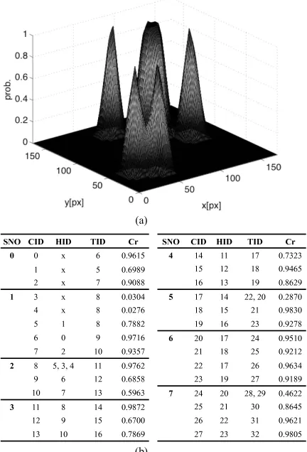
An octree of a dummy is illustrated in Fig. 2(a). The octree is obtained from 7 levels of octree construction from a 40[cm]x40[cm]x40[cm] initial octant, i.e., the smallest size of octant is 0.625[cm] and a total of 29 quantised octree slices and 60 clusters are found. Some slices of the octree,Smcq_i , are illustrated in Fig. 2(b) and each nonzero pixel in a slice indicates an octant, and octants belonging to the same cluster identification (ID) have identical grey value. For example, the slice 11 is forz = 6.875[cm], which is at shoulder height of the dummy.

B. Identifying a local convexity

A local convexity is identified by two processes: clustering onSmcq _{and connecting clusters between slices. Given a cluster} conditional pdf p(~t|ci)which gives the probability of a test data~tbelonging to a class ci, the problem of clustering is solved by searching for the maximum probability.

A probability mass function ofj-th cluster ini-th quantised octree slicePi(cj)is defined by the number ofj-th cluster data

nj and the total number of nonzero pointsnk, i.e.,

Pi(cj) = Pnj k=0nk

. (11)

Thus, the sum of cluster probabilities in a slice, i.e., P

j=0Pi(cj), is 1. From this a priori knowledge a cluster ID is predicted

when a nonzero point is found in Simcq. For example, if two clusters are found inS ocq

i and their probability arePi(c0) = 0.7

andPi(c1) = 0.3 then a nonzero point inSimcq is classified as clusterc0.

If points in j-th cluster are known to be more likely to be in a certain part of a slice, then the first a priori knowledge is enhanced by combining it with a second a priori knowledge obtained from the distribution of cluster data. If~t= [u v]T

represents the 2D position of a clustered data ini-th slice, a joint pdf of two random variables~tandcj that are not independent is

pi(~t, cj) =pi(~t|cj)Pi(cj) =pi(cj|~t)Pi(~t). (12) The a priori knowledge in (12) is converted to a test data conditional pdf of a clusterpi(cj|~t)called a posteriori pdf,

pi(cj|~t) =

pi(~t|cj)Pi(cj) P

jpi(~t|cj)Pi(cj)

(a)

(b )

Fig. 2. (a) 3D octree of a dummy from [27], which is sliced according to itsz_{value. (b) Examples of slices where each slice is quantised as 28x28 grid}

and a nonzero value on a slice represents an octant.

Therefore, in order to cluster MC vertices based on the Bayesian rule, pi(~t|cj)in (13) needs to be estimated.

Without any assumption on pi(~t|cj), a cluster conditional pdf of a test data~t= [u v] is estimated using the Parzen non-parametric density estimator [28] fromS_iocq. If the density function is known, the probabilityP thatj-th cluster data is found in a square with areawn centred at (x, y)is

P =

y+wn/2

X

v=y−wn/2

x+wn/2

X

u=x−wn/2

pi(~t|cj). (14)

In practice, the only information available is that nj data are classified as j-th cluster in Siocq. Thus, the probability thatk data fall within the square is P ≃k/nj, and the ratiok/nj converges to the trueP as the number of samples is increased.

The Parzen estimator increases the number of samples in a square by interpolating between samples in a window, i.e.,

pi(~t|cj) =

1

nj nj

X

i=0

wherew(·)is the Gaussian window with an area equals town. Since the size of a Gaussian window confines the range of the Gaussian function, the degree of smoothness of the pdf is determined bywn.

Each Siocq is used to estimate cluster conditional pdfs and those in the same slice are stored in a pdf cube. Therefore, a cluster decision function d(~t) which determines a cluster ID of a test data~t= [u v]T _{in thei-th quantised MC slice is}

d(~t) = max

j

pi(~t|cj)Pi(cj) , (16)

wherej represents a cluster ID in thei-th slice. Fig. 3(a) illustrates the construction of a pdf cube using (15) from the slice 8 shown in Fig. 2(b) where 5 clusters are shown in different grey shades.

Note that the cluster conditional pdf’s of connected clusters are similar because the second property assumes that the connected clusters have a similar shape. Thus, a decision function for connecting a clustercid on the current slicei needs to refer to the pdf cube in the next slice, i.e.,

e(cid, i) = max j {

X

~t∈cid

pi+1(~t|cj)Pi+1(cj)}. (17) The connection between clusters is summarised in a tree table, where a node of the tree represents a cluster and it stores information of bidirectional connection, i.e., a connected tail ID and head cluster ID (see Fig. 3(b)). A part of the tree table of the octree in Fig. 2(a) is shown in Fig. 3(b). Each row of the tree table shows a cluster ID (CID), the slice number (SNO), head and tail cluster ID (HID, TID). ‘x’ indicates that there are no connections, e.g., if HID is ‘x’ then a new local convexity starts from the current slice. On the other hand, a local convexity terminates the connection if a TID is ‘x’. Since it is assumed that there are no unattached clusters in an object, a cluster should not have ‘x’ as both of its head and tail ID. A slice with multiple clusters indicates that the object has non-convex shape and the resulting tree table has multiple HID’s or TID’s. To show similarity of connected clusters, a Cr column is added in the table. It is defined by the modulus of the approximated correlation coefficient between CID and TID’s. For example, the Cr of two clusterscmandcn in adjacent slices is estimated by

g(cm, cn) =

(P

ipj(~ti|cm)pj+1(~ti|cn))2 P

ip2j+1(~ti|cn)Pip2j(~ti|cm)

, (18)

wherecm is them-th cluster in the current slice andcn is then-th cluster, which is found as the TID ofcmin the next slice. When a current cluster has multiple tails then an average Cr value is used.

C. Local surface construction

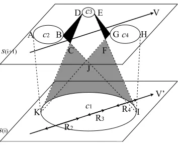
A local convexity is defined by two connected clusters in different slices. If the data is sliced reasonably small and every slice has a single cluster, the 3D hull algorithm will construct a good surface of a local convexity because the connected clusters are regarded as convex. However, if an object is not convex, a local convexity can have multiple connections (see Fig. 4). This means that the local convexity does not correspond to a convex shape since a convex shape is only possible with 1:1 cluster connection. Thus, the 3D hull algorithm will smooth some details of the object.

Fig. 4 shows an example of multiple connections. A cluster c1 in sliceSi is connected to three clusters c2,c3 and c4 in

(a)

(b )

SN O C ID H ID T ID C r 4 14 11 17 0.7323

15 12 18 0.9465 16 13 19 0.8629 5 17 14 22,20 0.2870 18 15 21 0.9830 19 16 23 0.9278 6 20 17 24 0.95 10 2 1 18 25 0.92 12 22 17 26 0.9634 23 19 27 0.9189 7 24 20 28,29 0.4622 25 2 1 30 0.8645 26 22 31 0.9621 27 23 32 0.9805 SN O C ID H ID T ID C r

[image:11.612.198.414.54.372.2]

0 0 x 6 0.96 15 1 x 5 0.6989 2 x 7 0.9088 1 3 x 8 0.0304 4 x 8 0.0276 5 1 8 0.7882 6 0 9 0.97 16 7 2 10 0.9357 2 8 5,3,4 11 0.9762 9 6 12 0.6858 10 7 13 0.5963 3 11 8 14 0.9872 12 9 15 0.6700 13 10 16 0.7869

Fig. 3. (a) A 3D pdf cube contains every cluster conditional pdf found in a quantised MC slice. A cluster conditional pdf interpolates 170x170 pixels and

the size of the Gaussian window is 5. (b) Part of the tree table from the slice 4 to 7 shown in Fig. 2(b).

algorithm to the multiple connections in Fig. 4 results in a local surface connecting A, B, D, E, G, H, I and K. This causes black areas to be added and they smooth some details of the object.

However, if the multiple connections are simply treated as multiple 1:1 cases, then connections betweenc1 andc2, between c1 andc3, and betweenc1 andc4 unnecessarily duplicate the surface in the grey area enclosed by K, C, J, F and I in Fig. 4.

To address this problem the proposed method divides multiple connections inton1:1 connections with an appropriate division so as to minimise possible duplication of surface patches in the common area. For example, c1 in Fig. 4 is divided into 3

subclusters to make three 1:1 connections.

The division is performed along the best representative vector of the multiple clusters which is estimated by an eigen analysis. If~tij = [u v]T representsi-th point in clusterj,mdata points in the n-th branched cluster areX =

h

~t11 ~t21 · · · ~tmn i

and the covariance matrix C of the data is C = P j

P

i ~tij−m~ ~tij−m~

T

, where m~ is the mean of X. If there are orthonormal column vectors~ei, the projection of the matrixC onto the orthonormal vectors is

C[~e1~e2] = [~e1~e2]





λ1 0

0 λ2



, (19)

where λi is the eigen value of the eigen vector~ei ofC.X is also represented by a weighted sum of the eigen vectors, i.e.,

X = [e~1e~2] [e~1e~2]TX= [e~1e~2]X′. These eigen vectors are used as orthonormal basis to express~tij, and the eigen vector corresponding to the maximum eigen value of C is the best vector which represents X, e.g., if λ1 > λ2 then~e1 is the best

A B

C

D E

F

G H

I

J

K c 1

c 2

c 3

c 4

s(i+ 1)

s (i

)

R

2

R

3

R

4

V

V ’

Fig. 4. 1:n_{branching case. If the 3D hull algorithm is simply applied to multiple connections, some object details will be smoothed. To avoid the smoothing,}

the clusterc1is divided into 3 subregions,R2,R3 andR4on the projection of the eigen vectorV′and n 1:1 connections are made.

Once the best eigen vector of the multiple clusters is found, each column vector of X is projected onto ~e1 to find the

distribution of clusters on the eigen vector, i.e., a location of~tij on the eigen vector~e1 is lij =~tijT~e1. Thus, the minimum

and maximum locations ofj-th cluster,(lmin, lmax)j, indicate the distribution ofj-th cluster. To divide a cluster into multiple subclusters, the data distributions are normalised. Finally, the cluster to be divided is projected onto~e1 and divided according

to the normalised cluster distributions. In Fig. 4, the eigen vector of the three clusters are represented as V in S(i+ 1). The projection of V onto S(i), V’, is used to divide the three clusters and the dividing ranges are denoted byR2,R3 andR4.

V. EXPERIMENTAL RESULTS

The proposed algorithm has been evaluated on four objects with shapes of different complexities as shown in the first row of Fig. 5. The oil burner (Fig. 5(a)) has four non-convex details in its sides. The dragon (Fig. 5(b)) has a more complex shape than Fig. 5(a) with numerous merged or branching clusters in its slices. The bust (Fig. 5(c)) has only one cluster in every slice but it is not convex. Finally, the vase has the simplest shape.

Each image of an object is captured as a 640x480 colour image and from the 60 images of each test object, an 8-level octree was constructed (see second row of Fig. 5). For an appropriate silhouette detection, thresholding is performed after Gaussian smoothing and contrast enhancement. A seed-fill operation [5] is then applied to minimise silhouette detection errors. When an object has non-convex details as shown in Fig. 5(a) and (b), any remaining errors are manually removed after the seed-fill operation. A projection matrix at the reference position is estimated by a linear SVD method from a 3D calibration rig with 2.45438[pixel] re-projection error.

The MC surfaces of the four test objects are shown in the last row of Fig. 5. Since the MC results are obtained from small silhouette and projection error, MC triangles are correctly constructed from most intersection octants. However, some sharp details, e.g., tail of the dragon, are partly removed because of the resolution of the octant, i.e., the tail of the dragon is too sharp when compared to the current octree resolution, resulting in case b or c intersection.

[image:12.612.223.400.52.196.2]

(a) (b ) (c) (d)

(e) (f) (g) (h )

[image:13.612.185.429.54.353.2]

(i) (j) (k ) (l)

Fig. 5. 8-level octrees and MC surfaces of four test objects: (a)-(d) Images of objects at the reference position; (e)-(h) The corresponding octrees respectively

with 362320, 75504, 267072 and 378448 octants; (i)-(l) MC surfaces from (e)-(h).

(a) (b) (c) (d)

(e) (f) (g) (h )

(i) (j) (k) (l)

Fig. 6. (a)-(d) Silhouette images with 10% noise added; (e)-(f) MC surfaces estimated from silhouette images with 5% noise added; (i)-(l) the best VMC

[image:13.612.185.430.407.701.2]

100 95 90 85 80

0

0.1 0.2 0.3 0.4 0.5 0.6 0.7 0.8 0.9

1

vote [% ] lo s t o c t. / t o t. o c t.

0 5 10 15 20

0

0.1 0.2 0.3 0.4 0.5 0.6 0.7 0.8 0.9

1

noise[% ] lo s t o c t. / to t o c t.

bur ne

r

drag on bu st v a se

(a)

[image:14.612.217.396.50.342.2]

(b)

Fig. 7. (a) Lost octants ratios using MC for varying noise ratios. (b) Lost octants ratios using VMC for varying voting thresholds.

octants ratio is almost nil. However, when a small amount of noise is added to the silhouette images, a significant number of octants do not result in a surface. Examples of MC surfaces when 5% noise is added are shown in Fig. 6(e)-(h).

VMC can address the noise sensitivity of MC. It can reduce the number of lost octants with an appropriate voting threshold. Fig. 7(b) shows the lost octants ratio of two data sets containing the four test objects. The first set is corrupted with 10% noise and the VMC results are denoted by solid lines. The second set is corrupted with 15% noise and the VMC results are denoted by dashed lines. The voting threshold which gives the best performance is referred to as the best voting threshold. The best voting threshold for the first set is about 90%, but when more noise is added a smaller voting threshold becomes appropriate to minimise the lost octants ratio. However, too small a voting threshold increases the lost octants ratio. This is because as the voting threshold becomes smaller it is possible to have an intersection octant with 8 inside corners. This particular case is regarded as an inside octant by MC and no surface is constructed.

The best VMC results from images with 10% noise added are shown in Fig. 6(i)-(l). As illustrated, VMC can minimise the lost octants but the results are degraded when compared to the ideal MC results, e.g., the surfaces are not continuous. Thus, the best VMC result may include sufficient surface vertices but the surface connection is not always correct.

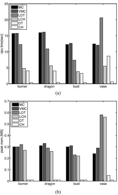
When a simple convex hull (CH) algorithm is applied to the best VMC result, many shape details are lost (see Fig. 8(a)-(d)) whilst the results of applying the proposed method shown in Fig. 8(e)-(g) preserve them. However, when the object is totally convex (Fig. 8(d)), CH is the best in terms of processing time, memory usage and approximation efficiency. To show the approximation efficiency for varying noise ratios, the total number of surface triangles on the reconstructed burner using 6 methods are summarised in Table 1, where LDT and LCH represent local DT and local CH, respectively. LDT which uses DT algorithm for constructing local convex hull is developed to show the efficiency of the proposed method, LCH.

(a) (b) (c) (d )

(e) (f) (g ) (h)

Fig. 8. Surface reconstruction from the best VMC result: (a)-(d) using the convex hull algorithm; (e)-(h): using the proposed method.

TABLE I

NUMBER OF SURFACE TRIANGLES ON RECONSTRUCTED BURNER FOR VARYING NOISE RATIOS.

0% 5% 10% 15% 20%

MC 14271 5640 296 124 24

VMCa 14271 43069 44489 44622 45520

DT 160048 541476 575812 58540 601980

CH 410 434 388 430 410

LDT 245112 850428 915312 918676 949672

LCH 3662 4380 4566 4538 4426

a_{obtained from the best VMC with voting threshold from 100% to 80%}

best VMC. Thus, the number of surface triangles constructed by these methods does not change significantly even after noise addition. CH approximates shape with the smallest number of triangles but the quality of the visual appearance of the result depends on the shape of objects. DT constructs similar surfaces to CH but the number of triangles are significantly increased because DT forms tetrahedrons from every four 3D points. Therefore, LDT results in the largest number of triangles because it performs DT between every two slices. On the other hand, LCH is the second most efficient method, but unlike CH it is able to construct non-convex details.

The performance of the proposed method (LCH) in terms of the required CPU time and peak memory usage is compared with 5 surface construction algorithms: MC, VMC, CH, DT and LDT. Qhull code is used for the implementation of CH and DT [29], and LCH and LDT also incorporate Qhull code. A look up table for the 256 possible cases of surface construction [4] is provided for MC to avoid rotational and complementary symmetry checking, which is known to be the most time consuming process in MC. In general, CH requires the shortest time, followed by DT, LCH, LDT, VMC and MC (see Fig. 9(a)). In the case where DT constructs a large number of tetrahedrons for the vase, DT is slower than LCH.

burner dragon bust vase 0 5 10 15 20 25 c p u t im e [s e c ] M C VM C LD T LC H D T C H

burner dragon bust vase

0

0.1 0.2 0.3 0.4 0.5 0.6 0.7

p e a k m e m. [ M B ] M C V M C LDT LCH D T C H

(a)

[image:16.612.213.402.49.361.2]

(b )

Fig. 9. (a) CPU time and (b) peak memory usage required by 6 algorithms to construct 4 objects.

of clusters. The proposed method also needs to incorporate the Qhull algorithm with complexityO(nlnv)[21].

The last experiment is performed on a dummy which can move its limbs and makes arbitrary non-convex shapes. Some examples of 60 input images are shown in Fig. 10(a)-(c). When only a simple thresholding process is applied, the silhouette images include detection errors as illustrated in Fig. 10(d)-(f). For examples, the right leg in Fig. 10(d) has shrunk and the left arm in Fig. 10(e) has unexpected noise because of shading effect. Furthermore, although the images of the right arm does not have significant noise, the contour of the arm are altered in all its silhouette images, and as a result most parts of the right arm vanish in its MC surface. Nonetheless, a 7-level octree with 30[cm] as the initial octant size (Fig. 10(g)) results in an acceptable 3D reconstruction. But the results using MC and 90% VMC have many unattached segments and holes (see Fig. 10(h) and (i)). LCH produces the best continuous surface (Fig. 10(j)).

VI. CONCLUSION

A surface constructed from 3D volumetric data facilitates the rendering of the object. In this paper we explore a method which constructs triangular patches from an octree, and a robust construction is achieved by assuming two properties of a 3D object. The connectivity property presumes a surface covers all area of an object tightly without unattached object segments. The continuity property assumes an object as piecewise convex and a local convexity is similar in shape to the adjacent convexity if they are connected.

(a) (b) (c)

(d) (e) (f)

[image:17.612.182.434.50.348.2]

(g) (h) (i) (j)

Fig. 10. (a)-(c) A dummy with different poses. (d)-(f) The corresponding silhouette images using simple thresholding. (g) 7-level octree. (h) MC surface.

(i) 90% VMC surface. (j) LCH surface.

slices by the Bayesian decision making rule in order to define local convexities. Finally, a convex hull algorithm creates local surfaces which are combined to complete the surface construction.

The experimental results show that LCH produces quality surfaces with good performance. Its approximation efficiency is better than those produced by other algorithms, e.g., MC, VMC, DT and LDT, requiring a reasonable CPU time. However, its peak memory usage is higher than CH and DT because the method needs to store local connection data. Also, any concavity in the xy plane may disappear in LCH, i.e., the concavity of a cluster in a slice is regarded as a 2D convex. This problem can be alleviated by dividing a 2D non-convex cluster into convex regions - it is like a 2D version of LCH. Another issue of the proposed method is the quality of the triangular patches, i.e., elongated or thin patches are caused by using a small slicing level and the convex hull algorithm. However, it can be improved by inserting refining points on the side of the thin triangles.

REFERENCES

[1] A. Laurentini, “The visual hull concept for silhouette-based image understanding,” IEEE Trans. Pattern Anal. Mach. Intell., vol. 16, no. 2, pp. 150–162,

1994.

[2] E. Trucco and A. Verri, Introductory Techniques for 3D Computer Vision, 1st ed., New Jersey: Prentice Hall, 1998.

[3] T. H. Hong and M. O. Shneier, “Describing a robot’s workspace using a sequence of views from a moving camera,” IEEE Trans. Pattern Anal. Mach.

Intell., vol. 7, no. 6, pp. 721–726, 1985.

[4] W. E. Lorensen and H. E. Cline, “Marching cubes: A high resolution 3D surface reconstruction algorithm,” Comput. Graphics, vol. 21, no. 4, pp. 163–169,

1987.

[5] B. Mercier and D. Meneveaux, “Shape from silhouette: Image pixels for marching cubes,” in Proc. 13th Int. Conf. Central Europe on Computer Graphics,

Visualization and Computer Vision (Journal of WSCG’05), 2005, vol. 13, pp. 112–118.

[6] C. Zhou, R. Shu and M. S. Kankanhalli, “Handling small features in isosurface generation using marching cubes,” Comput. Graph., vol. 18, no. 1, pp.

[7] K. S. Delibasis, G. K. Matsopoulos, N. A. Mouravliansky and K. S. Nikita, “A novel and efficient impelementation of the marching cubes algorithm,”

Comput. Med. Imag. Grap., vol. 25, pp. 343–352, 2001.

[8] N. Chen, L. Serra and H. Ng, “Surface extraction: Dividing voxels,” in Proc. 18th Int. Congress and Exhibition Computer Assisted Radiology and

Surgery, 2004, vol. 1268, pp. 225–230.

[9] R. Szeliski, “Rapid octree construction from image sequence,” Compt. Vis. Graph. Image Process., vol. 58, no. 1, pp. 23–32, 1993.

[10] I. R. Khan, M. Okuda and S. Takahashi, “Regular 3D mesh reconstruction based on cylindrical mapping,” in Proc. 2004 IEEE Int. Conf. on Multimedia

and Expo(ICME 2004), 2004, pp. 133–136.

[11] R. Hartley and A. Zisserman, Multiple View Geometry, 1st ed. Cambridge: Cambridge University Press, 2000.

[12] R. Y. Raj Shekhar, E. Fayyad and J. F. Cornhil, “Octree based decimation of marching cubes surfaces,” in Proc. Visualization 1996, 1996, pp. 335–342,

499.

[13] L. P. Kobbelt, M. Botsch, U. Schwanecke and H. P. Seidel, “Feature-sensitive surface extraction from volume data,” in Proc. SIGGRAPH 2001, 2001,

pp. 57–66.

[14] Y. Yemez and F. Schmitt, “3D reconstruction of real objects with high resolution shape and texture,” Image Vision Comput., vol. 22, no, 13, pp. 1137–1153,

2004.

[15] F. Aurenhammer, “Voronoi diagram - a survey of a fundamental geometric data structure,” ACM Comput. Surv., vol. 23, no. 3, pp. 345–405,1991.

[16] A. Bowyer, “Computing dirichlet tessellations,” Comput. J., vol. 24, no. 2, pp. 162–166, 1981.

[17] L. P. Chew, “Constrained delaunay triangulations,” Algorithmica, vol. 4, no. 1, pp. 97–108, 1989.

[18] J. Ruppert and R. Seidel, “On the difficulty of triangulating three dimensional nonconvex polyhedra,” Discrete Comput. Geom., vol. 7, no. 3, pp. 227–253,

1992.

[19] Y.-J. Yang, J.-H. Y. and J. -G. Sun, “An algorithm for tetrahedral mesh generation based on conforming constrained delaunay tetrahedralization,” Comput.

Graph., vol. 29, no. 4, pp. 606–615, 2005.

[20] Q. Du and D. Wang, “Boundary recovery for three dimensional conforming delaunay triangulation,” Comput. Method. Appl. M., vol. 193, no. 23 ,

pp. 2547–2563, 2004.

[21] J. O’rourke, Computaional Geometry in C, 2nd ed. Cambridge: Cambridge University Press, 1998.

[22] M. Potmesil, “Generating octree models of 3D objects from their silhouettes in a sequnce of images,” Comput. Vis. Graph. Image Process., vol. 40,

no. 1, pp. 1–29, 1987.

[23] C. H. Chien and J. K. Aggarwal, “Volume / surface otrees for the representation of three dimensional objects,” Comput. Vis. Graph. Image Process.,

vol. 36, no. 1, pp. 100–113, 1986.

[24] N. Ahuja and J. Veenstra, “Generating octrees from object silhouettes in orthographic views,” IEEE Trans. Pattern Anal. Mach. Intell., vol. 11, no. 2,

pp. 137–149, 1989.

[25] H. Noborio, S. Fukuda and S. Arimoto, “Construction of the octree approximating three dimensional objects by using multiple views,” IEEE Trans.

Pattern Anal. Mach. Intell., vol. 10, no. 6, pp. 769–781, 1988.

[26] S. K. Srivastava and N. Ahuja, “Octree generation from object silhouettes in perspective views,” Comput. Vis. Graph. Image Process., vol. 49, no. 1,

pp. 68–84, 1990.

[27] D. Shin and T. Tjahjadi, “Triangular mesh generation of octrees of non-convex 3d objects,” in Proc. 18th Int. Conf. Patt. Recognition (ICPR2006), 2006,

vol. 3, pp. 950–953.

[28] R. O. Duda, P. E. Hart and D. G. Stork, Pattern Classification, 2nd ed., New York: Wiley-interscience, 2000.

[29] C. Barber, D. P. Dobkin, and H. T. Huhdanpaa, ”The Quickhull Algorithm for Convex Hulls,” ACM Trans. Math. Software, vol. 22, no. 4, pp. 469–483,

1996.

Dongjoe Shin (S’04) received the BSc and MSc in electrical and electronic engineering from Kwangwoon and Yonsei University,

South Korea, in 2002 and 2004, respectively. He is currently doing a PhD in Engineering at the University of Warwick, U.K. His

Tardi Tjahjadi (SM’02) received the B.Sc. (Hons.) degree in mechanical engineering from University College London, U.K., in 1980,

M.Sc. degree in management sciences (operational management) and Ph.D. in total technology from the University of Manchester

Institute of Science and Technology, U.K., in 1981 and 1984, respectively. He joined the School of Engineering at the University

of Warwick and the U.K. Daresbury Synchrotron Radiation Source Laboratory as a joint teaching fellow in 1984. He was appointed

a lecturer in computer systems engineering at the same university in 1986, and has been a senior lecturer since 2000. His research