Strengthened Change Point Detection Model for
Weak Mean Difference Data
Qi Zhou
1, Shaoqian Huang
2Abstract—The lifetime difference of components in adjacent parallel structures decreases as the number of components belonging to each level of parallel structures increases. To restore the system structure, we must differentiate the com-ponents that belong to different levels of parallel structures. Hence, detecting the small lifetime difference in components is extremely important. A strengthened change point detection model (SCPDM) for weak mean difference data (WMDD) is es-tablished. The concept of WMDD usually means that the effect of a large variance renders the mean difference nonsignificant in two subsignals of a signal sample. Traditional change point detection models become insensitive and ineffective for WMDD. For WMDD that can be collected repeatedly, we perform two enhanced operations that double the mean difference by using the variance information and subsequently analyze the asymptotic properties of the enhanced data. Then, we propose SCPDM based on the asymptotic results. Finally, we compare SCPDM with two other main change point detection models and verify that SCPDM is superior to other models by simulation analysis.
Index Terms—single change point detection, weak mean difference, asymptotic analysis, enhanced operations, simulation
I. INTRODUCTION
T
HE change point is the location at which a certain variable in a model suddenly changes [1]. The change point often represents a qualitative change for the object of focus. Historically, Page [2], [3] first proposed the study of change points in the field of sample testing. To detect the change points in a signal sample, the following several steps are usually followed. First, an associated cost function [4] is selected to measure the homogeneity of each subsignal. Second, according to whether the number of change points is fixed, a discrete optimization problem is solved to estimate the location of the change point. In different change point detection models, selecting a suitable cost function for a signal sample is the most important step [5]. The first type of change point detection model detects the mean change point. Many classical change point detection models have been proposed for various kinds of signals, and these models can be divided into the following three types. First, for piecewise independent and identically distributed (i.i.d.) signals, the mean shift model was first established for normal random signal samples with a piecewise constant mean and constant variance [3], [6], [7], [8], [9]. Second, certain signals may have mean shifts along with shifts of their variances. For example, mean shift and scale shift models were established for normal random signal samples with piecewise constantManuscript received June 27, 2019; revised January 23, 2020.
Qi Zhou is with the Department of Mathematics, Beijing Jiaotong University, Beijing, 100044 China; e-mail: ([email protected]).
Shaoqian Huang is with the Department of Mathematics, Beijing Forestry University, Beijing, 100083 China; e-mail: ([email protected]).
Corresponding author: Qi Zhou (phone: 8618811190038).
means and variances [10], [11]. Finally, the rate shift mod-el has been proposed and studied for Poisson distribution signals with piecewise constant rate parameters [12], [13]. The second type of change point detection model is suit-able for signal samples with a linear dependence between the variables and changes happening at certain unknown instances, which are called structural changes [14], [15], [16]. For this situation, several well-known models were established, such as the autoregressive model [1], [17] and multiple regression models[16], [18]. Other commonly used change point detection models include kernel change point detection[19], [20], [21], [22] and the Mahalanobis-type metric [23]. Kernel change point detection can be performed on the high-dimensional mapping of the original signal that is implicitly defined by a kernel function. Certain machine learning techniques may be involved in this kind of method, such as a support vector machine or clustering [24], [25]. In addition, for certain clustering methods, the Mahalanobis-type metric is usually used to replace the cost function in the mean shift model [26], [27], [28].
In addition to the models mentioned above, several clas-sical models based on algorithms have been proposed for inferring change points, and these models mainly include the following four types [10]. The first type is based on the likelihood ratio. Csorgo and Horv´ath[29] established a change point detection model under the assumption of a multivariate Gaussian distribution. This model is mainly used to analyze the change points for time series data. The second type is based on the Bayes method. A number of researchers have studied this type of model. Kander and Zacks [30] studied the exponential family to establish a change point detection model, while Gardner [31] established a model based on the normal distribution. Later, the model was extended to the large sample distribution theory, multivariate normal distribution and general linear regression field [9], [32], [33]. The third type is based on the maximum likeli-hood. This kind of model employs the mature large sample theory. For example, Fotopoulos et al. [34], [35] established exact computable expressions, bounds and approximations for certain analysis results. The last type is based on samples. This kind of model focused on the nonparametric method, which has a distribution-free advantage.
Among the research sub-directions of change point de-tection, signal samples with a mean shift have always been a research hot spot. Hawkins et al. [36] used the sample variance without degrees of freedom to detect the change point. In [37], the maximum likelihood estimation method was utilized to analyze the change point to verify the type of population distribution. Later, prior knowledge was involved in establishing a change point detection model in [38]. In [39], the change point location was determined by analyzing the local information near a point, which involved complex
IAENG International Journal of Applied Mathematics, 50:1, IJAM_50_1_27
distribution information that usually substituted for certain approximate results. In recent years, some new methods have also been proposed regarding change point detection. As indicated in [40], an optimal algorithm was introduced to determine the location of a change point. In [41], an adapted algorithm was established by the polynomial maximization method. In [42], partition models were set up to test the existence of a mean shift and estimate the location of the change point. In addition, lasso methods were established and improved by many authors [43], [44], [45].
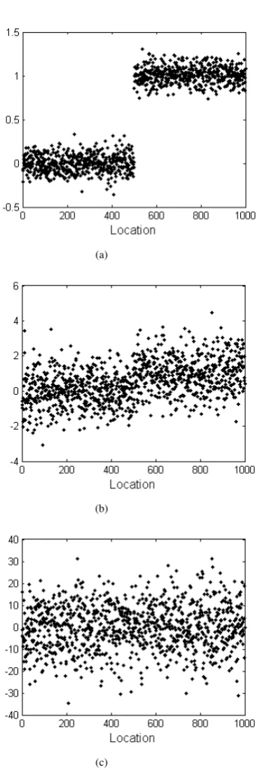
Weak mean difference data (WMDD) are representative of a type of data in which the information of the mean difference is reduced by a large variance. For example, as shown in Fig. (1), when the mean difference significantly exceeds the standard deviation, the location of the change point is easily detected. If the standard deviation is too large to cover the information of the mean difference, then the accuracy of change point detection may be decreased, and the location of the change point can hardly be detected by current models.
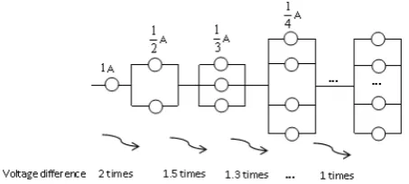
An important example of WMDD originated in the re-liability field. Assume that the resistance values of all the components in Fig. (2) are equal. Jin et al. [46] pointed out that components that are tested in a laboratory environment differ in significant ways from those that have experienced operations in fielded systems, as the fielded environment will cause homogeneous components to suffer different degrees of damage. As shown below, the voltages of components belonging to adjacent parallel structures become closer as the number of components belonging to the same level of parallel structure increases, which means that the lifetime difference in components belonging to adjacent parallel structures be-comes extremely small. To restore the system structure, we must differentiate the components that belong to different levels of parallel structures. As is known, components in the same level of parallel structures have homogeneous lifetime data. Hence, detecting the weak lifetime difference in components is extremely important to distinguish whether components belong to the same level of parallel structure and helps to establish a topology diagram of the system structure.
The difficulty of detecting change points for WMDD lies in capturing the small differences between subsignals. To solve this problem, we perform two enhanced operations to increase the mean difference between subsignals by utilizing the variance. In addition, we analyze the asymptotic proper-ties of the enhanced data. Next, we propose a strengthened change point detection model (SCPDM) according to the asymptotic results. Finally, we compare the SCPDM with two current models and verify that the SCPDM has a higher efficiency in terms of change point detection for WMDD by simulation analysis.
The paper is organized as follows. In II, the two enhanced operations and their asymptotic properties are provided. Based on asymptotic results, SCPDM is proposed. In Section III, using simulation analysis, we verify the correctness of theorem 2 and its remark. In addition, the SCPDM and the other two detection models are compared. The paper con-cludes with Section IV, which discusses the study findings and future implications.
(a)
(b)
[image:2.595.352.536.112.663.2](c)
Fig. 1. Diagram of the difficulty in change point detection that is influenced by various ratios between the variance and mean difference. The figures represent points from two normal distributions,N(µ1, σ2)andN(µ2, σ2).
(a)σ= 0.1,|µ1−µ2|= 1.(b)σ= 1,|µ1−µ2|= 1.(c)σ= 10,|µ1− µ2|= 1.
IAENG International Journal of Applied Mathematics, 50:1, IJAM_50_1_27
Fig. 2. Variation in the mean difference between components in the adjacent parallel structure. Because different components are subjected to different voltage intensities, the degree of deterioration over the lifetime varies by component; we can reflect the deterioration by the mean. When the resistance of the component is 1, then as the branch increases, the voltage experienced by the component is reduced.
II. METHODOLOGY
A. Two enhanced operations
Because the standard deviation is far larger than the mean difference, it is unwise and inefficient to perform change point detection for WMDD using traditional models. In fact, compared with the information of the mean difference, the variance is very remarkable and may supply more informa-tion. Therefore, we consider utilizing the variance that char-acterizes a type of disturbance information to analyze change points by performing the following two enhancements.
Now, we believe that t∗(t∗ ∈ {2,3, ..., T}) is the only abrupt location in sequence y1, ..., yT. For yt(t ∈
{2,3, ..., T}), we first conduct an operation called enhanced-I att and obtain the enhanced-I sequence y01, ..., y0T in (1).
y01=y1, y
0
i=min(yi−1, yi), i= 1, ..., t−1,
y0t=yt, y
0
i=max(yi−1, yi), i=t+ 1, ..., T. (1)
Then, we conduct a second operation, called enhanced-II at
t, and obtain the enhanced-II sequencey100, ..., yT00 in (2).
y100=y1, y
00
i =max(yi−1, yi), i= 1, ..., t−1,
yt00=yt, y
00
i =min(yi−1, yi), i=t+ 1, ..., T. (2)
Intuitively, these kinds of enhancements utilize the vari-ance information directly by taking a larger value or a smaller value between adjacent samples. Variance indicates the degree of fluctuation of the data, that is, in a set of data, the data is either larger or smaller according to the size of the variance centered on the mean. Therefore, when the first half of a set of data takes a smaller value (larger value) between adjacent samples, and the second half takes a larger value (smaller value), the mean difference of the strengthened data can well reflect the variance information.
To illustrate this, we generate normal random numbers with different means and variances. Then, under both en-hanced operations, the mean difference is calculated sepa-rately, as shown in Table. (I). It can be seen that the mean difference has nothing to do with the mean, and the mean difference is close to the variance.
Now, we provide several symbolic explanations. For a sig-nal sample y1, ..., yT, we perform the above two operations at location t(t∈ {2,3, ..., T}), where µ01(t, y
0
)indicates the sample mean of y10, ..., y0t−1; µ02(t, y0) indicates the sample mean of yt0, ..., y
0
T; µ
00
1(t, y
00
) indicates the sample mean of
y100, ..., y00t−1; and µ002(t, y00) indicates the sample mean of
yt00, ..., y00T. In addition, ◦ and • represent operations on the homogeneous signal sample and the signal sample containing a change point, respectively.
B. Asymptotic property of the enhanced sequence
We consider establishing a certain asymptotic property of the enhanced sequence in the following theorem. First, we point out that there are sufficient data for a signal sample. In other words, we assume that there are sufficient data before and after the location we are examining in a signal sample. When we consider yt, the assumption shows that there are sufficient data beforeyt. From the perspective of mathematics, it corresponds to t → ∞. Likewise, the exis-tence of sufficient data afteryt corresponds toT −t→ ∞. Furthermore, for a signal sample that has one change location att∗(t∗ ∈ {2, ..., T}), µ1 indicates the population mean of
the first subsignal, and µ2 indicates the population mean of
the second subsignal. σ2 indicates the constant population
variance. Generally, WMDD indicates that |µ2−µ1|
σ ≤1.
Theorem 1. Assume that y1, ..., yT are i.i.d., i.e., homo-geneous with a constant variance σ2. The above two
op-erations are performed nc times independently at location
t(t ∈ {2, ..., T}). Then, we have the following asymptotic property in (3).
P( lim
nc,t,T−t→∞
1 nc
nc
X
i=1
(|µ◦
0
1i(t, y
0
)
−µ◦
0
2i(t, y
0
)| − |µ◦
00
1i(t, y
00
)−µ◦
00
2i(t, y
00
)|) = 0) = 1 (3)
whereµ◦
0
1i(t, y
0
),µ◦
0
2i(t, y
0
),µ◦
00
1i(t, y
00
) and µ◦
00
2i(t, y
00
)|) rep-resent the mean in theith (i= 1,2, ..., nc) test sample.
Proof. Because y1, ..., yT are independent and identical-ly distributed, min(y1, y2), min(y2, y3),...,min(yT−1, yT) are identically distributed. We use µmin for the mean of min(yi, yj). Likewise, we use µmax for the mean of
max(yi, yj). Therefore, y
0
1, y
0
2, ..., y
0
t−1 are identically
dis-tributed according to the distribution of min(yi, yj),∀i 6=
j, i, j∈ {1,2, ..., T}. According to the law of large numbers, we have the following:
◦
µ
0
1i(t, y
0
)→µmin a.s. t→ ∞ (4)
Likewise, we have the following:
◦
µ
0
2i(t, y
0
)→µmax a.s. T−t→ ∞ (5)
As a result, we have the following in (6):
◦
µ
0
1i(t, y
0
)−µ◦
0
2i(t, y
0
)→µmin−µmax
a.s. t, T−t→ ∞ (6)
On the other hand, in (7):
◦
µ
00
1i(t, y
00
)→µmax a.s. t→ ∞
◦
µ
00
2i(t, y
00
)→µmin a.s. T−t→ ∞ (7)
Consequently, we have the following result in (8):
IAENG International Journal of Applied Mathematics, 50:1, IJAM_50_1_27
◦
µ
00
1i(t, y
00
)−µ◦
00
2i(t, y
00
)→µmax−µmin
a.s. t, T−t→ ∞ (8)
In addition, f(x, y) =|x| − |y| is a continuous function, and thus a.s. (almost sure) convergence can be preserved under the transformation of this function; therefore, we have the following (9):
|µ◦
0
1i(t, y
0
)−µ◦
0
2i(t, y
0
)| − |µ◦
00
1i(t, y
00
)−µ◦
00
2i(t, y
00
)|
→ |µmin−µmax| − |µmax−µmin|= 0
a.s. t, T−t→ ∞ (9)
Thus, because the process is independently performed nc
times,|µ◦
0
1i(t, y
0
)−µ◦
0
2i(t, y
0
)| − |µ◦
00
1i(t, y
00
)−µ◦
00
2i(t, y
00
)|(i= 1, ..., nc) can be viewed as independently and identically distributed. According to the law of large numbers, we have the following (10):
1 nc
nc
X
i=1
(|µ◦
0
1i(t, y
0
)−µ◦
0
1i(t, y
0
)| − |µ◦
00
1i(t, y
00
)−µ◦
00
1i(t, y
00
)|)
→0 a.s. t, T −t→ ∞, nc→ ∞ (10)
Remark 1. Theorem 1 demonstrates that, wheny1, ..., yT are homogeneous and the above two operations are per-formed nc times independently at any location t(t ∈
({2, ..., T})), the value of n1
c
nc
P i=1
|µ◦
00
1i(t, y
0
)−µ◦
00
2i(t, y
0
)| −
|µ◦
00
1i(t, y
00 −µ◦
00
2i(t, y
00
)|fluctuates at approximately 0. Next, we will give the asymptotic property when there is only one change point among the signal samples. We will present the asymptotic results about the position of the change point.
Theorem 2. Assume that the independent y1, ..., yT has only one change point t∗ with a constant variance σ2. At
t∗, the above two enhanced operations are independently performednctimes. Then, we have the following asymptotic property:
(1) if |µ1−µ2|
σ >1, then we have (11):
P( lim
nc,t∗,T−t∗→∞
1 nc
nc
X
i=1
(||µ•
0
1i(t∗, y
0
)
−µ•
0
2i(t ∗, y0
)| − |µ•
00
1i(t ∗, y00
)−µ•
00
2i(t ∗, y00
)||
−(|µ◦
0
1i(t∗, y
0
)−µ◦
0
2i(t∗, y
0
)|+|µ◦
00
1i(t∗, y
00
)−µ◦
00
2i(t∗, y
00
)|))
= 0) = 1 (11)
The meanings of µ◦
0
1i(t∗, y
0
),µ◦
0
2i(t∗, y
0
),µ◦
00
1i(t∗, y
00
) and ◦
µ
00
2i(t∗, y
00
)are the same as in theorem 2. (2) if |µ1−µ2|
σ ≤1, then we have (12):
P( lim
nc,t∗,T−t∗→∞
1 nc
nc
X
i=1
(||µ•
0
1i(t ∗, y0
)
−µ•
0
2i(t∗, y
0
)|−|µ•
00
1i(t∗, y
00
)−µ•
00
2i(t∗, y
00
)||) = 2|µ2−µ1|) = 1
(12)
Proof. (1) First, we prove the first part. The following formula is clear whenµ1< µ2, in (13)
|µ•
0
1i(t ∗, y0
)−µ•
0
2i(t ∗, y0
)| − |µ◦
0
1i(t ∗, y0
)−µ◦
0
2i(t ∗, y0
)| →(µ2−µ1)→a.s. t∗, T −t∗→ ∞ (13)
Because |µ1−µ2|
σ > 1, an incorrect enhanced operation cannot reverse the direction of the mean difference; therefore, we have the following (14):
|µ•
00
1i(t∗, y
00
)−µ•
00
2i(t∗, y
00
)|+|µ◦
00
1i(t∗, y
00
)−µ◦
00
2i(t∗, y
00
)|
→(µ2−µ1)→a.s. t∗, T −t∗→ ∞ (14)
Therefore,
|µ•
0
1i(t ∗, y0
)−µ•
0
2i(t ∗, y0
)| − |µ•
00
1i(t ∗, y00
)−µ•
00
2i(t ∗, y00
)|
−(|µ◦
0
1i(t∗, y
0
)−µ◦
0
2i(t∗, y
0
)|+|µ◦
00
1i(t∗, y
00
)−µ◦
00
2i(t∗, y
00
)|)
→0 a.s. t∗, T −t∗→ ∞ (15)
Likewise, when µ1 > µ2, we have the following two
relationships in (16) and (17):
|µ•
0
1i(t ∗, y0
)−µ•
0
2i(t ∗, y0
)|
+|µ◦
0
1i(t ∗, y0
)−µ◦
0
2i(t ∗, y0
)| →(µ1−µ2)→a.s. t∗, T −t∗→ ∞
(16)
|µ•
00
1i(t ∗, y00
)−µ•
00
2i(t ∗, y00
)|
− |µ◦
00
1i(t∗, y
00
)−µ◦
00
2i(t∗, y
00
)| →(µ1−µ2)→a.s. t∗, T −t∗→ ∞
(17)
Therefore,
|µ•
00
1i(t∗, y
00
)−µ•
00
2i(t∗, y
00
)| − |µ•
0
1i(t∗, y
0
)−µ•
0
2i(t∗, y
0
)|
−(|µ◦
0
1i(t ∗, y0
)−µ◦
0
2i(t ∗, y0
)|+|µ◦
00
1i(t ∗, y00
)−µ◦
00
2i(t ∗, y00
)|)
→0 a.s. t∗, T −t∗→ ∞ (18)
In summary, we have the following in (19):
||µ•
0
1i(t∗, y
0
)−µ•
0
2i(t∗, y
0
)| − |µ•
00
1i(t∗, y
00
)−µ•
00
2i(t∗, y
00
)||
−(|µ◦
0
1i(t ∗, y0
)−µ◦
0
2i(t ∗, y0
)|+|µ◦
00
1i(t ∗, y00
)−µ◦
00
2i(t ∗, y00
)|)
→0 a.s. t∗, T −t∗→ ∞ (19)
Thus, because the process is independently performed
nc times, || •
µ
0
1i(t∗, y
0
) − µ•
0
2i(t∗, y
0
)| − |µ•
00
1i(t∗, y
00
) −
•
µ
00
2i(t∗, y
00
)|| −(|µ◦
0
1i(t∗, y
0
)−µ◦
0
2i(t∗, y
0
)|+|µ◦
00
1i(t∗, y
00
)−
◦
µ
00
2i(t∗, y
00
)|)can be viewed as being independent and iden-tically distributed. According to the law of large numbers, we have the following in (20):
IAENG International Journal of Applied Mathematics, 50:1, IJAM_50_1_27
1 nc
nc
X
i=1
(||µ•
0
1i(t ∗, y0
)−µ•
0
2i(t ∗, y0
)|−|µ•
00
1i(t ∗, y00
)−µ•
00
2i(t ∗, y00
)||
−(|µ◦
0
1i(t∗, y
0
)−µ◦
0
2i(t∗, y
0
)|+|µ◦
00
1i(t∗, y
00
)−µ◦
00
2i(t∗, y
00
)|))→0
a.s. t∗, T −t∗, nc→ ∞ (20)
Proof. (2) The following formula in (21) is clear when
µ1< µ2,
|µ•
0
1i(t∗, y
0
)−µ•
0
2i(t∗, y
0
)| − |µ◦
0
1i(t∗, y
0
)−µ◦
0
2i(t∗, y
0
)|
→(µ2−µ1)→a.s. t∗, T −t∗→ ∞ (21)
Due to |µ2−µ1|
σ ≤1, the enhanced operation can reverse the mean difference, and thus we have the following in (22):
|µ•
00
1i(t∗, y
00
)−µ•
00
2i(t∗, y
00
)| − |µ◦
00
1i(t∗, y
00
)−µ◦
00
2i(t∗, y
00
)|
→ −(µ2−µ1)→a.s. t∗, T −t∗→ ∞ (22)
Likewise, when µ1 > µ2, we have the following two
relationships in (23)and (24):
|µ•
0
1i(t∗, y
0
)−µ•
0
2i(t∗, y
0
)| − |µ◦
0
1i(t∗, y
0
)−µ◦
0
2i(t∗, y
0
)| → −(µ1−µ2)→a.s. t∗, T −t∗→ ∞
(23)
|µ•
00
1i(t∗, y
00
)−µ•
00
2i(t∗, y
00
)| − |µ◦
00
1i(t∗, y
00
)−µ◦
00
2i(t∗, y
00
)|
→(µ1−µ2)→a.s. t∗, T −t∗→ ∞ (24)
Thus, in (25)
||µ•
0
1i(t ∗, y0
)−µ•
0
2i(t ∗, y0
)| − |µ•
00
1i(t ∗, y00
)−µ•
00
2i(t ∗, y00
)||
→2|µ2−µ1| a.s. t∗, T −t∗→ ∞ (25)
Because the process is independently performed nc times,
||µ•
0
1i(t∗, y
0
)−µ•
0
2i(t∗, y
0
)| − |µ•
00
1i(t∗, y
00
)−µ•
00
2i(t∗, y
00
)||(i= 1, ..., nc) can be viewed as being independently and identi-cally distributed. Therefore, we have the following in (26):
1 nc
nc
X
i=1
(||µ•
0
1i(t∗, y
0
)−µ•
0
1i(t∗, y
0
)|−|µ•
00
1i(t∗, y
00
)−µ•
00
1i(t∗, y
00
)||
→2|µ2−µ1| a.s. t, T−t, nc→ ∞ (26)
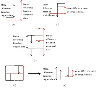
Remark 2. For (13), (14), (21) and (22), we provide the four schematic diagrams, as shown in Fig. (5). to illustrate the establishment of the four formulas. The black lines in the figure represent original data at different mean levels, whereas the red lines indicate enhanced data at different mean levels.
Remark 3.For WMDD, theorem 2 demonstrates that when
y1, ..., YT has a change at t∗(t∗ ∈2, ..., T)and if the above two operations are performed nc times independently at
t∗(t∗ ∈ 2, ..., T), then the value of n1
c
nc
P i=1
(||µ•
0
1i(t∗, y
0
)−
•
µ
0
1i(t∗, y
0
)| − |µ•
00
1i(t∗, y
00
)−µ•
00
1i(t∗, y
00
)||will reach the value
2|µ2−µ1|. Furthermore, by theorem 1, we know that at
any non-change location, n1
c
nc
P i=1
(||µ•
0
1i(t∗, y
0
)−µ•
0
1i(t∗, y
0
)| − |µ•
00
1i(t∗, y
00
)−µ•
00
1i(t∗, y
00
)||will becomen1
c
nc
P i=1
(||µ◦
0
1i(t∗, y
0
)−
◦
µ
0
1i(t∗, y
0
)| − |µ◦
00
1i(t∗, y
00
)−µ◦
00
1i(t∗, y
00
)||. Because the data exemplify the weak mean difference, this value will still approximate zero. Therefore, if the above two operations are performed nc times independently at any non-change
location, then the value ofn1
c
nc
P i=1
(||µ•
0
1i(t∗, y
0
)−µ•
0
1i(t∗, y
0
)|−
|µ•
00
1i(t∗, y
00
)−µ•
00
1i(t∗, y
00
)||will be less than the value2|µ2−
µ1|. The latter finding is verified in Section 3 in detail.
C. SCPDM
For WMDD, the different asymptotic properties in theorem 1 and theorem 2 are important information for judging whether there is a change point and the location of the change point. Consequently, we propose a model for detecting the change point in WMDD by sampling repeatedly in this section.
Assume that there is only one change point whose location ist∗(1< t∗≤T)iny1, ..., yT. To obtain a better estimate of
t∗, we should establish a contrast function [5] to measure the goodness-of-fit of the signal sample. First, att(t= 2, ..., T), the above two enhanced operations are performednc times. The following contrast function is established in (23):
ˆ
t∗(y) =argmax 1 nc
nc
X
i=1
(||µ•
0
1i(t∗, y
0
)
−µ•
0
2i(t∗, y
0
)| − |µ•
00
1i(t∗, y
00
)−µ•
00
1i(t∗, y
00
)|| (23)
According to theorem 2, the value of||
•
µ01
t
−
•
µ02
t
|−|
•
µ001
t
−
•
µ002
t
||
is expected to be large whent∗ is well-estimated.
During the establishment of the SCPDM, solving this discrete optimization problem becomes clear. We
need only to calculate n1
c
nc
P i=1
(||µ•
0
1i(t∗, y
0
)−µ•
0
2i(t∗, y
0
)| −
|µ•
00
1i(t∗, y
00
)−µ•
00
1i(t∗, y
00
)||at (t=2,...,T) and to makeˆt∗(y) =
argmax1
nc
nc
P i=1
(||µ•
0
1i(t∗, y
0
)−µ•
0
2i(t∗, y
0
)| − |µ•
00
1i(t∗, y
00
)−
•
µ
00
1i(t∗, y
00
)||. Details are elaborated in the next section, where we perform several simulation studies to estimatet∗under a normal distribution with various kinds of parameters.
III. VALIDATION OF THE METHODOLOGY
In this section, we will perform simulation analysis in two parts. In the first part, we verify the correctness of theorem 2 and remark 2. In the second part, we perform several simulation studies to estimate the potential location of change points under a normal distribution with different parameters and compare the SCPDM with two current models to verify that the SCPDM has a higher efficiency than those of the other models for WMDD.
A. Verifying the correctness of the theorem
To verify the correctness of theorem 2, we generate random numbers based on the normal distribution, and the parameter settings are shown in the caption of each figure.
IAENG International Journal of Applied Mathematics, 50:1, IJAM_50_1_27
Fig. 3. The illustration of formula (13), (14), (21) and (22). (a) illustrates formula (13); (b) illustrates formula (14); (c) illustrates formula (21); The process from (d) to (e) illustrates formula (22)
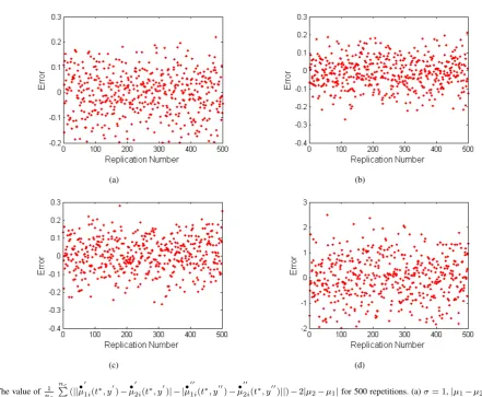
For the public parameters, we set T = 1000,t∗ = 501, and
nc = 1000. Both the number of data in the first half and the number in the second half are all 500, which can be considered large. Therefore, it can be seen as the case of
t∗→ ∞andT−t∗→ ∞. For |µ1−µ2|
σ >1, the asymptotic result should be near 0. We carry out two sets of simulation analyses. As shown in Fig. (4), simulated results agree with theoretical results.
When |µ1−µ2|
σ ≤ 1, as shown in Fig. (5), we carry out four sets of simulation analyses.
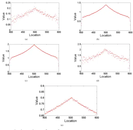
To verify the correctness of remark 2, when |µ1−µ2|
σ ≤1, at t(t = 400, ...,600), n1
c
nc
P i=1
(||µ•
0
1i(t∗, y
0
)−µ•
0
2i(t∗, y
0
)| −
|µ•
00
1i(t∗, y
00
)−µ•
00
2i(t∗, y
00
)||)is calculated, and the results are shown in Fig. (6).
It can be seen from Fig. (6) that whentis neart∗= 501,
1
nc
nc
P i=1
(||µ•
0
1i(t, y
0
)−µ•
0
2i(t, y
0
)| − |µ•
00
1i(t, y
00
)−µ•
00
2i(t, y
00
)||)
reaches a maximum value, which is approximately2|µ2−µ1|.
The simulation result is consistent with theorem 2.
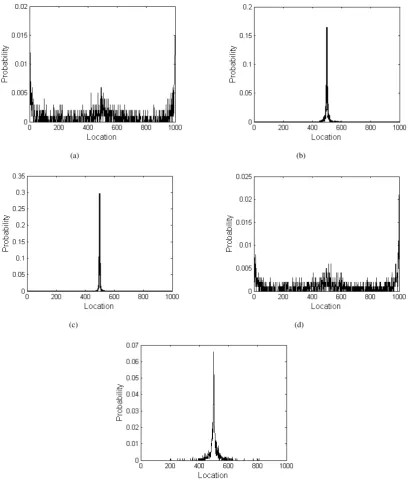
B. Model comparison
When |µ1−µ2|
σ ≤1, to verify that the SCPDM’s estimation of t∗ is better than that of the other models, we present certain simulation results based on traditional models, including the least squares model and Bayes method [47]. We generate random samplesy1, ..., yT based on the normal distribution, and the parameter settings are shown in the corresponding figure; we set the public parameters, namely,
T = 1000,t∗= 500, and nc = 1000. For the three models with the same parameter settings, we repeat the same
operation 1000 times, compute the estimation results of t∗ and regard the frequency of each ˆt∗ as the probability of being a real change point, which reflects the accuracy of each model. The results are shown in Fig. (7), Fig. (8) and Fig. (9).
When |µ1−µ2|
σ >1, i.e., the parameters are set to beσ=
0.5 and |µ1−µ2| = 1 for 1000 repeated tests, the least
squares model results inP r(ˆt∗ ∈ [499,503]) = 0.942 and
P r(ˆt∗ = 501) = 0.661, and the Bayes model results in
P r(ˆt∗∈[499,503]) = 0.87andP r(ˆt∗= 501) = 0.61. Both methods have a high accuracy for change point detection.
By setting different parameters, the detection accuracy of the change point interval, i.e., Pr(ˆt∗∈[499,503]), and change point location, i.e., Pr(ˆt∗ = 5.1), of the three models are compared in Table. (II), Table. (III), Table. (IV) and Table. (V).
When |µ1−µ2|
σ ≤1, the type of data is WMDD, and we considerP r(ˆt∗ ∈[499,503]). When the parameters are set toσ= 1and|µ1−µ2|= 0.1, the accuracy of the SCPDM
is 42%higher than that of the least squares model and 43%
higher than that of the Bayes model. When the parameters are set to σ = 1and |µ1−µ2| = 0.7, the accuracy of the
SCPDM is 54% higher than that of the least squares model and 60.7% higher than that of the Bayes model. When the parameters are set toσ= 1and|µ1−µ2|= 1, the accuracy
of the SCPDM is 31% higher than the accuracy of the least squares model and 41.1% higher than the accuracy of the Bayes model. When the parameters are set toσ = 10 and
|µ1−µ2|= 1, the accuracy of the SCPDM is 31%higher than
the accuracy of the least squares model and 41.1% higher than the accuracy of the Bayes model. When the parameters
IAENG International Journal of Applied Mathematics, 50:1, IJAM_50_1_27
(a) (b) The value of
Fig. 4. n1
c
nc
P i=1
(||µ• 0
1i(t∗, y
0
)−µ• 0
2i(t∗, y
0
)| − |µ• 00
1i(t∗, y
00
)−µ• 00
2i(t∗, y
00
)|| −(|µ◦ 0
1i(t∗, y
0
)−µ◦ 0
2i(t∗, y
0
)|+|µ◦ 00
1i(t∗, y
00
)−µ◦ 00
2i(t∗, y
00
)|))
for 500 repetitions. (a)σ= 0.1,|µ1−µ2|= 0.5. (b)σ= 1,|µ1−µ2|= 5.
(a) (b)
(c) (d)
The value of Fig. 5. n1
c
nc
P i=1
(||µ• 0
1i(t∗, y
0
)−•µ 0
2i(t∗, y
0
)| − |µ• 00
1i(t∗, y
00
)−µ• 00
2i(t∗, y
00
)||)−2|µ2−µ1|for 500 repetitions. (a)σ= 1,|µ1−µ2|= 0.1.
(b)σ= 1,|µ1−µ2|= 0.7. (c)σ= 1,|µ1−µ2|= 1. (d)σ= 10,|µ1−µ2|= 1.
IAENG International Journal of Applied Mathematics, 50:1, IJAM_50_1_27
[image:7.595.79.521.371.734.2](a) (b)
(c) (d)
[image:8.595.80.544.52.505.2](e) Fig. 6. The value ofn1
c
nc
P i=1
(||µ• 0
1i(t, y
0
)−µ• 0
2i(t, y
0
)|−|µ• 00
1i(t, y
00
)−•µ 00
2i(t, y
00
)||)at locationt. (a)σ= 1,|µ1−µ2|= 0.1. (b)σ= 1,|µ1−µ2|= 0.7.
(c)σ= 1,|µ1−µ2|= 1. (d)σ= 10,|µ1−µ2|= 1. (e)σ= 1,|µ1−µ2|= 0.4.
are set to σ = 1 and |µ1 −µ2| = 0.4, the accuracy of
the SCPDM is 62.6% higher than the accuracy of the least squares model and 70.1% higher than the accuracy of the Bayes model.
When |µ1−µ2|
σ ≤1, we consider P r(ˆt
∗ =t∗). When the parameters are set toσ= 1and|µ1−µ2|= 0.1, the accuracy
of the SCPDM is 9.1%higher than that of the least squares model and 9.5%higher than that of the Bayes model. When the parameters are set to σ = 1 and |µ1−µ2| = 0.7, the
accuracy of the SCPDM is 27.7% higher than that of the least squares model and 32.1%higher than that of the Bayes model. When the parameters are set to σ = 1 and |µ1−
µ2|= 1, the accuracy of the SCPDM is 25%higher than the
accuracy of the least squares model and 33.6% higher than the accuracy of the Bayes model. When the parameters are set toσ= 10and|µ1−µ2|= 1, the accuracy of the SCPDM
is 9.2% higher than the accuracy of the least squares model and 9.5%higher than the accuracy of the Bayes model. When the parameters are set to σ = 1 and |µ1−µ2| = 0.4, the
accuracy of the SCPDM is 23.2%higher than the accuracy of the least squares model and 28.8%higher than the accuracy of the Bayes model.
IV. CONCLUSIONS AND FUTURE STUDY
This paper focuses on detecting the change points for weak mean difference data. We perform asymptotic analysis and establish a strengthened change point detection model. According to theorem 2 (2), the enhanced sequence uses significant variance information so that the weak mean dif-ference increases from|µ1−µ2|to2|µ1−µ2|, which makes
the change point easier to detect and increases the accuracy of change point detection. In addition, for WMDD, the traditional methods can be improved by adding the sample capacity to the sequence. Meanwhile, for the same amount of data, the SCPDM greatly increases the efficiency of change point detection by repeatedly detecting sequences with the same data structure. Furthermore, repeated measurements are possible for the lifetime data of components at the
IAENG International Journal of Applied Mathematics, 50:1, IJAM_50_1_27
(a) (b)
(c) (d)
[image:9.595.109.520.58.550.2](e)
Fig. 7. Probability of each location becoming a change point in the least squares model.(a)σ= 1,|µ1−µ2|= 0.1.(b)σ= 1,|µ1−µ2|= 0.7.(c)σ=
1,|µ1−µ2|= 1.(d)σ= 10,|µ1−µ2|= 1.(e)σ= 1,|µ1−µ2|= 0.4.
same location. Hence, compared with traditional methods, the SCPDM can effectively detect change points. Although the accuracy of change point detection has been improved, this paper also has several limitations. First, we only discuss that y1, ..., yT are independent with a normal distribution and there exists only a single change point. Second, the reason why the relationship between|µ1−µ2|andσhas an
important influence on the accuracy of change point detection is not discussed in depth. We define the ratio boundary of WMDD based on only experience and simulations. In a future study, we will extend the SCPDM to other distribution types and multiple point detection. In addition, for theorem 2, we will reprove the theorem by introducing the relationship between|µ1−µ2|andσ.
REFERENCES
[1] D. Angelosante, G.B. Giannakis, Group lassoing change-points in piecewise-constant AR processes, EURASIP Journal on Advances in Signal Processing, 2012:70, 2012.
[2] E. S. Page, Continuous inspection schemes, Biometrika, vol. 41, no. 1/2, pp100–115, 1954.
[3] E. Page, A test for a change in a parameter occurring at an unknown point, Biometrika, vol. 42, no. 3/4, pp523–527, 1955.
[4] J. Bai, P. Perron, Computation and analysis of multiple structural change models, Journal of applied econometrics, vol. 18, no. 1, pp1–22, 2003. [5] C. Truong, L. Oudre, N. Vayatis, Selective review of offline change
point detection methods, arXiv preprint, arXiv:1801.00718, 2018. [6] H. Chernoff, S. Zacks, Estimating the current mean of a normal
distribution which is subjected to changes in time, The Annals of Mathematical Statistics, vol. 35, no. 3, pp999–1018, 1964.
[7] G. Lorden, Procedures for reacting to a change in distribution, The Annals of Mathematical Statistics, vol. 42, no. 6, pp1897–1908, 1971. [8] C. L. Mallows, Some comments on c p, Technometrics, vol. 15, no. 4,
pp661–675, 1973.
IAENG International Journal of Applied Mathematics, 50:1, IJAM_50_1_27
(a) (b)
(c) (d)
[image:10.595.239.355.688.754.2](e)
Fig. 8. Probability of each location becoming a change point in the Bayes model.(a)σ= 1,|µ1−µ2|= 0.1.(b)σ = 1,|µ1−µ2|= 0.7.(c)σ=
1,|µ1−µ2|= 1.(d)σ= 10,|µ1−µ2|= 1.(e)σ= 1,|µ1−µ2|= 0.4.
TABLE I
THE MEAN DIFFERENCE UNDER BOTH ENHANCED OPERATIONS FOR NORMAL RANDOM NUMBERS WITH DIFFERENT MEANS AND VARIANCES σ2= 0.1 σ2= 1
µ= 1 0.1025
0.1130
1.1244 1.0855
µ= 5 0.1170
0.1133
1.0722 1.1860
µ= 10 0.1084
0.1180
1.0814 1.1332
IAENG International Journal of Applied Mathematics, 50:1, IJAM_50_1_27
(a) (b)
(c) (d)
[image:11.595.130.466.694.751.2](e)
Fig. 9. Probability of each location becoming a change point in the SCPDM.(A)σ = 1,|µ1−µ2|= 0.1.(B)σ = 1,|µ1−µ2|= 0.7.(C)σ =
1,|µ1−µ2|= 1.(D)σ= 10,|µ1−µ2|= 1.(E)σ= 1,|µ1−µ2|= 0.4.
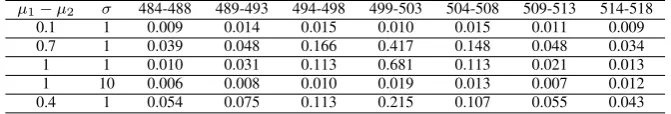
TABLE II
ESTIMATE OF THE PROBABILITY OF A CHANGE POINT IN CERTAIN INTERVALS FOR THE LEAST SQUARES METHOD µ1−µ2 σ 484-488 489-493 494-498 499-503 504-508 509-513 514-518
0.009 0.011
0.015 0.010
0.015 0.014
0.009 1
0.1
0.7 1 0.039 0.048 0.166 0.417 0.148 0.048 0.034 1 1 0.010 0.031 0.113 0.681 0.113 0.021 0.013 1 10 0.006 0.008 0.010 0.019 0.013 0.007 0.012 0.4 1 0.054 0.075 0.113 0.215 0.107 0.055 0.043
IAENG International Journal of Applied Mathematics, 50:1, IJAM_50_1_27
TABLE III
ESTIMATE OF THE PROBABILITY OF A CHANGE POINT IN CERTAIN INTERVALS FOR THEBAYES METHOD µ1−µ2 σ 484-488 489-493 494-498 499-503 504-508 509-513 514-518
0.1 1 0.01 0.03 0.01 0 0.02 0 0
0.7 1 0.06 0.06 0.18 0.35 0.18 0.07 0.01 1 1 0.01 0.02 0.11 0.58 0.13 0.07 0.03
1 10 0.01 0.01 0.01 0.01 0 0 0.01
0.4 1 0.02 0.04 0.08 0.14 0.10 0.06 0.02
TABLE IV
ESTIMATE OF THE PROBABILITY OF A CHANGE POINT IN CERTAIN INTERVALS FOR THESCPDMMETHOD µ1−µ2 σ 484-488 489-493 494-498 499-503 504-508 509-513 514-518
0.1 1 0.019 0.065 0.171 0.430 0.201 0.073 0.023
0.7 1 0 0 0.010 0.957 0.033 0 0
1 1 0 0 0.001 0.991 0.008 0 0
1 10 0.019 0.065 0.171 0.430 0.201 0.073 0.023
0.4 1 0 0 0.040 0.841 0.118 0.001 0
TABLE V
ESTIMATE OF THE PROBABILITY OFtˆ∗=t∗FOR THE THREE MODELS MD SD Least Squares Method Bayes Method SCPDM
0.1 1 0.004 0 0.095
0.7 1 0.164 0.12 0.441
1 1 0.286 0.2 0.536
1 10 0.003 0 0.095
0.4 1 0.066 0.01 0.298
[9] A. Sen, M. S. Srivastava, On tests for detecting change in mean, The Annals of Statistics, vol. 3, no. 1, pp98–108, 1975.
[10] V. Jandhyala, S. Fotopoulos, I. MacNeill, P. Liu, Inference for single and multiple change-points in time series, Journal of Time Series Analysis, vol. 34, no. 4, pp423–446, 2013.
[11] M. Lavielle, Detection of multiple changes in a sequence of dependent variables, Stochastic Processes and their Applications, vol. 83, no. 1, pp79 – 102, 1999.
[12] S. Chib, Estimation and comparison of multiple change-point mod-els, Journal of Econometrics, vol. 86, no. 2, pp221 – 241, 1998. http://dx.doi.org/https://doi.org/10.1016/S0304-4076(97)00115-2 [13] S. I. M. Ko, T. T. L. Chong, P. Ghosh, Dirichlet process hidden markov
multiple change-point model, Bayesian Analysis, vol. 10, no. 2, pp275– 296, 2015.
[14] J. Bai, Least squares estimation of a shift in linear processes, Journal of Time Series Analysis, vol. 15, no.5, pp.453–472, 1994.
[15] J. Bai, Least absolute deviation estimation of a shift, Econometric Theory, vol. 11, no. 3, pp403–436, 1995.
[16] J. Bai, Testing for parameter constancy in linear regressions: An empirical distribution function approach, Econometrica, vol. 64, no. 3, pp597–622, 1996.
[17] J. Bai, Vector Autoregressive Models with Structural Changes in Regression Coefficients and in Variance-Covariance Matrices, Annals of Economics and Finance, vol.1, no. 2, pp303-339.
[18] J. Bai, Estimation of a change point in multiple regression models, The Review of Economics and Statistics, vol. 79, no. 4, pp551–563, 1997.
[19] S. Arlot, A. Celisse, Z. Harchaoui, A kernel multiple change-point algorithm via model selection, arXiv preprint, arXiv:1202.3878, 2012. [20] F. Desobry, M. Davy, C. Doncarli, An online kernel change detection algorithm, IEEE Transactions on Signal Processing, vol. 53, no.8, pp2961–2974, 2005.
[21] Z. Harchaoui, O. Cappe, Retrospective mutiple change-point estima-tion with kernels, in: 2007 IEEE/SP 14th Workshop on Statistical Signal Processing, pp768–772, 2007.
[22] Z. Harchaoui, E. Moulines, F. R. Bach, Kernel change-point analysis, in: Advances in Neural Information Processing Systems 21, pp609–616, 2009.
[23] R. Lajugie, F. Bach, S. Arlot, Large-margin metric learning for con-strained partitioning problems, in: International Conference on Machine Learning, pp297–305, 2014.
[24] A. Gretton, K. M. Borgwardt, M. J. Rasch, B. Sch¨olkopf, A. J. Smola, A kernel method for the two-sample problem, CoRR, vol. abs/0805.2368, 2008.
[25] K. Jyrki, J. Alexander, C. W. Robert, Online learning with kernels, Signal Processing, IEEE Transactions, vol.52, no.8, pp2165-2176, 2004. [26] J. V. Davis, B. Kulis, P. Jain, S. Sra, I. S. Dhillon, Information-theoretic metric learning, in: Proceedings of the 24th International Conference on Machine Learning, ICML ’07, pp209–216, 2007.
[27] J. Friedman, T. Hastie, R. Tibshirani, The elements of statistical learning, vol.1, no.10, Springer series in statistics, New York, 2001. [28] E. P. Xing, M. I. Jordan, S. J. Russell, A. Y. Ng, Distance metric
learn-ing with application to clusterlearn-ing with side-information, in: Advances in neural information processing systems, pp. 521–528, 2003. [29] M. Csorgo, L. Horv´ath, Limit theorems in change-point analysis, John
Wiley & Sons, Chichester, 1997.
[30] Z. Kander, S. Zacks, Test procedures for possible changes in param-eters of statistical distributions occurring at unknown time points, The Annals of Mathematical Statistics, vol. 37, no.5, pp1196–1210, 1966. [31] L. A. Gardner, On detecting changes in the mean of normal variates,
The Annals of Mathematical Statistics, vol. 40, no. 1, pp116–126, 1969. [32] V. Jandhyala, C. Minogue, Distributions of bayes-type change-point statistics under polynomial regression, Journal of Statistical Planning and Inference, vol. 37, no. 3, pp271 – 290, 1993.
[33] V. K. Jandhyala, I. B. MacNeill, Iterated partial sum sequences of regression residuals and tests for changepoints with continuity con-straints, Journal of the Royal Statistical Society: Series B (Statistical Methodology), vol. 59, no. 1, pp147–156, 1997.
[34] S. B. Fotopoulos, V. K. Jandhyala, E. Khapalova, Exact asymptotic distribution of change-point mle for change in the mean of gaussian sequences, The Annals of Applied Statistics, vol. 4, no. 2, pp1081– 1104, 2010.
[35] S. B. Fotopoulos, V. K. Jandhyala, E. A. Khapalova, Change-point mle in the rate of exponential sequences with application to indonesian seismological data, Journal of Statistical Planning and Inference, vol. 141, no. 1, pp220 – 234, 2011.
[36] D. Hawkins, A. Gallant, W. Fuller, A simple least squares method for estimating a change in mean, Communications in Statistics-Simulation and Computation, vol. 15, no. 3, pp523–530, 1986.
[37] Y.-C. Yao, Approximating the distribution of the maximum likelihood estimate of the change-point in a sequence of independent random variables, The Annals of Statistics, vol. 15, no. 3, pp1321–1328, 1987. [38] A. Pettitt, A simple cumulative sum type statistic for the change-point problem with zero-one observations, Biometrika, vol. 67, no. 1, pp79– 84, 1980.
[39] E. Gombay, Comparison of u-statistics in the change-point problem and in sequential change detection, Periodica Mathematica Hungarica, vol. 41, no. 1, pp157–166, 2000.
IAENG International Journal of Applied Mathematics, 50:1, IJAM_50_1_27
[40] R. Killick, P. Fearnhead, I. A. Eckley, Optimal detection of change-points with a linear computational cost, Journal of the American Statistical Association, vol. 107, no. 500, 1590–1598, 2012.
[41] Z. L. Zabolotnii, Serhii W.and Warsza, Semi-parametric estimation of the change-point of parameters of non-gaussian sequences by polynomi-al maximization method, in: R. Szewczyk, C. Zieli´nski, M. Kpolynomi-aliczy´nska (Eds.), Challenges in Automation, Robotics and Measurement Tech-niques, Springer International Publishing, Cham, pp903–919, 2016. [42] E. C. Garcia, E. Gutierrez-Pe˜na, Nonparametric product partition
models for multiple changepoints analysis, Communications in Statistics -Simulation and Computation, vol. 48, no. 7, pp1922–1947, 2019. [43] R. Tibshirani, Regression shrinkage and selection via the lasso, Journal
of the Royal Statistical Society: Series B (Methodological), vol. 58, no. 1, pp267–288, 1996.
[44] R. Tibshirani, M. Saunders, S. Rosset, J. Zhu, K. Knight, Sparsity and smoothness via the fused lasso, Journal of the Royal Statistical Society: Series B (Statistical Methodology), vol. 67, no. 1, pp91–108, 2005. [45] R. Tibshirani, P. Wang, Spatial smoothing and hot spot detection for
CGH data using the fused lasso, Biostatistics, vol. 9, no.1, pp18–29, 2007.
[46] Y. Jin, P. G. Hall, J. Jiang, F. J. Samaniego, Estimating component reliability based on failure time data from a system of unknown design, Statistica Sinica, vol. 27, no. 2, pp479–499, 2017.
[47] C. Erdman, J. W. Emerson, et al., bcp: an r package for performing a bayesian analysis of change point problems, Journal of Statistical Software, vol. 23, no. 3, pp1–13, 2007.
Qi Zhouwas born in HeBei, China, in 1993. He received a bachelor’s degree in statistics from North China University of Science and Technology. His main research interests are statistics, linear Bayesian estimator, change point analysis and simulation.
Shaoqian Huang was born in HeBei, China, in 1994. He received a bachelor’s degree in statistics from North China University of Science and Technology. His main research interests are statistics, linear Bayesian estimator, change point analysis and simulation.