Advantages of VCG Auction based Relay Algorithm for DTNs

(1)

Advantages of VCG Auction based Relay Algorithm for

DTNs

Gulnaz Malled

JNTUA

CSE, Kuppam Engineering College, AP India

Logesh K.

JNTUA

CSE, Kuppam Engineering College, AP India

ABSTRACT

Wireless Mobile ad hoc networks use Delay/disruption tolerant technology in order to make up for the lack of end to end connectivity. DTNs work in store-carry-forward fashion to deliver messages with opportunistic encounters of nodes. And this strategy consumes resources such as storage and energy. This could well be the reason for nodes to avoid message forwarding, to save their limited resources. This kind of selfish behavior hinders communication. In order to stimulate participation of nodes for a smooth communication incentives are awarded. An efficient Incentive-Compatible-Routing Protocol (ICRP) with multiple copies for two-hop DTNs by using optimal sequential stopping rule and algorithmic game theory will be used. Relaying nodes can receive the maximum reward only when they honestly report the true encounter probability and routing metrics, which will stimulate nodes to participate in the relay node selection process. To implement this Vickrey-Clarke-Groves (VCG) Auction (second-price sealed-bid) based algorithm is employed as a strategy to refine the relay node selection process. ICRP attempts to find the optimal stopping time threshold adaptively based on realistic probability model and propose an algorithm to calculate the threshold. Based on this threshold, it proposes a new method to select relay nodes for multi-copy transmissions. ICRP can effectively stimulate nodes to carry/forward messages and achieve higher packet

delivery ratio with lower transmission cost. This

implementation reduces the end-to-end delay, energy consumption. And it ensures the existence of more number of live nodes.

General Terms

Node, Network, Routing information, Delay tolerant networks (DTNs)

Keywords

Epidemic Algorithm, Incentive Compatible routing algorithm (ICRP), optimal sequential stopping rule, VCG based auction Algorithm.

1. INTRODUCTION

In order to communicate between ad hoc wireless nodes a technology is used which is known as delay tolerant DTN [1]. Delay tolerance is needed because MANETs do not have either infrastructure or end to end connectivity between source and destination nodes to establish routes. Therefore nodes need to store-carry-forward the messages till they meet the destination node.

Of late, the term disruption-tolerant networking has taken root in the United States due to support from DARPA, which has funded many DTN projects. Disruption may occur because of the limits of wireless radio range, sparsely spread mobile nodes, energy resources, attack, and noise.

In efforts to provide a shared framework for algorithm and application development in DTNs, RFC 4838 and RFC 5050 were published in 2007 to define a common abstraction to software running on disrupted networks. Commonly known as the Bundle Protocol, this protocol defines a series of contiguous data blocks as a bundle—where each bundle contains enough semantic information to allow the application to make progress where an individual block may not. Bundles are routed in a store and forward manner between participating nodes over varied network transport technologies (including both IP and non-IP based transports). The transport layers carrying the bundles across their local networks are called bundle convergence layers. The bundle architecture therefore operates as an overlay network, providing a new naming architecture based on Endpoint Identifiers (EIDs) and coarse-grained class of service offerings.

Protocols using bundling must leverage application-level preferences for sending bundles across a network. Due to the store and forward nature of delay-tolerant protocols, routing solutions for delay-tolerant networks can benefit from exposure to application-layer information. For example, network scheduling can be influenced if application data must be received in its entirety, quickly, or without variation in packet delay. Bundle protocols collect application data into bundles that can be sent across heterogeneous network configurations with high-level service guarantees. The service guarantees are generally set by the application level, and the RFC 5050 Bundle Protocol specification includes "bulk", "normal", and "expedited" markings.

The ability to transport, or route, data from a source to a destination is a fundamental ability all communication networks must have. Delay and disruption-tolerant networks (DTNs), are characterized by their lack of connectivity, resulting in a lack of instantaneous end-to-end paths. In these challenging environments, popular ad hoc routing protocols

such as AODVand DSR fail to establish routes [2]. This is

(2)

opportunities are more tightly constrained, a more discriminate algorithm is required.

DTN is a suite of protocols as a result of research and development by members of Disruption Tolerant Networking Research Group as Requests for Comment (RFCs) administered by the Internet Engineering Task Force (IETF). This technology is best suited for interplanetary networking

2. RELATED WORKS

The initial research in DTNs focuses on how to design efficient message delivery schemes based on opportunistic transmissions. Most papers assume that there are no selfish nodes in the sense that each node forwards messages for others.

S. Burleigh et.al [3] describe that, increasingly, network applications must communicate with counterparts across

disparate networking environments characterized by

significantly different sets of physical and operational constraints; wide variations in transmission latency are particularly troublesome. The proposed Interplanetary Internet, which must encompass both terrestrial and interplanetary links, is an extreme case. An architecture based on a "least common denominator" protocol that can operate successfully and (where required) reliably in multiple disparate environments would simplify the development and deployment of such applications. The Internet protocols are ill suited for this purpose. The Authors identify three fundamental principles that would underlie a delay-tolerant networking (DTN) architecture and describe the main structural elements of that architecture, centered on a new end-to-end overlay network protocol called Bundling. The Authors also examine Internet infrastructure adaptations that might yield comparable performance but conclude that the simplicity of the DTN architecture promises easier deployment and extension.

A. Chaintreau et.al[4] describe that — Studying transfer opportunities between wireless devices carried by humans, the authors observe that the distribution of the inter-contact time, that is the time gap separating two contacts of the same pair of devices, exhibits a heavy tail such as one of a power law, over a large range of value. This observation is confirmed on six distinct experimental data sets. It is at odds with the exponential decay implied by most mobility models. In this the authors study how this new characteristic of human mobility impacts a class of previously proposed forwarding algorithms. A simplified model based on the renewal theory to study how the parameters of the distribution impact the delay performance of these algorithms.

Thrasyvoulos Spyropoulos et.al [5] describe that

intermittently connected mobile networks are wireless networks where most of the time there does not exist a complete path from the source to the destination. There are many real networks that follow this model, for example, wildlife tracking sensor networks, military networks, vehicular ad hoc networks (VANETs), etc. In this context, conventional routing schemes would fail, because they try to

establish complete end-to-end paths, before any data is sent.

To deal with such networks researchers have suggested using flooding-based routing schemes. While flooding-based schemes have a high probability of delivery, they waste a lot of energy and suffer from severe contention which can significantly degrade their performance. With this in mind, the Authors look into a number of routing schemes that use only one copy per message, and hence significantly reduce the resource requirements of flooding-based algorithms.

R.S.Mangrulkar et.al[6] describe that to formulate the delay-tolerant networking routing problem, where messages are to be moved end-to-end across a connectivity graph that is

time-varying but whose dynamics may be known in advance. The

problem has the added constraints of finite buffers at each

nodeand the general property that no contemporaneous

end-to-end path may ever exist. This situation limits the applicability of traditional routing approaches that tend to treat outages as failures and seek to find an existing end-to-end path. The Authors propose a framework for evaluating routing algorithms in such environments. The Authors then develop several algorithms and use simulations to compare their performance with respect to the amount of knowledge they require about network topology. The Authors find that, as expected, the algorithms using the least knowledge tend to perform poorly. The Authors also find that with limited additional knowledge, far less than complete global knowledge; efficient algorithms can be constructed for routing in such environments. To the best of our knowledge this is the first such investigation of routing issues in DTNs.

Zhenseng Zhang [7] the author describes that The

introduction of intelligent devices with short range wireless communication techniques has motivated the development of Mobile Ad hoc Networks (MANETs) during the last few years. Traditional end-to-end based routing algorithms designed for MANETs are not much robust in the challenged networks suffering from frequent disruption, sparse network density and limited device capability. Such challenged networks, also known as Intermittently Connected Networks (ICNs) adopt the Store-Carry-Forward (SCF) behavior arising from the mobility of mobile nodes for message relaying. In this article, the Authors consider the term ICNs as Delay/Disruption Tolerant Networks (DTNs) for the purpose of generalization, since DTNs have been envisioned for different applications with a large number of proposed routing algorithms. Motivated by the great interest from the research community, the Authors firstly review the existing unicasting issue of DTNs because of its extensive research stage.

Kevin Fall et.al [8] review the rationale behind the current design of the Delay/Disruption Tolerant Networking (DTN) Architecture and highlight some remaining open issues. Its evolution, from a focus on deep space to a broader class of heterogeneous networks that may suffer disruptions, affected design decisions spanning naming and addressing, message formats, data encoding methods, routing, congestion management and security. Having now achieved relative stability with the design, additional experience is required in long-running operational environments in order to fine tune our understanding of DTN concepts and the types of capabilities that are worth the investment in implementation complexity. The authors expect key management, handling of congestion, multicasting capability, and routing to remain active areas of research and development, and that DTN may continue to be an active research endeavor for at least the next few years.

(3)

the probability distribution of future contact times and choose a proper next hop in order to improve the end-to-end delivery probability. The algorithm is based on two observations: one is that nodes usually move around a set of well visited landmark points instead of moving randomly; the other is that node mobility behavior is semi-deterministic and could be predicted once there is sufficient mobility history information. Specifically, our approach employs a time homogeneous semi-markov process model that describes node mobility as transitions between landmarks. Landmark transition and sojourn time probability distributions are determined from nodes‘ mobility history.

Jon Crowcroft et.al [10] describe that Challenged networks arise primarily as a result of various forms of host and router mobility, but may also come into being as a result of disconnection due to power management or interference. Examples of such networks include Terrestrial Mobile Networks, Exotic Media Networks, Military Ad-Hoc Networks, and Sensor and Sensor/Actuator Networks. The DTN architecture seeks to address the communication needs of these challenged environments through a message based store-and-forward overlay network that leverages a set of convergence layers to adapt to a wide variety of underlying transports. In addition, the model also espouses novel approaches to application structuring and programming interface, fragmentation, reliability, and persistent state management. The Haggle architecture builds on the original DTN architecture by providing a data-centric architecture. Applications do not have to concern themselves with the mechanisms of transporting data to the right place, since that makes them infrastructure-dependent. By delegating to Haggle‘s architecture the task of propagating data, applications can automatically take advantage of any connection opportunities that arise, both local neighborhoods opportunities and connectivity with servers on the Internet when available. This is clearly infeasible in the existing TCP/IP architecture.

Anders Lindgren et.al. [11] describe that Delay Tolerant Networking (DTN) has attracted a lot of attention from the research community in recent years. Much work has been done regarding network architectures and algorithms for routing and forwarding in such networks. At the same time as many show enthusiasm for this exciting new research area there are also many skeptics, who question the usefulness of research in this area. In the past, we have seen other research areas become over-hyped and later die out as there was no killer app for them that made them useful in real scenarios.

Real deployments of DTN systems have so far mostly been limited to a few niche scenarios, where they have been done as proof-of-concept field tests in research projects. The authors embark upon a quest to find out what characterizes potential killer applications for DTNs. Are there applications and situations where DTNs provide services that could not be achieved otherwise, or have potential to do it in a better way than other technique.

Sotirios-Angelos Lenas et.al [12] describe that Data streaming over Delay-Tolerant Networks (DTN) is a challenging task considering jointly the specific characteristics of DTN environments, the demanding nature of streaming applications and their wide applicability. Presently, there are not any advanced mechanisms available to support this functionality and typical configurations fail to efficiently transfer data streams. In this paper, the Authors present our ongoing work in data streaming over DTNs and propose the Bundle Streaming Service (BSS) as a framework to improve the reception and storage of data streams. Our proposed framework exploits the characteristics of Delay Tolerant Networks to allow for reliable delay-tolerant streaming. Here, the Authors present a simple usage scenario along with the proposed framework and evaluate it experimentally at a preliminary stage which suffices to demonstrate its potential suitability for both terrestrial and Space environments.

3. ALGORITHMS

The following section discusses all the various algorithms used for entire approach; the simulation is done using MATLAB.

3.1 Epidemic Routing Algorithm

Epidemic Routing algorithm is divided into multiple stages namely determine initiators, multiple route discovery, individual route discovery and finally best route discovery.

The process of initiator is used to find set of nodes within the transmission range. Each of the nodes will act as the first hop node towards destination.

Multiple route discoveries is responsible for finding routes by using one hop initiator towards destination by calling individual route discovery.

Individual route discovery is a process which has source node,

destination node and transmissionrange as input and then the

algorithm finds the individual route from source node to destination node. Best route selection is responsible for selecting the best route which has maximum trust level.

Obtain 1-hop neighbors

Obtain the count

i = 1

Perform ith route discovery Measure Delay

Store delay and route

i=i+1

(4)

Fig 1: Multiple Route Discovery

[image:4.595.61.273.141.495.2]

Fig 1 shows after obtaining 1 hop neighbors, measure the count starting from first node perform the route discovery and measure the end to end delay. Store key as delay and value as the route in hash map. This process is repeated until all the routes are found.

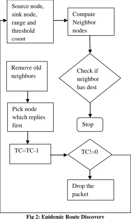
Fig 2: Epidemic Route Discovery

Individual Route Discovery

Individual route discovery is responsible for finding the single path between given source node and destination node. Source node, destination node, transmission range, threshold count are inputs to this algorithm. Compute the neighbor nodes if the neighbor nodes have destination then stop the routing process otherwise compute the REPLY TIME. The threshold count is decremented. This process is repeated until Threshold Count(TC) becomes zero or until destination is reached. Fig 2 depicts the full process based on epidemic route discovery.

Best Route Discovery

Epidemic Trust is defined as

𝐸𝑝𝑖𝑑𝑒𝑚𝑖𝑐 𝑡𝑟𝑢𝑠𝑡 =

𝐴𝑣𝑒𝑟𝑎𝑔𝑒 𝐷𝑒𝑙𝑎𝑦

𝑒𝑛𝑑 𝑡𝑜 𝑒𝑛𝑑 𝑑𝑒𝑙𝑎𝑦

∗ 𝑁 𝑝𝑎𝑐𝑘𝑒𝑡𝑠

The trust value is computed for all the routes. Pick the best route which has maximum trust.

3.2 Two Hop Relay Node based Routing

Two hop relay based route discovery is responsible for finding the end to end route by selection a relay node and when the relay node meets the destination at that time the packets are delivered to destination.

The relay node selection process can be described as follows

1) Number of iterations, Source Node and destination Node. 2) For each of the iteration perform the following

a) Find the neighbor of the Source Node

b) Find whether the neighbor can reach destination if Yes then 1 otherwise 0.

c) Store the neighbors in the traversed list. d) Generate a Non Traversed list

The virtual currency computation is performed using the following steps.

1) Source Node will send packets to neighbors. 2) Obtain the ACK count.

3) Find the value of the virtual currency=NACK/NSent. 4) If in a given iteration this process has happened then same node cannot be tested for next iteration.

After all iterations are completed compute the meeting probability and also get the cutoff threshold R. Each of the neighbor nodes count the number of times it meets every other node in the network for M rounds at the time instance {t1, t2, t3,...tm}

Each of the neighbors computes the probability.

𝑝𝑟𝑜𝑏𝑎𝑏𝑖𝑙𝑖𝑡𝑦 =𝑁𝑢𝑚𝑏𝑒𝑟 𝑜𝑓 𝑡𝑖𝑚𝑒𝑠 𝑎 𝑛𝑜𝑑𝑒 𝑖 𝑚𝑒𝑒𝑡𝑠 𝑚

Probability for Trust Level Distribution

The final probability is computed using the following equation

𝑃 = 𝑘 ×

1 𝑛

×

∁

_{𝑖−𝑟−1}𝑘−1

∁

_𝑛−1𝑘−1

×

𝑟

𝑖 − 𝑘

𝑖−𝑛

𝑖=𝑟+𝑘

Where,

k=Number of iterations

n=number of nodes

C=combination formula

r=threshold number (a point at which all nodes have met destination)

4. DATA ENCRYPTION PROCESS

Each data packet is transmitted securely using a digital signature and RSA algorithm is used for encryption at the source node and decryption at the destination node.

5. COMPARISON PARAMETERS

This section describes the various parameters which are used for comparison.

End to End Delay

End to End Delay is the time taken for the RREQ to go from the source node to destination node and then send back the RRPLY from destination node to source node.

E2Edelay= tstop - tstart

Where, tstop = It is the time at which RRPLY is received.

tstart = It is the time at which RREQ is sent

Source node,

sink node,

range and

threshold

count

Compute

Neighbor

nodes

Check if

neighbor

has dest

Remove old

neighbors

Stop

Pick node

which replies

first

Drop the

packet

(5)

Number of Hops

It is defined as the number of intermediate links between source node to destination node in the route.

Energy Consumed

The total energy consumption is given as follows

The energy consumed by the ith link given by

Energyconsumption = 2Etx + Egendδ

𝐸𝑡𝑥 = Energy required for transmission of control packet

Egen = energy required for packet generation

d= distance between nodes

δ= attenuation factor 0.1 ≤δ≤ 1

Egen << Etx

Battery Updating Process

Whenever a node participates in routing, then battery energy gets updated using the following equation.

Updated energy = | Current Energy – Energy Consumed|

if updated energy < 0

Updated energy = 0

Current Energy is the energy of node at current instant of time and energy consumed is the amount of energy consumed while sending the packets.

Number of Live Nodes

It is defined as the count of set of nodes whose battery level is greater than or equal to B/4 Where B is initial Battery power.

Number of Dead Nodes

It is defined as the count of set of nodes whose battery level is less than or equal to B/4 Where B is initial Battery power.

Routing Overhead

The routing overhead is defined as

𝑅𝑜𝑢𝑡𝑖𝑛𝑔 𝑂𝑣𝑒𝑟𝑕𝑒𝑎𝑑 =𝑁𝑢𝑚𝑏𝑒𝑟 𝑜𝑓 𝑐𝑜𝑛𝑡𝑟𝑜𝑙 𝑝𝑎𝑐𝑘𝑒𝑡𝑠 𝑁𝑢𝑚𝑏𝑒𝑟 𝑜𝑓 𝐷𝑎𝑡𝑎 𝑝𝑎𝑐𝑘𝑒𝑡𝑠

Lifetime Ratio

Lifetime ratio is defined as below

𝐿𝑖𝑓𝑒𝑡𝑖𝑚𝑒 =𝑁𝑢𝑚𝑏𝑒𝑟 𝑜𝑓 𝐴𝑙𝑖𝑣𝑒 𝑁𝑜𝑑𝑒𝑠 𝑁𝑢𝑚𝑏𝑒𝑟 𝑜𝑓 𝐷𝑒𝑎𝑑 𝑁𝑜𝑑𝑒𝑠

6. SIMULATION RESULTS

This section shows all the results related to Epidemic Algorithm.

Proposed method and comparison between them follows.

Epidemic Algorithm Input

Parameter Name Parameter Value

Number of Nodes 100

Transmission Range 40m

Energy Amplification 10mJ

Energy Transmission 20mJ

Attenuation Factor 0.7

Initial Battery Energy 4000mJ

Time to Live 8

Source Node 30

[image:5.595.310.545.71.262.2]

Destination Node 98

Fig 3: Battery Initialization

[image:5.595.334.522.316.492.2]

Fig 3 shows the initial battery power for the entire network. All the 100 nodes have been initialized with 4000mJ.

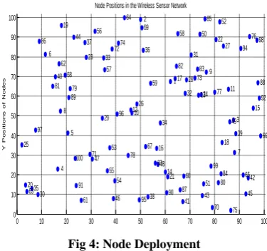
Fig 4: Node Deployment

[image:5.595.338.520.533.663.2]

Fig 4 shows node deployment of 100 nodes in 100*100m area.

[image:5.595.49.284.653.759.2]

Fig 5: Initial Trust level

Fig 5 shows the output of Trust Level algorithm. As shown in the figure there are 100 nodes and there trust level has a value of 1.

0 20 40 60 80 100 120

0 500 1000 1500 2000 2500 3000 3500 4000

Node Ids

B

a

tt

e

ry

P

o

w

e

r

in

m

J

Node Ids v/s Battery Power in mJ w.r.t WSN Network

0 10 20 30 40 50 60 70 80 90 100

X Positions of Nodes

Y

P

o

s

it

io

n

s

o

f

N

o

d

e

s

Node Positions in the Wireless Sensor Network

1 2

3

4 5 6

7 8

9

10

11 12

13

14

15

16 17

18 19

20

21

22 23

24

25

26

27

28

29

30

31

32 33

34

35

36 37

38

39 40

41

42 43 44

45 46

47

48

49 50

51 52

53

54 55 56

57

58

59

60

61 62

63

64

65 66 67

68

69

70 71

72

73 74

75 76

77

78 79

80 81

82 ₈₃

84 85

86

87

88 89

90 91

92

93

94

95 96 97

98

99 100

0 20 40 60 80 100 120

0 0.1 0.2 0.3 0.4 0.5 0.6 0.7 0.8 0.9 1

Node Ids

T

ru

s

t

L

e

v

e

ls

(6)

Fig 6: Initiators for node 30

Fig 6 shows all the neighbors for node 30 spread across 40m

Fig 7: RREQ/RRPLY for Route1

Fig 7 shows the RREQ/RRPLY process for the entire route. Blue color shows RREQ send to the neighbors and then red represents the RPLY packets.

Fig 8: Complete route for Route No. 1

Fig 8 shows the complete route 1 from source node 52 to destination node 73 with intermediate nodes 15,61,95,78 and 94 forms the complete route. Like this many routes are discovered and in this case it is 16 routes.

Fig 9: Trust Level Computation for Routes

Fig 9 shows the trust level computation for all the possible 16

routes. Among them route No.16th_{route is has the highest}

trust level. Hence it acts the best route.

Fig 9: Best Route Discovered in Epidemic algorithm

Fig 10 shows the best route discovered between source node 30 and destination node 98. Route No.16 is the best route with

intermediate nodes 100, 96 and 83.

Fig 11: Best Trust Level

Fig 11 shows the best route trust level is having a value of 425 as the overall best route calculated based on epidemic trust equation

0 5 10 15 20 25 30 35 40

0 5 10 15 20 25 30 35 40 45

Y P o s it io n s o f N o d e s

Initiator Nodes for Node = 30

4 5 20 25 35 46 47 53 54 55 61 63 71 91 97 100

0 10 20 30 40 50 60 70 80 90 100

RREQ/RRPLY for Route No = 1from Source Node to Destination Node

1 2 3 4 5 6 7 8 9 10 11 12 13 14 15 16 17 18 19 20 21 22 23 24 25 26 27 28 29 30 31 32 33 34 35 36 37 38 39 40 41 42 43 44 45 46 47 48 49 50 51 52 53 54 55 56 57 58 59 60 61 62 63 64 65 66 67 68 69 70 71 72 73 74 75 76 77 78 79 80 81

82 ₈₃

84 85 86 87 88 89 90 91 92 93 94 95 96 97 98 99 100

0 10 20 30 40 50 60 70 80 90 100

Route No = 1from Source Node to Destination Node

1 2 3 4 5 6 7 8 9 10 11 12 13 14 15 16 17 18 19 20 21 22 23 24 25 26 27 28 29 30 31 32 33 34 35 36 37 38 39 40 41 42 43 44 45 46 47 48 49 50 51 52 53 54 55 56 57 58 59 60 61 62 63 64 65 66 67 68 69 70 71 72 73 74 75 76 77 78 79 80 81

82 ₈₃

84 85 86 87 88 89 90 91 92 93 94 95 96 97 98 99 100

0 2 4 6 8 10 12 14 16 18

0 100 200 300 400 500 600 700 800 900 1000 Route No T r u s t L e v e l R o u t e

Route No v/s Trust Level Route

0 10 20 30 40 50 60 70 80 90 100 0 10 20 30 40 50 60 70 80 90 100

X positions of Nodes

Y p o s it io n s o f N o d e s

Best Route Discovered using Epedemic Route Discovery

1 2 3 4 5 6 7 8 9 10 11 12 13 14 15 16 17 18 19 20 21 22 23 24 25 26 27 28 29 30 31 32 33 34 35 36 37 38 39 40 41 42 43 44 45 46 47 48 49 50 51 52 53 54 55 56 57 58 59 60 61 62 63 64 65 66 67 68 69 70 71 72 73 74 75 76 77 78 79 80 81

82 ₈₃

84 85 86 87 88 89 90 91 92 93 94 95 96 97 98 99 100 16 0 100 200 300 400 500 600 700 800 900 1000

Best Route No

B e s t T r u s t L e v e l

(7)

[image:7.595.63.271.72.243.2]

Fig 12:Updated battery levels for Nodes

Fig 12 shows the updated battery level for all the nodes which participated in the all the possible 16 routes and depends on transmission energy, generation energy, attenuation factor and distance between the nodes.

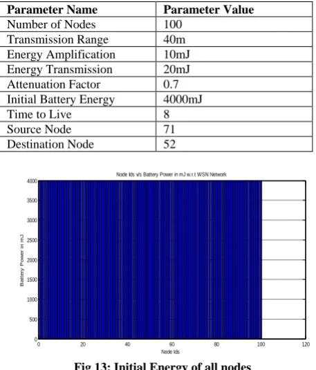
[image:7.595.317.534.79.256.2]

Two Hop Relay Algorithm Inputs

Fig 13: Initial Energy of all nodes

Fig 13 shows the initial battery power for all the 100 nodes in the network. All the nodes have been initialization with

4000mJ.

[image:7.595.332.538.283.451.2]

Fig14 shows node deployment of 100 nodes in 100*100m area.

Fig 15: Node Meeting Times

[image:7.595.49.278.324.592.2]

Fig 15 shows the node meeting times for all the 100 nodes in the network each bar indicates destination meets the node with what probability

Fig 16: Virtual Currency for Nodes

Fig 16 shows the virtual currency for all 100 nodes. It depends on the test packet delivery ratio.

0 20 40 60 80 100 120

0 500 1000 1500 2000 2500 3000 3500 4000

Node Ids in the Network

R

e

s

id

u

a

l

B

a

t

e

r

y

E

n

e

r

g

y

o

f

N

o

d

e

s

Node Ids in the Network v/s Residual Battery Energy of Nodes

0 20 40 60 80 100 120

0 500 1000 1500 2000 2500 3000 3500 4000

Node Ids

B

a

tt

e

ry

P

o

w

e

r

in

m

J

0 10 20 30 40 50 60 70 80 90 100

Y

P

o

s

it

io

n

s

o

f

N

o

d

e

s

1

2

3

4 5

6

7

8 9

10 11

12 13

14 15

16

17 18 19

20

21

22 23

24

25

26

27 28

29 30

31

32

33 34

35

36 37

38

39 40

41 42

43 44 45

46 47

48 49

50 51

52 53

54

55 56

57

58 59 60

61 62

63 64

65 66

67

68 69 70

71

72 73

74

75

76

77

78 79

80 81

82 83

84 85

86

87

88

89

90

91 92

93

94 95

96

97 98

99

100

0 20 40 60 80 100 120

0 10 20 30 40 50 60 70 80 90 100

Node Ids

M

e

ti

n

g

T

im

e

s

Nodes v/s Meeting Times

0 20 40 60 80 100 120

0 10 20 30 40 50 60 70 80 90 100

Node Ids

V

ir

tu

a

l

C

u

rr

e

n

c

y

Nodes v/s Virtual Currency

Parameter Name Parameter Value

Number of Nodes 100

Time to Live 8

Source Node 71

[image:7.595.324.526.496.645.2]

(8)

Fig 17: Trust Measure for nodes

Fig 17 shows the Trust measure of 100 nodes in the network. It depends on the probability, meeting probability and trust levels of nodes.

Fig 18: Relay Node Criteria

Fig 18 showsthe relay node criteria for all the 14 nodes in the

network. The node with highest criteria is 4016.63 and relay node 10.

Fig 19: 1st Communication Hop

Fig 19 shows 1st communication hop between node 10 and

node 71 for iteration number 1.

Fig 20: 2nd Communication hop

Fig 20 shows changes in positions of all nodes. In this iteration there is no communication because the destination is not in range of relay node.

Fig 21: Destination Communication hop

Fig 21 shows the communication between the relay node and destination node in the network.

Fig 22: Updated energy levels for nodes

Fig 22 shows the updated energy level of the nodes in the network. As shown in the figure node 10 and node 71 have lost their energy as they participated in routing.

0 20 40 60 80 100 120

0 500 1000 1500 2000 2500 3000 3500 4000 Node Ids T r u s t M e a s u r e N o d e W is e

Node Ids v/s Trust Measure Node Wise

0 5 10 15 20 25 30

0 500 1000 1500 2000 2500 3000 3500 4000 4500

Number of Neigbors

R e la y N o d e C ri te ri a

Nodes v/s Relay Node Criteria

0 10 20 30 40 50 60 70 80 90 100

X Position for the Nodes in the Network

Y P o s it io n f o r t h e N o d e s in t h e N e t w o r k

Positions for Nodes for Iteration =1

1 2 3 4 5 6 7 8 9 10 11 12 13 14 15 16 17 18 19 20 21 22 23 24 25 26 27 28 29 30 31 32 33 34 35 36 37 38 39 40 41 42 43 44 45 46 47 48 49 50 51 52 53 54 55 56 57 58 59 60 61

62 63

64 65 66 67 68 69 70 71 72 73 74 75 76 77 78 79 80 81 82 83 84 85 86 87 88 89 90 91 92 93 94 95 96 97 98 99 100

0 10 20 30 40 50 60 70 80 90 100 0 10 20 30 40 50 60 70 80 90 100

1 2 3 4 5 6 7 8 9 10 11 12 13 14 15 16 17 18 19 20 21 22 23 24 25 26 27 28 29 30 31 32 33 34 35 36 37 38 39 40 41 42 43 44 45 46 47 48 49 50 51

52 53

54 55 56 57 58 59 60 61

62 63

64 65 66 67 68 69 70 71 72 73 74 75 76 77 78 79 80 81 82 83 84 85 86 87 88 89 90 91 92 93 94 95 96 97 98 99 100

0 10 20 30 40 50 60 70 80 90 100

1 2 3 4 5 6 7 8 9 10 11 12 13 14 15 16 17 18 19 20 21 22 23 24 25 26 27 28 29 30 31 32 33 34 35 36 37 38 39 40 41 42 43 44 45 46 47 48 49 50 51 52 53 54 55 56 57 58 59 60 61

62 63

64 65 66 67 68 69 70 71 72 73 74 75 76 77 78 79 80 81 82 83 84 85 86 87 88 89 90 91 92 93 94 95 96 97 98 99 100

0 20 40 60 80 100 120

0 500 1000 1500 2000 2500 3000 3500 4000

(9)

[image:9.595.68.269.75.262.2]

Fig 23: Initial energy for all nodes

Fig 23 shows the initial battery power for all 100 nodes in the network. All the nodes have been initialized with 4000mJ

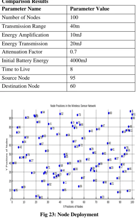
[image:9.595.323.533.76.258.2]

Comparison Results

As shown in the figure 100 nodes have been deployed in 100*100m area randomly.

Fig 24: End to End Delay

[image:9.595.51.280.302.664.2]

Fig 24 shows End to End Delay comparison between Two Hop Relay and Epidemic algorithm. As shown in figure Two Hop Relay has low End to End Delay as compared to epidemic algorithm.

Fig 25: Energy Consumption Comparison

[image:9.595.324.531.335.463.2]

Fig 25 shows the energy consumption comparison between Two Hop Relay Algorithm and Epidemic Algorithm. As shown in the figure Two Hop Relay algorithm has low energy consumption as compared to epidemic algorithm.

Fig 26: Number of Hops of Comparison

Fig 26 shows the number of hops comparison between two Hop Relay and Epidemic algorithm. As shown in figure two hops Relay algorithm has number hops as always 2 which is very less compared to epidemic algorithm.

0 20 40 60 80 100 120

0 500 1000 1500 2000 2500 3000 3500 4000

Node Ids

B

a

t

e

r

y

P

o

w

e

r

in

m

J

0 10 20 30 40 50 60 70 80 90 100

0 10 20 30 40 50 60 70 80 90

Y

P

o

s

it

io

n

s

o

f

N

o

d

e

s

1

2 3 4

5

6

7

8 9

10

11 12

13 14

15 16

17 18

19

20

21 22

23 24

25

26 27

28

29

30

31 32

33 34

35

36

37 38

39 40

41 42

43

44 45

46

47 48

49

50 51

52 53

54

55

56

57 58 59

60

61

62

63 64

65 66

67

68

69 70

71

72 73

74 75

76

77

78 79

80

81 82

83

84

85

86

87

88

89 90

91

92 93 94

95 96

97

98 99 100

0 5 10 15 20 25

0 0.1 0.2 0.3 0.4 0.5 0.6 0.7

Number of Routes

E

n

d

t

o

E

n

d

D

e

la

y

[

m

s

]

Performance - End to End Delay

EPEDIMIC TWO HOP RELAY

0 5 10 15 20 25

0 0.5 1 1.5 2 2.5 3 3.5 4 4.5x 10

4

Number of Routes

R

o

u

te

E

n

e

rg

y

C

o

n

s

u

m

p

ti

o

n

[

m

J

]

Comparision plot Route Energy Consumption

0 5 10 15 20 25

0 50 100 150 200 250 300 350

Number of Routes

N

u

m

b

e

r

o

f

H

o

p

s

Comparision plot Number of Hops

EPEDIMIC TWO HOP RELAY Parameter Name Parameter Value

Number of Nodes 100

Time to Live 8

Source Node 95

[image:9.595.324.530.532.695.2]

(10)

Fig 27: Number of live nodes

Fig 27 shows number of live nodes comparison between Two Hop relay algorithm and Epidemic algorithm. As shown in the figure two hop relay algorithm network has more number of live nodes.

Fig 28: Number of dead nodes

Fig 28 shows number of dead nodes comparison between Two Hop relay algorithm and Epidemic algorithm. As shown in the figure two hop relay algorithm network has less number of dead nodes.

Fig 29: Lifetime ratio

Fig 29 shows lifetime ratio comparison between Two Hop relay algorithm and Epidemic algorithm. As shown in the figure two hop relay algorithm network has more Lifetime as compared to Epidemic algorithm.

Fig 30: Residual Energy

Fig 30 shows Residual Energy comparison between Two Hop relay algorithm and Epidemic algorithm. As shown in the figure two hop relay algorithm network has more residual energy compared to epidemic algorithm.

Fig 31: Routing Overhead

Fig 31 shows routing overhead comparison between Two Hop relay algorithm and Epidemic algorithm. As shown in the figure two hop relay algorithm network has low routing overhead as compared to Epidemic algorithm

Fig 32: Energy Balancing Factor

Fig 32 shows Energy Balancing Factor comparison between Two Hop relay algorithm and Epidemic algorithm. As shown in the figure two hop relay algorithm network has a balanced level as compared to epidemic algorithm.

7. CONCLUSION

In this work the algorithm namely Epidemic algorithm and VCG Auction based Two Hop Relay algorithm which makes use of only 2-hops have been compared. Both the algorithms are compared on the parameters ‗End to End Delay‘, ‗Number of hops‘ ,‘ Total energy consumption‘, ‗number of Alive

0 5 10 15 20 25

0 10 20 30 40 50 60 70 80 90 100

Number of Routes

N

u

m

b

e

r

o

f

A

li

v

e

N

o

d

e

s

Comparision plot Number of Alive Nodes

0 5 10 15 20 25

0 10 20 30 40 50 60 70 80 90

Number of Routes

N

u

m

b

e

r

o

f

D

e

a

d

N

o

d

e

s

Comparision plot Number of Dead Nodes

0 5 10 15 20 25

0 10 20 30 40 50 60 70 80 90 100

Number of Routes

L

if

e

ti

m

e

R

a

ti

o

Comparision - Lifetime Ratio

0 5 10 15 20 25

0 0.5 1 1.5 2 2.5 3 3.5 4x 10

5

Number of Routes

R

e

s

id

u

a

l

E

n

e

rg

y

Comparision - Residual Energy

0 5 10 15 20 25

0 0.1 0.2 0.3 0.4 0.5 0.6 0.7

Number of Routes

R

o

u

t

in

g

O

v

e

r

h

e

a

d

Comparision - Routing Overhead

0 5 10 15 20 25

0 1 2 3 4 5 6 7 8 9 10

Number of Routes

E

n

e

rg

y

B

a

la

n

c

in

g

F

a

c

to

r

Comparision plot Number of Energy Balancing Factor

(11)

nodes‘,‘ number of Dead nodes‘,‘ Lifetime ratio‘, ‗Routing overhead‘ and ‗Energy balancing factor‘. The ICRP based two Hop algorithm outperforms Epidemic algorithm with respect all the parameters.

VCG auction and incentive based algorithm seems to be successful in dealing with selfish behavior of nodes in MANETS to a large extent and has higher delivery ratio and lower end to end delay.

It is possible that nodes may do false reporting to get forwarding opportunity. Or there may be nodes sending fake acknowledgement to get rewards. Although digital signature is used for secure transaction, there is a scope of alternative method which can assure secure delivery of messages.

8. REFERENCES

[1] Kevin Fall 2003 ―A Delay-Tolerant Network

Architecture for Challenged Internets‖

[2] Nidhi Goyal, Naveen Hemrajani 2013 ―Comparative

Study of AODV and DSR Routing Protocols for MANET: Performance Analysis‖

[3] S.Burleigh, A. Hooke, L. Torgerson 2003

―Delay-tolerant networking: anapproach to interplanetary Internet‖

[4] Augustin Chaintreau, Pan Hui 2007 ―Impact of Human

Mobility on the Design of Opportunistic Forwarding Algorithms‖

[5] Thrasyvoulos Spyropoulos 2008 ―Efficient Routing in

Intermittently Connected Mobile Networks: The Single-Copy‖

[6] R.S.Mangrulkar 2010 ―Routing in a Delay Tolerant

Network‖

[7] Zhensheng Zhang 2008 ―Routing in intermittently

connect mobile ad hoc networks and delay tolerant networks: overview and challenges‖

[8] Kevin Fall 2008 DTN: An architectural retrospective

[9] Quan Yuan Quan Yuan , Ionut Cardei

,

Jie Wu 2011

―Predict and Relay: An Efficient Routing in Disruption-Tolerant Networks‖

[10]Jon Crowcroft, EikoYoneki, Pan Hui 2008 ―Promoting

Tolerance for Delay Tolerant network Research‖

[11]Anders Lindgren et.al. Pan Hui ―The Quest for a Killer

App for Opportunistic and Delay Tolerant Networks‖

[12]SotiriosAngelos Lenas,Scott C. Burleigh,2012Vassilis Ts

aoussidis 2012 ―Reliable Data Streaming over Delay