Analytical Estimation of Elastic Properties of Polypropylene Fiber Matrix Composite by Finite Element Analysis

Analytical Estimation of Elastic Properties of

Polypropylene Fiber Matrix Composite by

Finite Element Analysis

Bhaskar Pal1, Mohamed Riyazuddin Haseebuddin2

1_{Mechanical Engineering Department, Dayananda Sagar Academy of Technology}

and Management, Bangalore, India

2_{Mechanical Engineering Department, Dayananda Sagar College of Engineering, Bangalore, India}

Email: [email protected], [email protected]

Received November 15,2011; revised December 24, 2011; accepted January 3, 2012

ABSTRACT

A structural composite is a material system consisting of two or more phases on a macroscopic scale, whose mechanical performance and properties are designed to be superior to those of constituent materials acting independently. Fiber reinforced composites (FRP) are slowly emerging from the realm of advanced materials and are replacing conventional materials in a variety of applications. However, the mechanics of FRPs are complex owing to their anisotropic and het-erogeneous characteristics. In this paper a representative volume model has been considered and a finite element model incorporating the necessary boundary conditions is developed using available FEA package ANSYS to predict the elas-tic property of the composite. For verification, the numerical results of elaselas-tic properties are compared with the analyti-cal solution and it is found that there is a good agreement between these results.

Keywords: FRP; RVE; Finite Element Method; Homogenization

1. Introduction

In recent years, there has been a rapid growth in the use of fiber-reinforced composites due to their ability to re-place competitive materials on the basis of lower density and equivalent strength, low thermal conductivity, high corrosion and wear resistance and the possibility of com-bining the toughness of thermoplastic polymers with the stiffness and strength of reinforcing fibres. This has re-sulted in the need for variety of application like general, structural, automotive and aerospace industry.

Unidirectional composites are those which have all fi-bres aligned in a single direction. A unidirectional com-posite with a hexagonal array of fibres can be trans-versely isotropic because the properties are the same along any plane which is normal to the fibre direction [1]. The stiffness and strength of a unidirectional composite are anisotropic properties since they vary with orienta-tions. The stiffness of unidirectional composites in the fibre direction is usually dominated by the fibre proper-ties while the strength in the transverse direction is domi-nated by the matrix properties. Since the strength of a unidirectional composite under transverse tension is much smaller than under longitudinal tension, transverse tensile loading is believed to be the critical loading of

unidirec-tional composite materials [2].

Composite elastic properties are determined by the physical and mechanical properties of the individual ma-terials. Some analytical and numerical techniques have been used for prediction and characterization of compos-ite behaviour. Analytical methods provide reasonable prediction for relatively simple configurations of the phases. Complicated geometries, loading conditions and material properties often do not yield analytical solutions, due to complexity and the number of equations. In this case, numerical methods are used for approximate solu-tions, but they still make some simplifying assumptions about the inherent microstructures of heterogeneous mul-tiphase materials, one such method is finite element analysis [3-5].

A great number of micromechanical models have been proposed in the literature for predicting various me-chanical properties of composite materials [9-11]. Sev-eral other models have been proposed such as numerical homogenization [9], FEM.

Among all the theoretical models, the ROM has got the simplest mathematical relations. To apply these mod-els, the modulus of elasticity of the polymer, Em, and of the fiber, Ef, should be known and then the modulus of elasticity of the composite, E1,2, can be calculated for any volume fraction of the fiber in the composition. But those experienced in the field shall admit that this model, in most cases, do not predict the modulus of elasticity of the composites satisfactorily. The experimental observations and analysis also confirm that [5,12-14].

There are a few issues that need to be verified care-fully when carrying out such analyses. Firstly, the correct RVE corresponding to the assumed fibre distribution must be isolated. Secondly, correct boundary conditions need to be applied to the chosen RVE to model different loading situations. Proper consideration must be given to the periodicity and symmetry of the model in arriving at the correct boundary condition.

In the present work, the procedure for predicting the elastic constants of the composite from the RVE is estab-lished for a micromechanical three-dimensional finite element analysis. The finite element calculations are made at a specific volume fraction because the geometry of the regions of the finite-element mesh that represent the fibre and matrix differ from one volume fraction to the next and, therefore, each volume fraction study re-quires a separate analysis. The finite element method is adopted for predicting various elastic properties of uni-directional oriented FRP and the results of E1, E2, v12 and v23 are compared with the rule of mixtures and Halphin- Tsai criteria.

2. Methodology

2.1. Analytical Formulation

2.1.1. Role of Mixture

Rules of Mixtures are mathematical expressions which give some property of the composite in terms of the pro- perties, quantity and arrangement of its constituents. The notations will be established by use of the following rela-tionships:

 Longitudinal Young’s Modulus 





f E 1 Vm  f

1 f

E E V ₍₁₎

 Transverse Young’s Modulus





f

2 f m

1 V V

E E E



 





12 f f m f

v v V v 1 V

1

(2)

 Major Poisson’s Ratio

   ₍₃₎

 In-Plane Shear Modulus





f

12 f m

1 V V

1

G G G



 

1 f f m m

E E V E V

(4)

2.1.2. Semi-Empirical Model (Halphin-Tsai)

Halphin and Tsai developed their models as simple equa-tions by curve fitting to results that are based on elasticity. The equations are semi-empirical in nature since involved parameters in the curve fitting carry physical meaning.

 Longitudinal Young’s Modulus

(5)

 

 Transverse Young’s Modulus

f

m

2 f

m f f

m

E ₁

E

E 1 V

,

E 1 V E

E  _  _           _{  } _{ } _{ }      _{  }       

12 f f m m

v v V v V

(6)

The term “ξ” is called the reinforcing factor and de-pends on the following;

Fiber geometry, Packing geometry, Loading condition

 Major Poisson’s Ratio

(7)

 

 In-Plane Shear Modulus

f

m

12 f

m f f

m

G ₁

G

G 1 V

,

G 1 V G

G  _  _           _{  } _{ } _{ }      _{  }        (8)

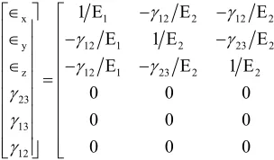
2.2. Compliance Matrix

In composite material fibers may be oriented in an arbi-trary manner. Depending on the arrangements of the fi-bers, the material may behave differently in different directions. According to their behaviour, composites may be characterized as generally anisotropic, monoclinic, orthotropic, and transversely isotropic. In this paper, transversely isotropic characteristics have been consid-ered for the fiber reinforced composite and fiber ar-rangement as shown in the Figure 1.

3

2

1

Figure 1. Arrangement of fiber direction for transversely sotropic composite.

i





x 1 12 2 12 2

y 12 1 2 23 2

z 12 1 23 2 2

23 23 2

13 12

12

1 E E E 0 0

E 1 E E 0 0

E E 1 E 0 0

0 0 0 2 1 E 0

0 0 0 0 1 G

0 0 0 0 0

23 13 12 12 0 0 0 0 0 1 G x y z                                                      _  _{ }                          

Here 1-2-3 orthogonal coordinate system is used where

the directions are taken as follows: _v

1 _dV

V

ij





 The 1-axis is aligned with the fiber direction.

3. Computational Details

 The 2-axis is in the plane of the layer and perpen-dicular to the fibers.

In this present work, finite element method is used to approximate the different elastic property of the fiber reinforced composites by ANSYS 12.

 The 3-axis is perpendicular to the plane of the layer and thus also perpendicular to the fibers.

Stress strain relationship for compliance matrix for

transversely isotropic matrix given below. Assumptions made for the present analysis were

 The composite is

♦Macroscopically homogeneous; 2.3. Representative Volume Element (RVE)

♦Linearly elastic; Primary to use of numerical approximations of the

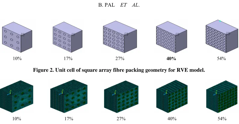
effec-tive properties of composite is the concept of representa-tive volume element (RVE). Square or cubic RVEs are used for most numerical approximations because of the ease of numerically solving boundary values problems with these geometries. The difficulties involved in gen-erating statistical information about particle distributions and concentrations leads to difficulties in the rigorous determination of RVE sizes. Hence, for most applications, RVE sizes have been rather arbitrary. In this paper a RVE model of 420 µm × 420 µm has considered which consists of different volume fraction of fiber density. In the model calculations, cuboid will be matrix and cylin-der will be fiber. Figure 2 shows the typical RVE which consists of 10%, 17%, 27%, 40% and 50% of fiber con-tent.

♦Macroscopically transversely isotropic; ♦Initially stress free (no thermal stress).

 The fibers are: ♦Homogeneous; ♦Linearly elastic; ♦Isotropic; ♦Regularly spaced; ♦Perfectly aligned.

 The matrix is: ♦Homogeneous; ♦Linearly elastic; ♦Isotropic.

3.1. Modelling

A regular three-dimensional arrangement of short fibre in a matrix was adequate to describe the overall behaviour of the composite, was modelled as a regular uniform ar-rangement, as shown in Figure 1. This model assumed that the fibre was a perfect cylinder of length 250 µm, and diameter (d = 50 µm) in a cube (420 × 420 × 250 µm3_{) of matrix. It is assumed that the geometry, material} and loading of the unit cell are symmetrical with respect to x-y-z coordinate system as shown in Figure 2. There-fore, 10% volume fraction i.e. 9 fibers has been inserted in a cubic matrix (420 × 420 × 250 µm3_{) uniformly as} shown in Figure 2. 3D finite element meshing for the 10% volume fraction of the fiber has been done, simi-larly the finite element modelling and meshing were done by varying the fiber volume fraction from 10% to 54% and as shown in Figure 3.

2.4. Homoginization

In classical lamination theory the composite lamina is modelled as a homogeneous orthotropic medium with certain effective moduli that describe the “average” ma-terial properties of the composite. To describe this mac-roscopically homogeneous medium, macro-stress and macro-strain are derived by averaging the stress and strain tensor over the volume of the RVE. The average stress and strain quantities defined in Equations (9) and (10) thus ensure equivalence in strain energy between the equivalent homogeneous material and the original het-erogeneous material. These average quantities will be used in the subsequent analysis to determine composite moduli

3.2. Element Type

v

1

dV

V ij

ij

_

10% 17% 27% 40% 54%

Figure 2. Unit cell of square array fibre packing geometry for RVE model.

10% 17% 27% 40% 54%

Figure 3. Finite element mesh for 10% volume fraction.

present analysis which is based on a general 3D state of stress and is suited for modeling 3D solid structure under 3D loading. The element has 8 noded brick element with three degrees of freedom per node (UX, UY and UZ).

3.3. Boundary Condition

In this work the boundary condition with normal strain applied in x direction are as follows [11]:

 

 





 

u LF 0, v BF 0, w BKF 0 and u RF 





x

x x

y

z

u 0, y,z 0

5.0E 05 0

onstant 0 constant

where LF, BF, BKF and RF stand for left face, bottom face, back face and right face of the RVE model. All other faces are free of any displacement.

In this paper, axial loading is modelled by a displace-ment acting on the plane yz at x. For such loading condi-tions, the boundaries of the RVE also correspond to lines of symmetry. Thus, normal displacements of the bounda-ries of the quadrant are restricted to those that cause the boundary to displace only parallel to the original bound-ary.

The displacement constraints applied to the finite ele-ment model to determine E1 are as follows and as shown in Figure 4.





















y y z z

u x, y,z u x,0,z

u x, y,z c

u x, y,0 u x, y,z









  

 

 





3.4. Material Property

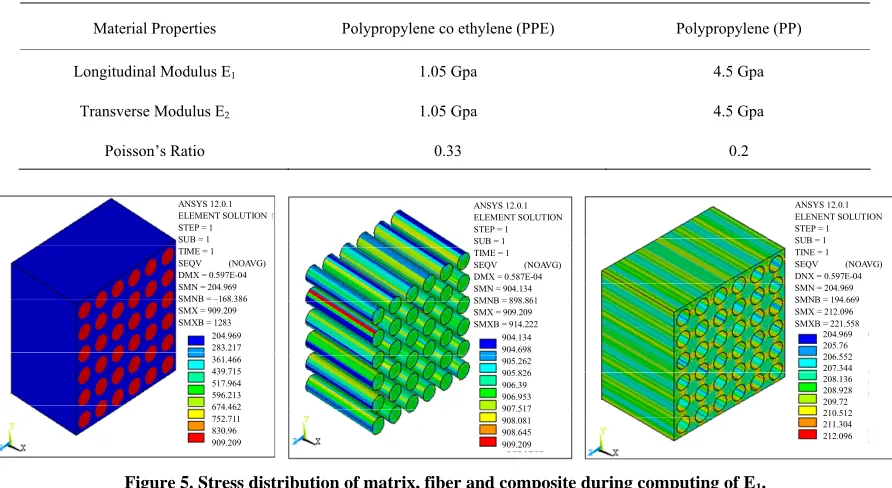
The different material properties of both matrix and fiber has shown in the Table 1.

Material properties are used to determine the several

elastic properties of the composite that is Longitudinal young’s modulus (E1) and Transverse young’s modulus (E2) by varying the volume fraction of the fiber.

3.5. Sample Analysis

Figure 5 shows the analysis of 40% of volume fraction of fiber reinforced composite in which the von misses stresses for the matrix fiber and composite has been in-dicated. The stresses are obtained by applying the dis-placement loading in longitudinal direction.

4. Results and Discussion

4.1. Longitudinal Young’s Modulus (E1)

Figure 6 shows comparison of finite element data, rule of mixtures and Halphin-Tasi results for composite mo- dulli E1 at different volume fractions. The finite-element solution gives identical results to the rule of mixtures and semi empirical analytical formulation. The linear de-pendence of E1 on fibre volume fraction is demonstrated and, as expected, the modulus increases while increasing the fibre volume fraction.

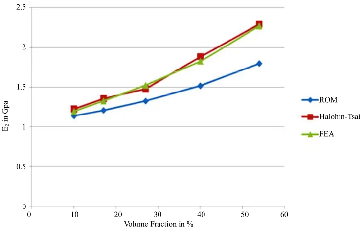
4.2. Transverse Young’s Modulus (E2)

Figure 7 shows comparison of finite element data, rule of mixtures and Halphin-Tasi results for composite mo- dulli E2 at different volume fractions. Finite element re-sults are as expected; on the assumption that the compos-ite is macroscopically transversely isotropic the values obtained for the whole unit cells investigated are per-fectly coincident. The Rule of mixtures model, the Hal-pin-Tsai equation and data from the finite-element cal-culations are compared. The term “ξ” is called the rein-forcing factor in Halpin Tsai equation and depends on the fiber geometry, packing geometry, loading condition. As he fibers are circular and packing density is increasing t

Figure 4. Boundary condition for longitudinal modulus of composite in x direction.

Table 1. Shows the material properties of composites.

Material Properties Polypropylene co ethylene (PPE) Polypropylene (PP)

Longitudinal Modulus E1 1.05 Gpa 4.5 Gpa

Transverse Modulus E2 1.05 Gpa 4.5 Gpa

Poisson’s Ratio 0.33 0.2

ANSYS 12.0.1 ELEMENT SOLUTION STEP = 1 SUB = 1 TIME = 1 SEQV (NOAVG) DMX = 0.597E-04 SMN = 204.969 SMNB = –168.386 SMX = 909.209 SMXB = 1283

204.969 283.217 361.466 439.715 517.964 596.213 674.462 752.711 830.96 909.209

ANSYS 12.0.1 ELEMENT SOLUTION STEP = 1 SUB = 1 TIME = 1 SEQV (NOAVG) DMX = 0.587E-04 SMN = 904.134 SMNB = 898.861 SMX = 909.209 SMXB = 914.222

904.134 904.698 905.262 905.826 906.39 906.953 907.517 908.081 908.645 909.209

ANSYS 12.0.1 ELENENT SOLUTION STEP = 1 SUB = 1 TINE = 1 SEQV (NOAVG) DNX = 0.597E-04 SMN = 204.969 SMNB = 194.669 SMX = 212.096 SMXB = 221.558

204.969 205.76 206.552 207.344 208.136 208.928 209.72 210.512 211.304 212.096

Figure 5. Stress distribution of matrix, fiber and composite during computing of E1.

ROM H-T Model FEA 3.5

3

2.5

2

1.5

1

0.5

0

0 10 20 30 40 50 60 Volume Fraction in %

E1

in

G

pa

Figure 6. Comparison of finite element data, rule of mixtures and Halphin-Tasi results for composite modulli E1 for different

ROM

Halohin-Tsai

FEA 2.5

2

1.5

1

0.5

0

0 10 20 30 40 50 60 Volume Fraction in %

E2

in

G

pa

Figure 7. Comparison of finite element data, rule of mixtures and Halphin-Tasi results for composite modulli E2 for different

volume fration of fiber.

accordingly the “ξ = 2” is adapted to consider those changes in the composites. In this Halpin-Tsai equation shows a good agreement between finite element values. But in Rule of mixture there is no such parameter which can be considered for those changes. Due to this reason The Rule of mixture is not showing the good agreement with finite element data.

4.3. Poisson’s Ratio

The major Poisson’s ratio 12 for the composite is de-fined as minus the ratio of strain in the y-direction di-vided by the strain in the x-direction when only the stress

x

 is applied. The Rule of Mixtures expression for the composite Poisson’s ratio is similar in form to the ex-pression for E1. It evident from the Figure 8 that ana-lytical and numerical results are in perfect agreement although data from the Rules of Mixtures are slightly higher than the finite-element results.

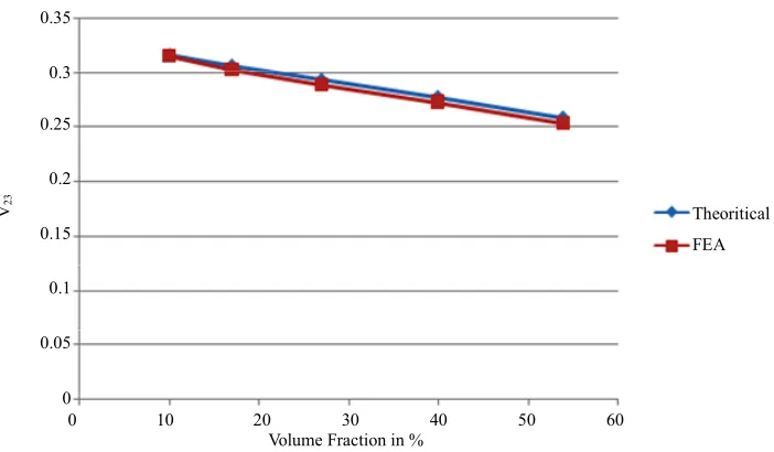
The Poisson’s ratio 23 describes the contraction in the z-direction on 23 applying loads in the y-direction. No analytical formulas have been applied to compare with numerical results of Poisson’s ratio. It is worthwhile to show finite element results of both with different fibre volume fractions. As expected from the Figure 9, 23 appears to be higher than 12 and the comparison be-tween the two Poisson’s ratios shows that Poisson’s ra-tios 12 are less sensitive to the fibre volume fraction. In particular, the values of 12 are quite close to the Poisson’s ratio of polypropylene (PP) especially at higher fibre volume fraction. On the contrary, 23 is strongly dependent from the fibre volume fraction and, its values

approaches the Poisson’s ratio of the Polypropylene co ethylene at lower values of the fibre volume fraction.

5. Conclusions

1) The 3D unit cell of the unidirectional fiber rein-forced composite has been identified (RVE) as a basic building block for estimating overall mechanical com-posite properties.

2) Various micromechanical methods to determine the elastic behaviour of composite materials have been dis-cussed.

3) Finite element analysis has provided an implicit means of modelling polymer composites.

4) Numerical homogenization tools have been devel-oped for the evaluation of the effective material proper-ties of the short fiber composites.

5) The appropriate constraints on the RVE under vari-ous loadings have been determined from symmetry boundary conditions, obtaining a nearly complete set of elastic constants for a three-dimensional unidirectional composite.

6) The results of elastic moduli E1, E2, E2, ν12, ν23, compared with the results of analytical solution and it is found that the results from FE simulation are in good agreement with the analytical results employed in this exercise namely the Halpin-Tsai semi-empirical expres-sion and to some extent the Rules of Mixtures.

7) As this mechanical property of fiber-filled compos-ites are affected by a number of parameters such as fiber type, matrix type, fiber orientation, fiber geometry, vol-ume fraction of the fibers and the degree of interfacial

Theoritical FEA 0.35

0.3

0.25

0.2

0.15

0.1

0.05

0

0 10 20 30 40 50 60 Volume Fraction in %

V23

Figure 8. Comparison of finite element data and rule of mixtures results for composite poisson’s ratio 12.

FEA.V12

FEA.V23

0.4

0.35

0.3

0.25

0.2

0.15

0.1

0.05

0

0 10 20 30 40 50 60 Volume Fraction in %

V12

an

d

V23

Figure 9. Comparison of finite element results for composite poisson’s ratio 12 and 23.

adhesion between the fiber and the polymer matrix, the ROM has not been adopted by this property expect the volume fraction. So the results are also not so accurate.

8) The Halpin-Tsai (HT) model is also a theoretical model. This model, besides the modulus of elasticity of the polymer, Em, and of the fiber, Ef, includes a geomet- rical parameter (aspect ratio) of the fiber as well. The model has a complicated mathematical structure with fiber geometry, packing geometry, loading condition. This factors help to showing the good agreement with finite element data.

9) It is observed that the change in volume fraction of fiber has a significant effect on elastic properties.

REFERENCES

[1] D. F. Adams and D. R. Doner, “Longitudinal Shear

Load-ing of a Unidirectional Composite,” Journal Composite Materials, Vol. 1, No. 1, 1967, pp. 4-17.

[2] D. F. Adams and D. R. Doner, “Transverse Normal Load- ing of a Unidirectional Composite,” Journal Composite Materials, Vol. 1, No. 2, 1967, pp. 152-164.

doi:10.1177/002199836700100205

[3] S. Houshyar, R. A. Shanks and A. Hodzic, “Modelling of Polypropylene Fibre-Matrix Composites Using Finite Ele- ment Analysis,” Express Polymer Letters, Vol. 13, No. 1, 2009, pp. 2-12.

[4] S. Houshyar, R. A. Shanks and A. Hodzic, “The Effect of Fibre Concentration on Mechanical and Thermal Proper- ties of Fibre Reinforced Polypropylene Composites,” Jour- nal of Applied Polymer Science, Vol. 96, No. 6, 2005, pp. 2260-2272. doi:10.1002/app.20874

of Materials Science, Vol. 32, No. 16, 1999, pp. 4261- 4267. doi:10.1023/A:1018651218515

[6] C. T. Sun and R. S. Vaidya, “Prediction of Composite Properties from a Representative Volume Element,” Com- posites Science and Technology, Vol. 56, No. 2, 1996, pp. 171-179. doi:10.1016/0266-3538(95)00141-7

[7] S. Li, “General Unit Cell for Micromechanical Analyses of Unidirectional Composites,” Composites Part A, Vol. 32, No. 6, 2000, pp. 815-816.

doi:10.1016/S1359-835X(00)00182-2

[8] B. R. Kim and H. K. Lee, “An RVE-Based Microme-

chanical Analysis of Fiber-Reinforced Composites Con- sidering Fiber Size Dependency,” Composite Structures, Vol. 90, No. 4, 2009, pp. 418-427.

doi:10.1016/j.compstruct.2009.04.025

[9] P. De Buhan and A. Taliercio, “A Homogenisation Ap-

proach to the Yield Strength of Compositematerials,” Eu- ropean Journal of Mechanics, Vol. 10, No. 2, 1991, pp. 129-154.

[10] Y. Pan, L. Iorga and A. A. Pelegri, “Numerical Genera- tion of a Random Chopped Fiber Composite RVE and Its Elastic Pproperties,” Composites Science and Technology,

Vol. 68, No. 13, 2008, pp. 2792-2798. doi:10.1016/j.compscitech.2008.06.007

[11] M. Porfiri and N. Gupta, “Effect of Volume Fraction and Wall Thickness on the Elastic Properties of Hollow Parti- cle Filled Composites,” Composites Part B: Engineering, Vol. 40, No. 2, 2009, pp. 166-173.

doi:10.1016/j.compositesb.2008.09.002

[12] K. Hbaieb, Q. Wang, Y. H. J. Chia and B. Cotterell, “Mo- delling Stiffness of Polymer/Clay Nanocomposites,” Po- lymer, Vol. 48, No. 3, 2007, pp. 901-909.

doi:10.1016/j.polymer.2006.11.062

[13] A. G. Facca, M. T. Kortschot and N. Yan, “Predicting the Elastic Modulus of Natural Fibre Reinforced Thermo- plastics,” Composites Part A: Applied Science and Manu- facturing, Vol. 37, No. 10, 2006, pp. 1660-1671. doi:10.1016/j.compositesa.2005.10.006

[14] L. Peponi, J. Biagiotti, J. M. Kenny and I. Mondragon, “Statistical Analysis of the Mechanical Properties of Na- tural Fibers and Their Composite Materials. II. Composite Materials,” Polymer Composites, Vol. 29, No. 3, 2008, pp. 321-325. doi:10.1002/pc.20386