Effects of wing deformation on aerodynamic forces in hovering hoverflies

INTRODUCTION

The flight mechanics of small insects is gaining more attention than before due to possible applications in micro-flying-machines. In recent years, much work has been done on the flapping insect wing using experimental and computational methods (e.g. Ellington et al., 1996; Dickinson et al., 1999; Usherwood and Ellington, 2002a; Usherwood and Ellington, 2002b; Sane and Dickinson, 2001; Liu et al., 1998; Sun and Tang, 2002; Wang et al., 2004), and considerable understanding of the aerodynamic force generation mechanism has been achieved.

However, in most of these studies, rigid model wings were employed. Observations of free-flying insects have shown that wing deformations (time-varying camber and spanwise twist) are present (e.g. Ellington, 1984b; Ennos, 1989). How does the time-varying wing deformation affect the aerodynamic forces on the flapping wings compared with that of a rigid model wing? Studies of this problem are very limited. In their experiment investigating the leading edge vortex, Ellington et al. modeled wing deformation through low-order camber changes in the model-wing of the hawkmoth (Ellington et al., 1996), but did not test the corresponding rigid model wing for comparison. Du and Sun conducted a computational study on this problem and showed that the deformation did indeed have some effects on the aerodynamic forces (Du and Sun, 2008). By removing the camber and the spanwise twist one by one, they also showed that it was the camber that played the major role in affecting the aerodynamic force. However, in their study, the authors assumed that (1) the camber and twist increased from zero to some constant value at the beginning of a half-stroke (downstroke or upstroke) and kept a constant value in the mid portion of the half-stroke and (2) in the later part of the half-stroke, the camber and twist started to decrease and became zero at the end of

the half-stroke. This time variation of wing deformation was based on Ellington’s and Ennos’ qualitative descriptions of wing motion in hovering insects filmed using one high-speed camera (Ellington, 1984b; Ennos, 1989). Recently, using four high-speed digital video cameras, Walker et al. obtained quantitative data on the time-varying camber and spanwise twist of wings in free-flying droneflies (Walker et al., 2009).

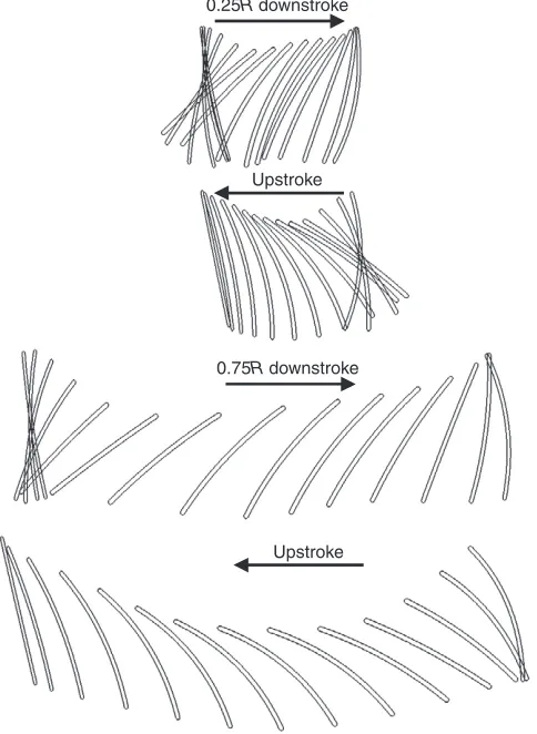
These data showed that camber and twist were approximately constant in the mid half-stroke, similar to that described by Ellington and Ennos (Ellington, 1984b; Ennos, 1989); but, around the stroke reversal, unlike that described by Ellington and Ennos, the camber and twist were much larger than that in the mid half-stroke. Fig.1 gives the diagrams of wing motion showing the instantaneous wing profiles at two distances along the wing length in one half-stroke (upstroke) used by Du and Sun (Fig.1A), compared with that measured by Walker et al. (Du and Sun, 2008; Walker et al., 2009) (Fig.1B). It can be seen that the wing deformations in Du and Sun’s study are rather different from the measured one. Furthermore, in the Du and Sun paper, the camber value was arbitrarily assumed. Recently, Zhao et al. conducted an experimental study on the aerodynamic effects of flexibility in flapping wings (Zhao et al., 2010). Using model wings with various flexural stiffness and a simple framework of wing veins, they showed that flexible wings could generate forces nearly the same or even higher than the rigid model wing. But, similar to Du and Sun’s work (Du and Sun, 2008), the deformation was ‘assumed’ in this study. It is therefore of great interest to study the aerodynamic effects of wing deformation using realistic data.

In the present work, we study the aerodynamic forces and aerodynamic power requirements of the deformable wing of the hoverflies in the experiment of Walker et al. (Walker et al., 2009), The Journal of Experimental Biology 213, 2273-2283

© 2010. Published by The Company of Biologists Ltd doi:10.1242/jeb.040295

Effects of wing deformation on aerodynamic forces in hovering hoverflies

Gang Du* and Mao Sun

Ministry-of-Education Key Laboratory of Fluid Mechanics, Beijing University of Aeronautics and Astronautics, Beijing, China *Author for correspondence ([email protected])

Accepted 30 March 2010

SUMMARY

We studied the effects of wing deformation on the aerodynamic forces of wings of hovering hoverflies by solving the Navier–Stokes equations on a dynamically deforming grid, employing the recently measured wing deformation data of hoverflies in free-flight. Three hoverflies were considered. By taking out the camber deformation and the spanwise twist deformation one by one and by comparing the results of the deformable wing with those of the rigid plate wing (the angle of attack of the rigid flat-plate wing was equal to the local angle of attack at the radius of the second moment of wing area of the deformable wing), effects of camber deformation and spanwise twist were identified. The main results are as follows. For the hovering hoverflies considered, the time courses of the lift, drag and aerodynamic power coefficients of the deformable wing are very similar to their counterparts of the rigid flat-plate wing, although lift of the deformable wing is about 10% larger, and its aerodynamic power required about 5% less than that of the rigid flat-plate wing. The difference in lift is mainly caused by the camber deformation, and the difference in power is mainly caused by the spanwise twist. The main reason that the deformation does not have a very large effect on the aerodynamic force is that, during hovering, the wing operates at a very high angle of attack (about 50deg) and the flow is separated, and separated flow is not very sensitive to wing deformation. Thus, as a first approximation, the deformable wing in hover flight could be modeled by a rigid flat-plate wing with its angle of attack being equal to the local angle of attack at the radius of second moment of wing area of the deformable wing.

using the data of realistic wing deformation, by numerically solving the Navier–Stokes equations on a dynamically deforming grid. The results are compared with those of a rigid flat-plate wing, the angle of attack of which was equal to the local angle of attack at the radius of the second moment of wing area of the deformable wing. The comparison shows the effects of the wing deformation on the aerodynamic forces and moments and also tells us how well a rigid flat-plate wing could model the deformable wing.

MATERIALS AND METHODS

Governing equations and the solution method The governing equations employed in this study are the unsteady three-dimensional incompressible Navier–Stokes equations:

 u0 , (1)

where uis the fluid velocity, pis the pressure, is the density, v

is the kinematic viscosity, is the gradient operator and 2_{is the} Laplacian operator.

Eqns 1 and 2 are solved numerically, and a dynamically deforming grid is used to treat the time-variant deformation of the wing. The solution method and the method to generate the dynamically deforming grid have been described in detail by Du and Sun (Du and Sun, 2008), and so only an outline of the methods is given here. Eqns 1 and 2 are solved using an algorithm based on

∂u

∂t +u⋅ ∇u=− 1

ρ∇p v+ ∇2u , (2)

the method of artificial compressibility (Rogers and Kwak, 1990; Rogers et al., 1991), which has the advantage of solving the incompressible fluid flows using the well-developed methods for compressible fluid flows. A procedure of combining the method of the modified trans-finite interpolation (Morton et al., 1998) and the

0.25R

0.75R

0.25R

0.75R

A

B

Fig.1. Diagram of wing motion in the upstroke showing the instantaneous wing profiles of 25% and 75% wing length (R). (A) wing motion used by Du and Sun (Du and Sun, 2008); (B) wing motion redrawn using Walker et al.’s data (Walker et al., 2009).

Wing root

Axis of pitching rotation

A

B

Z X

Y

R

O

α

θ

φ

Fig.2. (A) Wing planform used. (B) A sketch showing the stroke plane and the definitions of the wing kinematic parameters (see List of Symbols and Abbreviations).

Upstroke

0.75R downstroke 0.25R downstroke

Upstroke

method of solving Poisson equation is used to generate the dynamically deforming grid. For far-field boundary conditions, at the inflow boundary, the velocity components are specified as free-stream conditions while the pressure is extrapolated from the interior; at the outflow boundary, the pressure is set to be equal to the free-stream static pressure and the velocity is extrapolated from the interior. On the airfoil surfaces, impermeable wall and no-slip boundary conditions were applied, and the pressure on the boundary is obtained from the normal component of the momentum equation.

The wing, wing motion and wing deformation

The planform of the wing used in the present study is approximately the same as that of a hoverfly wing, with small parts of the wing tip and wing base cut off (Fig.2A). Without the cut-off, the wing tip (and wing base) would be much narrower than the middle portion of the wing, and the computational grid near the tip and the base would have large distortion, which would make the computation less accurate. When the wing has large deformation, the distortion could be even more severe. Therefore, small parts of the wing base and wing tip are cut off (the length of the cut-off wing tip is only 3.3% of the wing length). The location of the wing root (i.e. the point about which the wing rotates) and the location of the axis of pitching rotation (the line joining the wing tip and the wing root) are determined before the cut-off. They, and hence the wing motion, will not be affected by the cut-off. The wing shape is changed a little by the cut-off, but since the same modified wing is used for

both the case with deformation and the case without deformation, it is expected that this modification would not affect our study of the effect of deformation. The wing section is a flat plate of 3% thickness with rounded leading and trailing edges.

The wing motion and wing deformation are prescribed on the basis of the measured data by Walker et al. (Walker et al., 2009). As discussed in Walker et al.’s paper, the wing motion and deformation could be determined in terms of the wing-tip kinematics, the local angle of attack of each wing section (), and the camber of each wing section. Walker et al. measured the relevant quantities for five free-flying hoverflies. How each of these quantities is modeled is discussed in the following.

First, we consider the wing-tip kinematics, which is determined by the stroke angle () and the deviation angle () (Fig.2A). Walker et al. gave data on the time courses of and [see fig.1 of Walker et al. (Walker et al., 2009)]. In the present study, we use the first six terms of the Fourier series to fit the data and obtain the time courses of and .

Next, we consider the local angle of attack of each wing section. Walker et al. showed that the wing had an approximate linear spanwise twist [see fig.5 of Walker et al. (Walker et al., 2009)]. They gave data on the time course of at 50% of wing length [see fig.4 of Walker et al. (Walker et al., 2009)], together with data on the time course of twist angle [see fig.6A of Walker et al. (Walker et al., 2009)]. We fit the data using the first six terms of the Fourier series to obtain the time courses of at 50% wing length and the

–2 0 2 4 6

–4 –2 0 2 4 6

Rigid flat-plate wing Deformable wing

CP,

a

CD

0.2

0 0.4 0.6 0.8 1.0

0

3

6 9

tˆ

C

B

A

CL

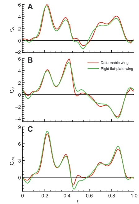
Fig. 4. Time courses of the (A) lift (CL), (B) drag (CD) and (C) power (CP,a) coefficients of the deformable wing in one cycle, compared with those of the rigid flat-plate wing, for hoverfly H3. t, non-dimensional time.

0 2 4 6

–4 –2 0 2 4 6

Spanwise twist only Camber only Rigid flat-plate wing

0

3

6 9

C

B

A

CP,

a

CD

0.2

0 0.4 0.6 0.8 1.0

CL

tˆ

twist angle. Since the wing has linear spanwise twist, the time course of for each wing section can be obtained.

Finally, we consider the wing camber. Walker et al. gave data on the time course of wing camber at 50% wing length [see fig.9C,F in Walker et al. (Walker et al., 2009)]. They also gave data on the spanwise distribution of camber at mid down- and upstrokes. We

assume that the spanwise distribution of camber at the mid half-stroke could represent that at other times of the half-stroke. With this assumption and with the time course of camber at 50% wing length (obtained by fitting the data using the first six terms of the Fourier series), the time course of camber of each wing section is obtained. As an example, Fig.3 gives the diagram of wing motion for hoverfly H3, showing its instantaneous wing profile at two distances along the wing in one wingbeat cycle.

RESULTS AND DISCUSSION

The flow solver has been tested by Du and Sun using two sets of computations (Du and Sun, 2008). First, they tested the flexible grid method. Flows of a rigid model wing in flapping motion were computed in two ways: rigid grid motion, in which the whole grid system moved with the wing, and flexible grid motion, in which the far boundary of the grid was fixed and the inner grid was deformed as the wing moved. Results of these two calculations were almost identical, as they should be. Second, they tested the solver against Usherwood and Ellington’s experimental data of a model bumblebee wing in revolving motion (Usherwood and Ellington, 2002a). Results of the solutions agreed with the experimental data. These cross-validations gave overall confidence in the solver and the dynamically deforming grid. Du and Sun also made grid resolution tests for the wing for cases with Reynolds number (Re) ranging from 200 to 4000 and showed that grid dimensions of 109⫻90⫻120 and an outer boundary at 30 wing chord length from the wing were proper to resolve the flow (Du and Sun, 2008) [Re

is defined as: ReUc/v, where vis the kinematic viscosity, cis the mean chord length of the wing and Uis the reference speed, defined as U2nr2, where is the stroke amplitude (max–min), nis the wingbeat frequency and r2is the radius of the second moment of wing area]. In the present study, Reis approximately 800, and the above grid dimension should be proper to resolve the flow, and so these grid dimensions are used.

–2 0 2 4

–2 0 2 4

Rigid flat-plate wing Deformable wing

–2 0 2 4 6

C

B

A

CP,

a

CD

0.2

0 0.4 0.6 0.8 1.0

CL

tˆ

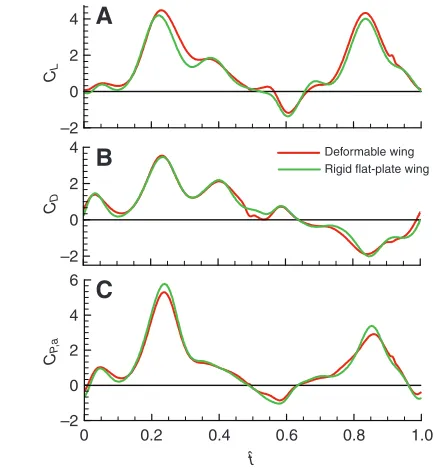
Fig. 6. Time courses of the (A) lift (CL), (B) drag (CD) and (C) power (CP,a) coefficients of the deformable wing in one cycle, compared to those of the rigid flat-plate wing, for hoverfly H4. t, non-dimensional time.

–2 0 2 4

–2 0 2 4

Spanwise twist only Camber only Rigid flat-plate wing

–2 0 2 4 6

C

B

A

CP,

a

CD

0.2

0 0.4 0.6 0.8 1.0

CL

tˆ

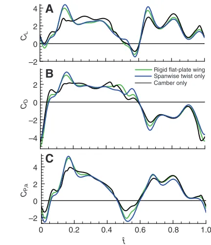
Fig. 7. Time courses of the (A) lift (CL), (B) drag (CD) and (C) power (CP,a) coefficients of the wing with spanwise twist only and the wing with camber only in one cycle, compared with those of the rigid flat-plate wing, for hoverfly H4. t, non-dimensional time.

–2

Rigid flat-plate wing Deformable wing

0 2

–4 –2 0 2

–2 0 2 4 4

C

B

A

CP,

a

CD

0.2

0 0.4 0.6 0.8 1.0

CL

tˆ

Three of the five hoverflies considered by Walker et al. (Walker et al., 2009) are chosen for the present analysis (they are hoverflies H3, H4 and H5 from Walker et al.’s study). , n, R(wing length) andm(mass of the insect) of hoverflies H3, H4 and H5 are listed in Table1 (taken from Walker et al., 2009). Ellington measured R,

r2and cof hoverflies in his study and gave: r2/R⬇0.56, c/R⬇0.28 (Ellington, 1984a). We assume that the ratios, r2/Rand c/R, are approximately the same for different individuals, and r2/R⬇0.56

and c/R⬇0.28 are used for the three insects considered here. Thus,

r2and cor S(wing area) become known for the insects, and they are also listed in Table1.

CL, CD and CP,a denote the coefficients of lift, drag and

aerodynamic power required of the wing, respectively; the lift and drag are non-dimensionalized by 0.5U2_{S, and the aerodynamic} power required is non-dimensionalized by 0.5U3_Sc.

The effects of wing deformation on the aerodynamic forces For a clear description of the results, we express the time during a cycle as a non-dimensional parameter, t, such that t0 at the start of a downstroke and t1 at the end of the subsequent upstroke. Fig.4 gives the time courses of CL, CDand CP,aof the deformable wing

in one cycle; results for the rigid flat-plate wing are included for comparison (note that the rigid flat-plate wing has the same angle of attack as that of the wing section at r2of the deformable wing). It is seen that the time courses of CL, CDand CP,aof the deformable

wing are very similar to their counterparts of the rigid flat-plate wing, although CLand CDof the deformable wing are a little larger,

and CP,ais a little smaller, than those of the rigid flat-plate wing.

The mean lift (CL), drag (CD) and aerodynamic power (CP,a)

coefficients for dronefly H3 are given in Table2. It is seen that CL

and CDof the rigid flat-plate wing are about 10% and 4% smaller,

and CP,a is about 5% larger, than those of the deformable wing,

respectively.

To isolate the effects of wing camber and wing twist, we make two more calculations for hoverfly H3: (1) the wing camber is made zero and only the spanwise twist exists and (2) the spanwise twist is made zero and only the camber deformation exists. The results, compared with those of the rigid flat-plate wing, are shown in Fig.5.

–2 0 2 4

–4 –2 0 2

–2 0 2 4

C

B

A

Rigid flat-plate wing

Spanwise twist only Camber only

CP,

a

CD

0.2

0 0.4 0.6 0.8 1.0

CL

tˆ

Fig. 9. Time courses of the (A) lift (CL), (B) drag (CD) and (C) power (CP,a) coefficients of the wing with spanwise twist only and the wing with camber only in one cycle, compared with those of the rigid flat-plate wing, for hoverfly H5. t, non-dimensional time.

0 4 8 12

Camber only Rigid flat-plate wing

Rigid flat-plate wing Spanwise twist only

r/R Cd

Cl

0.5 0

4 8

1

i

ii

0.5 1

i

ii

A

B

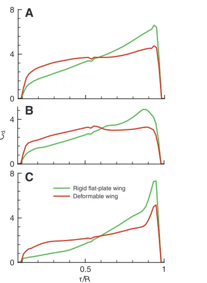
Fig. 10. Spanwise lift and drag distributions at mid-downstroke of the wing with camber deformation only (A) and of the wing with spanwise twist deformation only (B) for hoverfly H3, compared with that of the rigid flat-plate wing. Cland Cd, non-dimensional lift and drag per unit wing length, respectively;r, radial position along wing length; R, wing length.

0 4 8

Camber only Rigid flat-plate wing

Rigid flat-plate wing Spanwise twist only

0 4

r/R Cd

Cl

0.5 1

i

ii

0.5 1

i

ii

A

B

Fig. 11. Spanwise lift and drag distributions at mid-downstroke of the wing with camber deformation only (A) and of the wing with spanwise twist deformation only (B) for hoverfly H4, compared with that of the rigid flat-plate wing. Cland Cd, non-dimensional lift and drag per unit wing length, respectively;r, radial position along wing length; R, wing length.

Table 1. Flight data

m* * R* n* S c r2

I.D. (mg) (deg) (mm) (Hz) (mm2_{) (mm) (mm)}

H3 125 91.8 12.4 152 43.03 3.47 6.94

H4 181 116.1 12.6 180 44.48 3.53 7.06

H5 108 105.8 12.3 149 42.31 3.44 6.89

The corresponding CL, CDand CP,aare also given in Table2. It is

seen that the aerodynamic forces of the wing with spanwise twist only are very close to those of the rigid flat-plate, but the aerodynamic forces of the wing with camber only are a little different from those of the rigid flat-plate. This shows that the wing camber plays a major role in causing the differences in the aerodynamic forces between the deformable wing and the rigid flat-plate wing.

The same computations as those made for hoverfly H3 are made for hoverflies H4 and H5. The time courses of CL, CDand CP,aof

hoverfly H4 are given in Fig.6 and Fig.7, and those of hoverfly H5 in Fig.8 and Fig.9. The corresponding mean force and power coefficients are also given in Table2. From Fig.6, Fig.8 and Table2, it is seen that for hoverflies H4 and H5, similar to the case of hoverfly H3, the time courses of CL, CDand CP,aof the deformable wing are

similar to those of the rigid flat-plate wing, although CLand CDof

the deformable wing are a little larger and CP,a is a little smaller

than those of the rigid flat-plate wing.

The result that camber deformation increases the aerodynamic forces is expected because camber can increase the asymmetry of the flows on the upper and lower surfaces of the wing. The result that the spanwise twist has very small effect on the aerodynamic forces is explained as follows. For the wing with spanwise twist, 

at r>r2is smaller than that of the flat-plate wing (rdenotes the radial position along the wing length) and at r<r2is larger than that of the flat-plate wing. Since the aerodynamic force is approximately proportional to , its aerodynamic force at r>r2would be larger than that of the flat-plate wing and its aerodynamic force at r<r2 would be smaller than that of the flat-plate wing. Thus, it is expected

that the aerodynamic force of the wing with spanwise twist is not very different from that of the flat-plate wing. These can be seen by comparing spanwise lift and drag distribution plots for midstroke when dynamic pressure and force are maximal. Fig.10A compares the lift and drag distribution plots at mid-downstroke between the wing with camber only and the rigid flat-plate wing for hoverfly H3, and Fig.10B compares the corresponding results between the wing with spanwise twist only and the rigid flat-plate wing. For the wing with camber only (Fig.10A), the aerodynamic forces are a little larger than those of the rigid flat-plate wing along the whole wing span, but for the wing with twist only (Fig.10B), in the outer part of the wing, the aerodynamic forces are larger than those of the rigid flat-plate wing, and in the inner part of the wing the opposite is true. The same comparisons are made for hoverflies H4 and H5 in Fig.11 and Fig.12, respectively, and similar results are observed. As seen in Table2, CDof the deformable wing is approximately

4% larger than that of the rigid flat-plate wing. One might expect that its aerodynamic power would be a little larger than that of the rigid flat-plate wing. However, results in Table2 show that CP,aof 0

4

8 Camber only Rigid flat-plate wing

Rigid flat-plate wing Spanwise twist only

0 4 8

r/R Cd

Cl

0.5 1

i

ii

0.5 1

i

ii

A

B

Fig. 12. Spanwise lift and drag distributions at mid-downstroke of the wing with camber deformation only (A) and of the wing with spanwise twist deformation only (B) for hoverfly H5, compared with that of the rigid flat-plate wing. Cland Cd, non-dimensional lift and drag per unit wing length, respectively;r, radial position along wing length; R, wing length.

0 4

8

0 4

0 4

8

Rigid flat-plate wing Deformable wing

C

B

A

r/R

Cd

0.5 1

Fig.13. Spanwise drag distribution at mid-downstroke of the deformable wing, compared with that of the rigid flat-plate wing, for hoverfly H3 (A), H4 (B) and H5 (C). Cd, non-dimensional drag per unit wing length; r, radial position along wing length; R, wing length.

Table 2. Mean aerodynamic force and power coefficients

CL CD CP,a

I.D. A B C D A B C D A B C D

H3 1.81 1.63 1.62 1.81 1.62 1.56 1.44 1.71 2.16 2.23 2.12 2.28

H4 1.38 1.19 1.17 1.39 1.07 1.04 0.97 1.10 1.29 1.33 1.22 1.39

H5 1.78 1.68 1.70 1.78 1.28 1.24 1.20 1.32 1.73 1.89 1.79 1.82

tˆ=0

tˆ=0.3 tˆ=0.4

tˆ=0.9

tˆ=0.8 tˆ=0.5

tˆ=0

tˆ=0.3

tˆ=0.4

tˆ=0.9 _tˆ=0.8 tˆ=0.5

tˆ=0

tˆ=0.3

tˆ=0.4

tˆ=0.9 _tˆ=0.8 tˆ=0.5

A

B

C

tˆ=0 _tˆ=0.3

tˆ=0.4

tˆ=0.9 _tˆ=0.8

tˆ=0.5

D

tˆ=0

tˆ=0.3

tˆ=0.4

tˆ=0.9

tˆ=0.8

tˆ=0.5

tˆ=0

tˆ=0.3

tˆ=0.4

tˆ=0.9 tˆ=0.8

tˆ=0.5

tˆ=0 tˆ=0.3

tˆ=0.4

tˆ=0.9

tˆ=0.8

tˆ=0.5

A

B

C

tˆ=0

tˆ=0.3

tˆ=0.4

tˆ=0.9

tˆ=0.8

tˆ=0.5

D

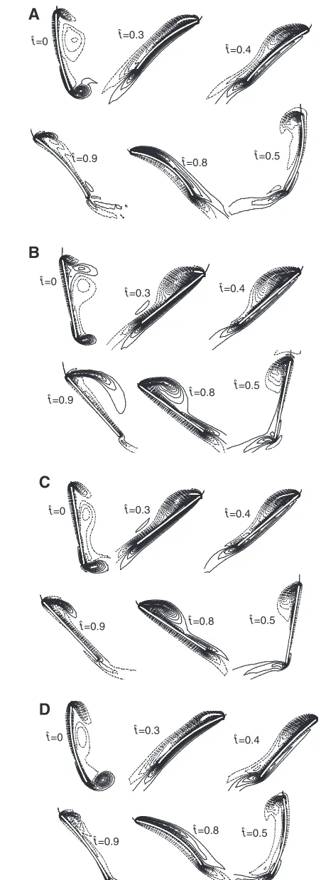
Fig. 14. Vorticity plots at 60% wing length at various times during one cycle for hoverfly H3. (A) deformable wing; (B) rigid flat-plate wing; (C) wing with twist only; (D) wing with camber only. Solid and broken lines indicate positive and negative vorticity, respectively; the magnitude of the non-dimensional vorticity at the outer contour is 2 and the contour interval is 3.

the deformable wing is a little smaller than that of the flat-plate wing. This is due to the effect of spanwise twist in the deformable wing. As observed above (Fig.10B, Fig.11B and Fig.12B), the spanwise twist can make the drag larger in the inner part of the wing and smaller in the outer part of the wing compared with the rigid flat-plate wing. This can reduce its torque of the drag force and hence the aerodynamic power. Fig.13A–C compares the spanwise drag distribution plot of the deformable wing at mid-downstroke with those of the rigid flat-plate wing for hoverflies H3, H4 and H5, respectively. It is clearly seen that the drag of the deformable wing in the inner part of the wing is larger, and in the outer part of the wing is smaller, than that of the rigid flat-plate wing.

The flow fields

Here, we use the flow information to gain further insights on the effects of wing deformation. Fig.14 shows the sectional vorticity contour plots at 60% wing length at various times in one cycle for the deformable wing of hoverfly H3 and the corresponding rigid flat-plate wing, wing with spanwise twist only, and wing with camber only.

We first compare the vorticity plots of the deformable wing (Fig.14A) with those of the rigid flat-plate wing (Fig.14B). Flow patterns of the two wings are qualitatively the same: both are dominated by the leading edge vortex (LEV). But there exist some differences between the LEVs of the two wings: the LEV of the deformable wing is a little more concentrated and a little closer to the wing surface than that of the rigid flat-plate wing. Vortex theory for aerodynamic force (Wu, 1981) shows that the aerodynamic force on the wing is proportional to the time rate of change of the total first moment of vorticity. For the flapping wing, the vorticity moment produced by a downstroke or upstroke is mainly determined by the vorticity in the LEV and the vorticity (of opposite sign to that of the LEV) in the trailing edge vortex. As the wing is translating, the vorticity shed from the trailing edge stays approximately at the place where it is shed, and the vorticity in the LEV moves almost at the same speed as that of the wing (Sun and Wu, 2004). This would produce a time rate of change of the vortex moment or aerodynamic force. When the LEV is more concentrated and closer to the wing, the time rate of change of the vorticity moment could be larger, i.e. the aerodynamic force on the wing could be larger.

Next, we compare the vorticity plots of the wing with spanwise twist only (Fig.14C) with those of the rigid flat-plate wing (Fig.14B). It is seen that the LEV of the wing with spanwise twist only is very close to that of the rigid flat-plate wing. This explains qualitatively why the aerodynamic force of the wing with spanwise twist only is very close to that of the rigid flat-plate wing.

Finally, we compare the vorticity plots of the wing with camber only (Fig.14D) with that of the deformable wing (Fig.14A). The LEV of the wing with camber only is very close to that of the deformable wing, qualitatively explaining why the lift of the deformable wing is very close to that of the wing with camber only. The same comparisons of vorticity plots are made for hoverflies H4 and H5 (Fig.15 and Fig.16, respectively) and in general the results are similar to that of hoverfly H3.

It is interesting to note that for some hoverflies, at a certain phase of the wingbeat cycle, the LEV has a double vortex structure (e.g. for hoverfly H3 at t0.3, Fig.14A; for hoverfly H4 at t0.3–0.5, Fig.15A). This phenomenon has been observed by Lu et al. in their flow visualization experiments on a flapping model dragonfly wing (Lu et al., 2006).

The effects of wing deformation on hovering efficiency Although the mean aerodynamic power coefficient (CP,a) of the rigid

flat-plate wing is only a little (about 5%) larger than that of the deformable wing (Table2), its mean lift coefficient (CL) is around

10% smaller than that of the deformable wing. This means that there could be a relatively large difference in aerodynamic power required for producing unit lift, which is a more relevant index for hovering performance, between the deformable wing and the rigid flat-plate and wing.

This power index is computed and shown in Table3. It is seen that aerodynamic power required for producing unit lift of the rigid flat-plate wing is about 17% higher than that of the deformable wing (for the wing with spanwise twist only and the wing with camber only, the number is 10% and 6%, respectively). These results show that the real deformable wing has the best hovering performance; when the camber is retained but the spanwise twist taken out, the performance becomes a little worse (power requirement becomes 6% higher); when the spanwise twist is retained but the camber taken out, the performance becomes worse to a larger extent (power requirement 10% higher); when the camber and spanwise twist are both taken out, i.e. for the rigid flat-plate wing, the performance is worst (power requirement 17% higher).

Recently, Young et al. did a similar computational study for locusts in forward flight (Young et al., 2009). Their results show that the power required per unit lift for the rigid flat-plate wing (1.96WN–1_{) and that for the wing with spanwise twist only} (1.28WN–1_{) are 41% and 12% higher than that of the deformable} wing (1.14WN–1_{), respectively. These numbers clearly show that,} in forward flight, the spanwise twist may play a much more

Table 3. Aerodynamic power required for producing unit lift (W N–1₎

I.D. A (deformable wing) B (flat-plate) C (twist only) D (camber only)

H3 4.04 4.64 4.44 4.27

H4 4.81 5.76 5.37 5.15

H5 3.68 4.26 3.99 3.88

A, deformable wing; B, rigid flat-plate wing; C, wing with twist deformation only; D, wing with camber deformation only.

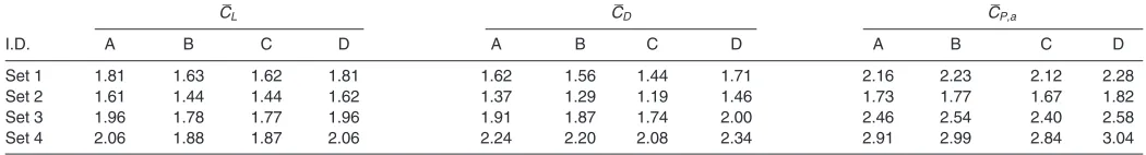
Table 4. Mean aerodynamic force and power coefficients for hoverfly H3 at different angles of attack at r2

CL CD CP,a

I.D. A B C D A B C D A B C D

Set 1 1.81 1.63 1.62 1.81 1.62 1.56 1.44 1.71 2.16 2.23 2.12 2.28

Set 2 1.61 1.44 1.44 1.62 1.37 1.29 1.19 1.46 1.73 1.77 1.67 1.82

Set 3 1.96 1.78 1.77 1.96 1.91 1.87 1.74 2.00 2.46 2.54 2.40 2.58

Set 4 2.06 1.88 1.87 2.06 2.24 2.20 2.08 2.34 2.91 2.99 2.84 3.04

important rote in improving the flight performance than in hovering.

Comparison of the computed lift with insect weight Walker et al. measured the mass of the hoverflies in their study (Walker et al., 2009). The non-dimensional weight, defined as

mg/0.5U2_{(2S), can be determined for droneflies in the present study.} The non-dimensional weights are 1.94, 1.21 and 1.46 for droneflies H3, H4 and H5, respectively.

As seen in Table2, the mean lift coefficients computed using the flow solver are 1.81, 1.38 and 1.78, respectively. The computed mean lift is about 10% smaller or larger than the insect weight, showing that the computational model is reasonably accurate.

Some discussions on modeling the wing as a rigid flat-plate In experimental and computational modeling of insect flapping wings, if the effects of wing deformation are to be included, the elastic property of the wing must be incorporated into the wing model. It is difficult to measure the elastic property of the wing of an insect in free-flight conditions (the elastic property of a wing cut off from the insect could be different from that of the live one operating during flight). Therefore, it is of great interest to know how well a rigid flat-plate wing can model the real wing.

The above results show that the time courses of the force and aerodynamic power coefficients (CL, CDand CP,a) of the deformable

wing are very similar to those of the rigid flat-plate wing (the angle of attack of the flat-plate wing being equal to the local angle of attack at r2 of the deformable wing), and the effect of wing deformation is to increase the lift by about 10% and the drag by about 4% and decrease the aerodynamic power by about 5% of the rigid flat-plate wing (the effect of increasing the aerodynamic force is mainly due to the camber deformation, and the effect of decreasing the aerodynamic power is mainly due to twist deformation). The above results also show that, for both the deformable wing and the

tˆ=0 tˆ=0.3

tˆ=0.4

tˆ=0.9 _tˆ=0.8 tˆ=0.5

tˆ=0

tˆ=0.3 tˆ=0.4

tˆ=0.9 tˆ=0.8

tˆ=0.5

tˆ=0 tˆ=0.3 _tˆ=0.4

tˆ=0.9 tˆ=0.8 tˆ=0.5

A

B

C

tˆ=0 tˆ=0.3 _tˆ=0.4

tˆ=0.9

tˆ=0.8 _tˆ=0.5

D

0.5 1 1.5 2

Flat-plate and α=50 deg Camber and α=50 deg

Camber and α=10 deg Flat-plate and α=10 deg

0 360 720 1080

0 0

0.5 1 1.5 2

φ (deg)

B

A

CD CL

Fig. 16. Vorticity plots at 60% wing length at various times during one cycle for hoverfly H5. (A) deformable wing; (B) rigid flat-plate wing; (C) wing with twist only; (D) wing with camber only. Solid and broken lines indicate positive and negative vorticity, respectively; the magnitude of the non-dimensional vorticity at the outer contour is 2 and the contour interval is 3.

rigid flat-plate wings, the main mechanism of force generation is the delayed stall mechanism, i.e. the LEV attaching to the wing. Thus, as a first approximation, the deformable wing can be modeled by a rigid flat-plate wing with its angle of attack being equal to the local angle of attack at r2of the deformable wing.

We can now examine why the effect of the camber deformation on the aerodynamic forces is not very large. As measured by Walker et al., the angle of attack of the flapping wing of the insects is very high (approximately 50deg) (Walker et al., 2009). When a thin wing moves at a small angle of attack, the flow is mainly attached and, like that of an airplane, wing camber would have significant effect on the aerodynamic force. But in the case of a large angle of attack, the flow is separated and the effect of camber is expected to be relatively small because, for separated flow, the flow is much less sensitive to wing shape variation. To show this, we conducted some more simulations. In the simulations, the wing of hoverfly H4, with spanwise twist taken out, conducts constant-speed revolving motion for about three rotations at angles of 50deg and 10deg, respectively. For comparison, the flows of the corresponding flat-plate wing are also simulated. The results are shown in Fig.17. In the case of

10deg, the camber changes the mean lift and drag coefficients of the flat-plate wing by 42% and 57%, respectively. But in the case of 50deg, these numbers are only 5.4% and 9.7%. This clearly shows that at a large angle of attack, the camber effect is relatively small.

Results of changing angle of attack to relevant lower and higher values

For a flapping model insect wing in the hovering condition, the non-dimensional force coefficients are mainly dependent on the angle of attack [their dependence on other non-dimensional parameters, such as Re, , etc. is relatively weak (e.g. Usherwood and Ellington, 2002a; Usherwood and Ellington, 2002b; Wu and Sun, 2004)]. In the above calculations, for each hoverfly, only one angle of attack, i.e. the measured one, has been considered. It is of great interest to consider relevant higher and lower angles of attack to see if the above results are still valid.

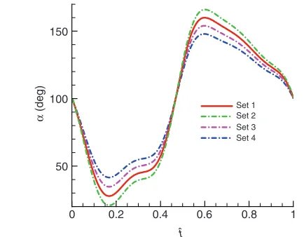
We make three additional sets of computations for hoverfly H3. Let the computations for H3 in the previous sections be known as set 1, in which the angle of attack at r2is the measured one. In the first additional set of computations, called set 2, the mid-downstroke

and mid-upstroke angles of attack at r2are decreased by about 10% from that of the measured . In the second and third additional sets of computations, called set 3 and set 4, respectively, the mid-downstroke and mid-upstroke angles of attack at r2are increased by about 10% and 20% from that of the measured , respectively. The time courses of angle of attack at r2in one cycle for these four sets are given in Fig.18. The computed mean force and power coefficients are given in Table4, and the computed power required for producing unit lift is given in Table5.

Several observations may be made concerning the data given in Tables 4 and 5. First, it is seen that the major results obtained above for the case of measured angle of attack are also obtained for the cases of higher and lower angles of attack. These results include:

CLand CDof the rigid flat-plate wing are about 10% and 4% smaller,

and CP,aabout 4% larger, than their counterparts of the deformable

wing; the aerodynamic power required for producing unit lift for the rigid flat-plate wing is about 15% higher than that of the deformable wing (for the wing with spanwise twist only and the wing with camber only, this number is about 10% and 6%, respectively). These results further strengthen the present analysis and remove any ambiguity regarding angle of attack changes that might be induced by removing camber and/or twist.

Second, it is seen (Table5) that when the angle of attack is increased, the power requirement per unit lift becomes higher. Using an angle of attack smaller (in set 2) than that used by the hovering hoverfly (in set 1, the measured one), the power required per unit lift can be reduced. It seems that the hovering hoverfly is not using the most energy-saving angle of attack to hover. But it should be noted that, if the angle of attack is decreased to that in set 2, the CL

would become 1.61, which is much smaller than that required to balance the weight (1.94).

LIST OF SYMBOLS AND ABBREVIATIONS

c mean chord length of the wing

Cd non-dimensional drag per unit wing length

CD coefficient of drag CD mean coefficient of drag

Cl non-dimensional lift per unit wing length

CL coefficient of lift CL mean coefficient of lift

CP,a coefficient of aerodynamic power CP,a mean coefficient of aerodynamic power LEV leading edge vortex

m mass of the insect

n wingbeat frequency

OXYZ an inertial frame, with the XYplane in the stroke plane and O at the wing root

p pressure

r radial position along the wing length

r2 radius of the second moment of wing area

R wing length

Re Reynolds number

Table 5. Aerodynamic power required for producing unit lift at various angles of attack at r2for hoverfly H3 (W N–1₎

I.D. A (deformable wing) B (flat-plate) C (twist only) D (camber only)

Set 1 4.04 4.64 4.44 4.27

Set 2 3.24 3.68 3.49 3.41

Set 3 4.61 5.28 5.02 4.83

Set 4 5.45 6.22 5.94 5.69

A, deformable wing; B, rigid flat-plate wing; C, wing with twist deformation only; D, wing with camber deformation only.

0 0.2 0.4 0.6 0.8 1

50 100 150

Set 1

Set 3 Set 2

Set 4

tˆ

α

(deg)

S wing area

t non-dimensional time u fluid velocity U reference speed

v kinematic viscosity

 local angle of attack of each wing section  deviation angle

 density

 stroke angle

 stroke amplitude  gradient operator 2 _{Laplacian operator}

ACKNOWLEDGEMENTS

This research was supported by a grant from the National Natural Science Foundation of China (10732030).

REFERENCES

Dickinson, M. H., Lehman, F. O. and Sane, S. P.(1999). Wing rotation and the aerodynamic basis of insect flight. Science284, 1954-1960.

Du, G. and Sun, M.(2008). Effects of unsteady deformation of flapping wings on its aerodynamic forces. Appl. Math. Mech.29, 731-741.

Ellington, C. P.(1984a). The aerodynamics of hovering insect flight. Morphological parameters. Philos. Trans. R. Soc. Lond. B. Biol. Sci.305, 1-15.

Ellington, C. P.(1984b). The aerodynamics of hovering insect flight. III. Kinematics. Philos. Trans. R. Soc. Lond. B. Biol. Sci.305, 41-78.

Ellington, C. P., Van Den Berg, C., Willmott, A. P. and Thomas, A. L. R. (1996). Leading-edge vortices in insect flight. Nature 384, 626-630.

Ennos, A. R.(1989). The kinematics and aerodynamics of the free flight of some Diptera. J. Exp. Biol.142, 49-85.

Liu, H., Ellington, C. P., Kawachi, K., Van Den Berg, C. and Willmott, A. P.(1998). A computational fluid dynamic study of hawkmoth hovering. J. Exp. Biol.201, 461-477.

Lu, Y., Shen, G. X. and Lai, G. J.(2006). Dual leading-edge vortexes on flapping wings.J. Exp. Biol.209, 5005-5016.

Morton, S. A., Melville, R. B. and Visbal, M. R.(1998). Accuracy and coupling issues of aeroelastic Navier-Stokes solutions on deforming meshes. J. Aircraft35, 798-805.

Rogers, S. E. and Kwak, D.(1990). Upwind differencing scheme for the time-accurate incompressible Navier-Stokes equations. AIAA J.28, 253-262.

Rogers, S. E., Kwak, D. and Kiris, C.(1991). Steady and unsteady solutions of the incompressible Navier-Stokes equations. AIAA J.29, 603-610.

Sane, S. P. and Dickinson, M. H.(2001). The control of flight force a flapping wing: lift and drag production. J. Exp. Biol.204, 2607-2626.

Sun, M. and Tang, J.(2002). Unsteady aerodynamic force generation by a model fruit fly wing in flapping motion. J. Exp. Biol.205, 55-70.

Sun, M. and Wu, J. H.(2004). Large aerodynamic force generation by a sweeping wing at low Reynolds numbers.Acta Mech. Sinica 20, 24-31.

Usherwood, J. R. and Ellington, C. P.(2002a). The aerodynamics of revolving wings. I. Model hawkmoth wings. J. Exp. Biol. 205, 1547-1564.

Usherwood, J. R. and Ellington, C. P.(2002b). The aerodynamics of revolving wings. II. Propeller force coefficients from mayfly to quail. J. Exp. Biol.205, 1565-1576.

Walker, S. M., Thomas, A. L. R. and Taylor, G. K.(2009). Deformable wing kinematics in free-flying hoverflies, J. R. Soc. Interface7, 131-142.

Wang, Z. J., Birch, J. M. and Dickinson, M. H.(2004). Unsteady forces and flows in flow Reynolds number hovering flight: two-dimensional computational vs robotic wing experiments. J. Exp. Biol.207, 269-283.

Wu, J. C.(1981). Theory for aerodynamic force and moment in viscous flows. AIAA J.

19, 432-441.

Wu, J. H. and Sun, M.(2004). Unsteady aerodynamic forces of a flapping wing. J. Exp. Biol.207, 1137-1150.

Young, J., Walker, S. M., Bomphrey, R. J., Taylor, G. K. and Thomas, L. R.(2009). Details of insect wing design and deformation enhance aerodynamic function and flight efficiency. Science, 325, 1549-1552.