Online Full Text

Abstract—A finite volume, cell-centered, density-based flow solver on unstructured grids is developed. The Weiss & Smith precondition matrix is implemented for solving flows of incompressible and variable density fluids at all speeds. The AUSMDV (Advection Upstream Splitting Method) scheme with a second order reconstruction is given for the explicit Runge-Kutta and implicit Lower-Upper Symmetric Gauss-Seidel (LU-SGS) time integration methods. Results are presented for inviscid flows through a channel with a bump at various Mach numbers, driven flows in a square cavity and inviscid/viscous flows in a planar supersonic nozzle. The performance of the flow solver with and without preconditioning is illustrated. General solution enhancement and convergence acceleration for steady-state Navier-Stokes solutions are attained via the use of inviscid/viscous preconditioning. The ability of the solver in providing accurate steady-state solutions for transonic and low-speed flow of variable density fluids is demonstrated.

Index Terms—Low speed preconditioning, flow solver, unstructured grids

I. INTRODUCTION

OMPUTATIONAL fluid dynamics (CFD) technologies are widely used in design and analysis process by industry, academia, and research community. The numerical flow solvers are challenged with demand to provide answers to more complex and wide ranging problems from incompressible to high-speed compressible flows. The incompressible flows were first addressed by pressure-based solution algorithms which are solved in an uncoupled manner. At the same time, density-based schemes were developed in the context of transonic and supersonic aerodynamic applications. These methods employ time-marching procedures that use the physical time derivatives, both implicit and explicit, to solve the hyperbolic system of governing equations.

A density-based flow solver is developed based on unstructured grids. The algorithms employed here are designed to compute steady-state flows of incompressible and variable density fluids at all speeds over a wide range of Mach numbers. The unstructured meshes are used to meet the demand of discretizing geometrically complex domains.

Manuscript received December 26, 2012.

Zheng Li is a Ph. D. candidate at School of Astronautics, Beijing University of Aeronautics and Astronautics (BUAA), Beijing, China. (phone: 86-010-82339476; e-mail: [email protected]).

Hongjun Xiang is a vice Professor at School of Astronautics, Beijing University of Aeronautics and Astronautics (BUAA), Beijing, China. (e-mail: [email protected]).

Traditional time-marching, density-based algorithms have been very successful in the computation of high-speed flows. However, at low Mach numbers, most of these solvers encounter degraded convergence speeds as the ratio of acoustic speeds to convective particle speeds increasing. Local preconditioning techniques have been first introduced to enable the simulation of an incompressible flow in a density-based flow solver. They remedy the ill-conditioned matrix equations by rescaling the eigenvalues of the governing equations. The goal of preconditioning methods is to reduce the disparity between the particle and acoustic wave speeds so that good convergence properties may be obtained at all speeds.

Three main development groups have appeared in the CFD literature for the preconditioning methods. The first group is Chorin [1] and Turkel [2], [3] who built a preconditioning method based on the artificial compressibility. The Turkel system is derived using entropy as the dependent variable. The second group including Choi, Merkle [4], Weiss, Smith [5], Venkateswaran, and Merkle [6] developed a family of preconditioners whose derivation is based on the temperature as the dependent variable. Lastly, the third group led by van Leer [7], developed a symmetric preconditioner which is referred as optimal since it equalizes the eigenvalues of the system for all Mach numbers.

In this paper we describe a finite volume, Navier-Stokes flow solver based on an unstructured grid topology that employs time-marching algorithm with Weiss-Smith preconditioning method. We will present the governing equations and the derivation of the preconditioning matrix for variable density flows, followed by a description of the spatial and temporal discretization. Finally, we present several results to demonstrate this methodology, including inviscid flows through a channel with a bump; driven flows in a square cavity and inviscid/viscous flows in a planar supersonic nozzle. These examples will provide a measure of the accuracy and performance of the present algorithm.

II. GOVERNING EQUATIONS

The fluid motion is governed by the time-dependent Navier-Stokes equations [5]. This system of equations, written to describe the mean flow properties, is cast in integral, Cartesian form for an arbitrary control volume V with differential surface area dA as follows:

∭ +∬[ − ]∙ = 0 (1) Where

The Development of a Navier-Stokes Flow

Solver with Preconditioning Method on

Unstructured Grids

Zheng Li, Hongjun Xiang

= ⎩ ⎪ ⎨ ⎪ ⎧ ⎭⎪⎬ ⎪ ⎫ , = ⎩ ⎪ ⎨ ⎪ ⎧ ₊ + + + ⎭⎪ ⎬ ⎪ ⎫ , = ⎩ ⎪ ⎨ ⎪ ⎧ 0 + ⎭⎪ ⎬ ⎪ ⎫

and , , , and are the density, velocity, total energy per unit mass, and pressure of the fluid, respectively. The term is the viscous stress tensor, is the heat flux vector, and

= + + is the position vector. For an idea gas, an equation of state, typically of the form = ( , ) where is the fluid temperature, must be specified along with (1) to describe the compressibility of the fluids.

III. PRECONDITIONING

A. Choice of Preconditioning Methods

In this section, comparisons have been made between the three low speed preconditioning methods introduced by Weiss-Smith, van Leer-Lee-Roe (VLR) and Turkle, respectively. The VLR preconditioner is better in convergence due to yielding the most optimal condition number (Fig. 1). In accuracy issues, all these preconditioners have the same impact. Although they are different in formula structure, they have a common point linked to the coefficient as the Mach number approach to zero. The most robust was found to be that proposed by Weiss and Smith which suffers only from the stagnation point singularity. Thus the Weiss–

Smith preconditioning method is implemented in our solver.

B. Weiss-Smith Precondition Matrix

According to [5], we transform the original system of equations from the conservative variables to the primitive variables = [ , , , , ] as follows:

∭ +∬[ − ]∙ = 0 (2) The original non preconditioned Jacobian ⁄ matrix can be replaced to a preconditioning matrix :

∭ +∬[ − ]∙ = 0 (3)

Γ=_⎜⎛

Θ 0 0 0

Θ 0 0

Θ 0 0

Θ 0 0

Θ −1 +

⎟ ⎞

Where Θ is given by

Θ= 1 −

Here is a reference velocity.

= | |, , | | << | | < , | | >

For the viscous low Reynolds number flows the reference velocity should not be smaller than the local diffusion velocity Δ ⁄ . Thus,

= max ( ,_Δ )

The resultant eigenvalues of the preconditioned system are given by

λ Γ

= , , , + , − ′

where

= (1− ) = + α= (1− ) 2⁄

β= ρ +

we can see that all eigenvalues remain of the order of u as long as the reference velocity is of the same order as the local velocity.

IV. SOLUTION PRECEDURE

A. Data Structure and Grid Entry

Contrary to structured solvers, the unstructured flow solver is much complex in data structure and grid entry due to its indirect data addressing. The procedure here is written in C++ with a set of classes to describe vertex, face, cell and their link. The solver can input the mesh generated by Gambit which is easier in partitioning grid over geometrically complex domains.

B. Spatial Discretization

The preconditioned governing equations are discretized spatially using a finite volume scheme wherein the physical domain is subdivided into small (nondeforming) hexahedron volumes and integral equations are applied to each cell. The discrete, inviscid flux vectors appearing in (1) are evaluated by AUSMDV (Advection Upstream Splitting Method) scheme with a modification to operate effectively at low Mach numbers. The schemes introduced by Liou have been discussed more thoroughly in [8] and [9].

C. Reconstruction

The solution vector Q used to evaluate the fluxes at cell faces is computed using a multidimensional linear reconstruction approach. In this approach, higher order accuracy is achieved at cell faces through a Taylor series expansion of the cell-averaged solution vector about the cell centroid:

= + ∙ (4) where is the displacement vector from the cell centroid to the face centroid. This formulation requires determining the solution gradient in each cell. This gradient is computed using the Green-Gauss theorem, which in discrete form is written as:

= ∑ (5) where is the volume of the cell, is the area of the face. The average solution vector is computed by adjacent cell, written as:

= ( + ) (6) Finally, the gradients are limited by the coefficient so that they do not introduce new maxima or minima into the reconstructed data. The Venkatakrishnan limiter [10] is implemented on this code.

D. Temporal Discretization

An explicit multistage time-stepping scheme and an implicit scheme are implemented on the preconditioned system using the conservative variables of unknowns. 1) Explicit Scheme

The explicit m-stage Runge-Kutta (R-K) scheme which solves the equation from time to time +∆ is given by

= (7) = − ∆ ( ) ₍₈₎ ∆ = ( ) (9) where = 1,2,3,… is the stage counter for the m-stage scheme and is the multistage coefficient for the th stage. 2) Implicit Scheme

The implicit Lower-Upper Symmetric Gauss-Seidel (LU-SGS) scheme for (1), see [11],can be described as: Forward sweep:

ΓΔ ∗_{= −0.5∑}

∙∆ ∗− : ∈ ( )

ΓΔ ∗ (10) Backward sweep:

ΓΔ =ΓΔ ∗_{−0.5 ∑}

∙∆ −

:∈ ()

ΓΔ (11) Res =−

() ∙ Where D is the diagonal matrix

D = _{∆t + 0.5} ()

V. RESULT

In this section, the preconditioning implementation for the unstructured flow solver has been assessed using some representative cases. The test cases chosen for this purpose include inviscid flow past a bump in a channel, laminar driven flow in square cavity and planar supersonic nozzle. The two dimensional test cases have been geometrically represented as three-dimensional cases by simply extending the geometry in the spanwise direction. The first result will show the performance of the present method for computing inviscid flows at various speeds. The second case will demonstrate the importance of preconditioning for solving low speed flows of variable density fluids. And in the final case we demonstrate the performance of the solver in transonic flows.

A. Inviscid Flow Past a Bump in a Channel

This test case validates the implementation of preconditioning for the inviscid flow over a 10% circular arc bump at various speeds. The symmetrical computation

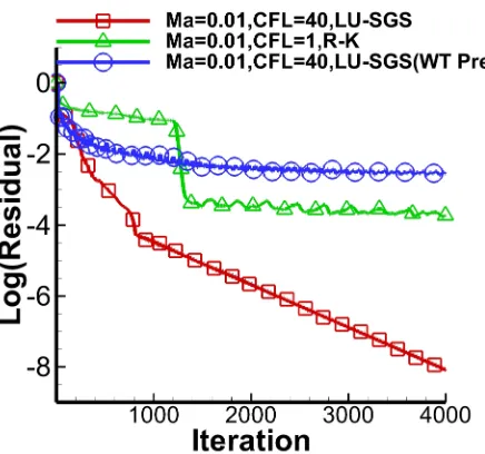
domain is 3×1 with a 129×65 grid partition. Fig. 2 shows the results in different methods at 0.01 Mach number over 4000 iteration cycles. Without preconditioning, the LU-SGS result is completely unphysical (Fig. 2a). The solution provided by R-K method with preconditioning (Fig. 2b) shows marked improvement but not well enough because of the limitation of CFL number. This drawback is corrected by using the LU-SGS implicit scheme (Fig. 2c). Fig. 3 provides an indication of the behavior of implementations of LU-SGS with preconditioning method for a range of Mach number. Fig. 4 and 5 highlights the convergence history in various conditions. Good efficiency across the Mach number range is obtained with the preconditioning method.

(a) LU-SGS, CFL=40, without preconditioning

(b) R-K, CFL=40, with preconditioning

(c) LU-SGS, CFL=40, with preconditioning Fig. 2 Density contour at Ma=0.01

(a) Ma=0.1 (b) Ma=0.2

B. Driven Flows in Square Cavity

This test case, representing a 2-dimensional laminar incompressible flow in a square cavity, has been numerical investigated in detail by Ghia [12] et al. The computation has been made with a uniform velocity at the top wall of the cavity. A set of Re numbers (100, 400, and 1000) are considered in this case. Fig. 6 and 7 shows the distribution of velocity through geometric center of the cavity. Fig. 8 gives the streamline pattern at 100 and 1000 Re number. The results show great agreement with the numerical simulations of Ghia. The convergence history is highlighted in Fig. 9. The ability in computation of laminar incompressible flow is demonstrated.

Fig. 4 Convergence histories for LU-SGS at various speeds

Fig. 5 Convergence histories with different time integration method

Fig. 6 -velocity along horizontal line through geometric center of cavity

Fig. 7 -velocity along vertical line through geometric center of cavity

C. Planar Supersonic Nozzle

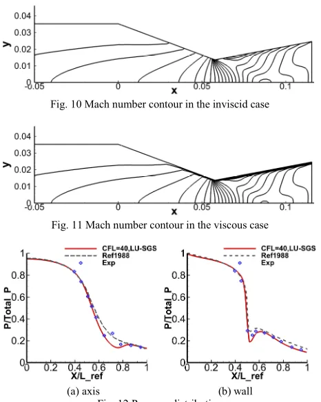
In this section, results are presented for a planar nozzle which is experimentally investigated by Mason et al [13]. This test case serves to validate the implementation of preconditioning at transonic flows. Both the (laminar) Navier- Stokes and Euler equations have been solved in the computation. No-slip condition was used at the wall for the Navier-Stokes equations. The inlet Mach number was taken as 0.232 and the ratio of the exit static pressure to the upstream stagnation pressure was fixed at 0.1135, corresponding to the design condition. The results solved by different equations are represented by Mach number in Fig. 10 and 11. Fig. 12 indicates the pressure distribution at wall and the axis. Comparisons with the experimental data and results in [14] show good agreement.

VI. CONCLUSION

In this paper, time-derivative low-speed preconditioning of the Navier-Stokes equations, suitable for both incompressible and compressible fluids has been successfully implemented on an unstructured flow solver. The AUSMDV scheme with a second order upwind-biased reconstruction is presented to accommodate the preconditioned eigenvalues and eigenvectors. Both explicit and implicit schemes are developed to march the solution of the preconditioned system to steady-state. To demonstrate the accuracy and efficiency of the present algorithm three test cases were presented. Substantial convergence enhancement and acceleration is shown at low Mach numbers when preconditioning is used with the inviscid solution. Convergence of the implicit scheme remains by far faster than the explicit scheme. General convergence enhancement is also demonstrated with the use of preconditioning on the Navier-Stokes equations at various speeds.

REFERENCES

[1] Chorin A. A numerical method for solving incompressible viscous flows problems [J]. J Comput Phys 1967:2:12-26.

[2] Turkel E. Preconditioning techniques in computational fluid dynamics [J]. Ann Rev Fluid Mech 1999:31:385-416.

[3] Turkel E, Radespiel R, Kroll N. Assessment of preconditioning methods for multidimensional aerodynamics [J]. Comput Fluids 1997:26:613-34.

[4] Choi Y, Merkle C. The application of preconditioning in viscous flows [J]. J Comput Phys 1993:105:207-23.

[5] Weiss J. Smith W. Preconditioning applied to variable and constant density flows [J]. AIAA J 1995:33:2050-6.

[6] Venkateswaran S. Merkle L. Analysis of preconditioning methods for the Euler and Navier-Stokes equations. Von Karman Institute for Fluid Dynamics, 1999.

[7] van Leer B, Lee W, Roe P. Characteristic time-stepping or local preconditioning of the Euler equations [J]. AIAA paper 91-1552:1991. [8] Liou, M.-S. Further Progress in Numerical Flux Scheme, Proceedings of the 15th International Confer-ence on Numerical Methods in Fluid Dynamics, June 1996.

[9] Edwards J, Liou M. Low-diffusion flux-splitting methods for flows at all speeds [J]. AIAA-97-1862.

[10] Venkatakrishnan V. On the accuracy of limiters and convergence to steady state solutions[C]. AIAA 93-0880.

[11] Sharov D, Nakahashi K. Low speed preconditioning and LU-SGS scheme for 3-D viscous flow computations on unstructured grids[C]. AIAA 98-0614.

[12] Ghia U. High-Re Solutions for Incompressible Flow Using the Navier-Stokes Equations and a Multigrid Method [J]. J Comput Phys，

1982:48:387-411.

[13] M. L. Mason, L. E. Putnam and R. J. Re, The Effect of Throat Contouring on Two-Dimensional Converging-Diverging Nozzles at Static Conditions, NASA Technical Paper 1704, 1980.

[14] Karki K, Patankar S. A Pressure Based Calculation Procedure for Viscous Flows at All Speeds in Arbitrary Configurations[C]. AIAA-88-0058.

Fig. 9 Convergence histories at different Re number

Fig. 10 Mach number contour in the inviscid case

Fig. 11 Mach number contour in the viscous case