Accurate Information Extraction from Research Papers using Conditional Random Fields

Accurate Information Extraction from Research Papers

using Conditional Random Fields

Fuchun Peng

Department of Computer Science

University of Massachusetts

Amherst, MA 01003

[email protected]

Andrew McCallum

Department of Computer Science

University of Massachusetts

Amherst, MA 01003

[email protected]

Abstract

With the increasing use of research paper search engines, such as CiteSeer, for both lit-erature search and hiring decisions, the accu-racy of such systems is of paramount impor-tance. This paper employs Conditional Ran-dom Fields (CRFs) for the task of extracting various common fields from the headers and citation of research papers. The basic the-ory of CRFs is becoming well-understood, but best-practices for applying them to real-world data requires additional exploration. This paper makes an empirical exploration of several fac-tors, including variations on Gaussian, expo-nential and hyperbolic-L1priors for improved

regularization, and several classes of features and Markov order. On a standard benchmark data set, we achieve new state-of-the-art perfor-mance, reducing error in average F1 by 36%, and word error rate by 78% in comparison with the previous best SVM results. Accuracy com-pares even more favorably against HMMs.

1

Introduction

Research paper search engines, such as CiteSeer (Lawrence et al., 1999) and Cora (McCallum et al., 2000), give researchers tremendous power and conve-nience in their research. They are also becoming increas-ingly used for recruiting and hiring decisions. Thus the information quality of such systems is of significant im-portance. This quality critically depends on an informa-tion extracinforma-tion component that extracts meta-data, such as title, author, institution, etc, from paper headers and references, because these meta-data are further used in many component applications such as field-based search, author analysis, and citation analysis.

Previous work in information extraction from research papers has been based on two major machine learn-ing techniques. The first is hidden Markov models (HMM) (Seymore et al., 1999; Takasu, 2003). An HMM learns a generative model over input sequence and labeled sequence pairs. While enjoying wide his-torical success, standard HMM models have difficulty modeling multiple non-independent features of the ob-servation sequence. The second technique is based on discriminatively-trained SVM classifiers (Han et al., 2003). These SVM classifiers can handle many non-independent features. However, for this sequence label-ing problem, Han et al. (2003) work in a two stages pro-cess: first classifying each line independently to assign it label, then adjusting these labels based on an additional classifier that examines larger windows of labels. Solving the information extraction problem in two steps looses the tight interaction between state transitions and obser-vations.

In this paper, we present results on this research paper meta-data extraction task using a Conditional Random Field (Lafferty et al., 2001), and explore several practi-cal issues in applying CRFs to information extraction in general. The CRF approach draws together the advan-tages of both finite state HMM and discriminative SVM techniques by allowing use of arbitrary, dependent fea-tures and joint inference over entire sequences.

CRFs have been previously applied to other tasks such as name entity extraction (McCallum and Li, 2003), table extraction (Pinto et al., 2003) and shallow parsing (Sha and Pereira, 2003). The basic theory of CRFs is now well-understood, but the best-practices for applying them to new, real-world data is still in an early-exploration phase. Here we explore two key practical issues: (1) reg-ularization, with an empirical study of Gaussian (Chen and Rosenfeld, 2000), exponential (Goodman, 2003), and hyperbolic-L1(Pinto et al., 2003) priors; (2) exploration

and layout, as well as proposing a method for the bene-ficial use of zero-count features without incurring large memory penalties.

We describe a large collection of experimental results on two traditional benchmark data sets. Dramatic im-provements are obtained in comparison with previous SVM and HMM based results.

2

Conditional Random Fields

Conditional random fields (CRFs) are undirected graph-ical models trained to maximize a conditional probabil-ity (Lafferty et al., 2001). A common special-case graph structure is a linear chain, which corresponds to a finite state machine, and is suitable for sequence labeling. A linear-chain CRF with parametersΛ = {λ, ...} defines a conditional probability for a state (or label1_{) sequence}

y=y1...yT given an input sequencex=x1...xT to be

Pλ(y|x) = 1

Zx exp

T

X

t=1

X

k

λkfk(yt−1, yt,x, t)

!

,

(1)

where Zx is the normalization constant that makes the probability of all state sequences sum to one, fk(yt−1, yt,x, t) is a feature function which is often

binary-valued, but can be real-valued, andλkis a learned

weight associated with featurefk. The feature functions

can measure any aspect of a state transition,yt−1 →yt,

and the observation sequence,x, centered at the current

time step, t. For example, one feature function might have value 1 whenyt−1is the state TITLE,ytis the state

AUTHOR, andxtis a word appearing in a lexicon of

peo-ple’s first names. Large positive values forλk indicate a

preference for such an event, while large negative values make the event unlikely.

Given such a model as defined in Equ. (1), the most probable labeling sequence for an inputx,

y∗= arg max

y PΛ(

y|x),

can be efficiently calculated by dynamic programming using the Viterbi algorithm. Calculating the marginal probability of states or transitions at each position in the sequence by a dynamic-programming-based infer-ence procedure very similar to forward-backward for hid-den Markov models.

The parameters may be estimated by maximum likelihood—maximizing the conditional probability of a set of label sequences, each given their correspond-ing input sequences. The log-likelihood of traincorrespond-ing set

1

We consider here only finite state models in which there is a one-to-one correspondence between states and labels; this is not, however, strictly necessary.

−6 −5 −4 −3 −2 −1 0 1 2 3 0

2 4 6 8 10 12

lambda

counts of lamda (in log scale)

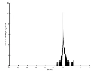
Figure 1: Empirical distribution ofλ

{(xi, yi) :i= 1, ...M}is written

LΛ=

X

i

logPΛ(yi|xi)

=X

i T

X

t=1

X

k

λkfk(yt−1, yt,x, t)−logZxi

!

.

(2)

Maximizing (2) corresponds to satisfying the follow-ing equality, wherein the the empirical count of each fea-ture matches its expected count according to the model PΛ(y|x).

X

i

fk(yt−1, yt, xi, t) =

X

i

PΛ(y|x)fk(yt−1, yt, xi, t)

CRFs share many of the advantageous properties of standard maximum entropy models, including their con-vex likelihood function, which guarantees that the learn-ing procedure converges to the global maximum. Tra-ditional maximum entropy learning algorithms, such as GIS and IIS (Pietra et al., 1995), can be used to train CRFs, however, it has been found that a quasi-Newton gradient-climber, BFGS, converges much faster (Malouf, 2002; Sha and Pereira, 2003). We use BFGS for opti-mization. In our experiments, we shall focus instead on two other aspects of CRF deployment, namely regulariza-tion and selecregulariza-tion of different model structure and feature types.

2.1 Regularization in CRFs

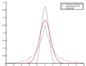
To avoid over-fitting, log-likelihood is often penalized by some prior distribution over the parameters. Figure 1 shows an empirical distribution of parameters,Λ, learned from an unpenalized likelihood, including only features with non-zero count in the training set. Three prior tributions that have shape similar to this empirical dis-tribution are the Gaussian prior, exponential prior, and hyperbolic-L1prior, each shown in Figure 2. In this

−100 −8 −6 −4 −2 0 2 4 6 8 10 0.05

0.1 0.15 0.2 0.25 0.3 0.35 0.4

Gaussian varianec=2 Exponential a=0.5 Hyperbolic

Figure 2: Shapes of prior distributions

2.1.1 Gaussian prior

With a Gaussian prior, log-likelihood (2) is penalized as follows:

LΛ=

X

i

logPΛ(yi|xi)−

X

k

λ2 k

2σ2 k

, (3)

whereσ2

kis a variance.

Maximizing (3) corresponds to satisfying

X

i

fk(yt−1, yt, xi, t)−

λk

σ2 k

=

X

i

PΛ(y|x)fk(yt−1, yt, xi, t)

This adjusted constraint (as well as the adjustments im-posed by the other two priors) is intuitively understand-able: rather than matching exact empirical feature fre-quencies, the model is tuned to match discounted feature frequencies. Chen and Rosenfeld (2000) discuss this in the context of other discounting procedures common in language modeling. We call the term subtracted from the empirical counts (in this caseλk/σ2) a discounted value.

The variance can be feature dependent. However for simplicity, constant variance is often used for all features. In this paper, however, we experiment with several alter-nate versions of Gaussian prior in which the variance is feature dependent.

Although Gaussian (and other) priors are gradually overcome by increasing amounts of training data, per-haps not at the right rate. The three methods below all provide ways to alter this rate by changing the variance of the Gaussian prior dependent on feature counts.

1. Threshold Cut: In language modeling, e.g, Good-Turing smoothing, only low frequency words are smoothed. Here we apply the same idea and only smooth those features whose frequencies are lower than a threshold (7 in our experiments, following standard practice in language modeling).

2. Divide Count: Here we let the discounted value for a feature depend on its frequency in the training

set,ck =P_iP_tfk(yt−1, yt,x, t). The discounted

value used here is λk

ck×σ2 whereσis a constant over all features. In this way, we increase the smoothing on the low frequency features more so than the high frequency features.

3. Bin-Based: We divide features into classes based on frequency. We bin features by frequency in the training set, and let the features in the same bin share the same variance. The discounted value is set to be

λk

dck/Ne×σ2 whereck is the count of features,N is the bin size, anddaeis the ceiling function. Alterna-tively, the variance in each bin may be set indepen-dently by cross-validation.

2.1.2 Exponential prior

Whereas the Gaussian prior penalizes according to the square of the weights (anL2penalizer), the intention here

is to create a smoothly differentiable analogue to penal-izing the absolute-value of the weights (anL1penalizer).

L1penalizers often result in more “sparse solutions,” in

which many features have weight nearly at zero, and thus provide a kind of soft feature selection that improves gen-eralization.

Goodman (2003) proposes an exponential prior, specifically a Laplacian prior, as an alternative to Gaus-sian prior. Under this prior,

LΛ=

X

i

logPΛ(yi|xi)−

X

k

αk|λk| (4)

whereαkis a parameter in exponential distribution.

Maximizing (4) would satisfy

X

i

fk(yt−1, yt, xi, t)−αk=

X

i

PΛ(y|x)fk(yt−1, yt, xi, t)

This corresponds to the absolute smoothing method in language modeling. We set theαk =α; i.e. all features

share the same constant whose value can be determined using absolute discountingα= n1

n1+2n2, wheren1andn2

are the number of features occurring once and twice (Ney et al., 1995).

2.1.3 Hyperbolic-L1prior

AnotherL1 penalizer is the hyperbolic-L1 prior,

de-scribed in (Pinto et al., 2003). The hyperbolic distribution has log-linear tails. Consequently the class of hyperbolic distribution is an important alternative to the class of nor-mal distributions and has been used for analyzing data from various scientific areas such as finance, though less frequently used in natural language processing.

Under a hyperbolic prior,

L_Λ=X

i

logP_Λ(yi|xi)−

X

k

log(e

λk_+e−λk

which corresponds to satisfying

X

i

fk(yt₋₁, yt, xi, t)−

e|λk|₋

e−|λk|

e|λk|+_e−|λk| =

X

i

PΛ(y|x)fi(yt₋₁, yt, xi, t)

The hyperbolic prior was also tested with CRFs in Mc-Callum and Li (2003).

2.2 Exploration of Feature Space

Wise choice of features is always vital the performance of any machine learning solution. Feature induction (Mc-Callum, 2003) has been shown to provide significant im-provements in CRFs performance. In some experiments described below we use feature induction. The focus in this section is on three other aspects of the feature space.

2.2.1 State transition features

In CRFs, state transitions are also represented as fea-tures. The feature functionfk(yt−1, yt,x, t)in Equ. (1)

is a general function over states and observations. Differ-ent state transition features can be defined to form dif-ferent Markov-order structures. We define four differ-ent state transitions features corresponding to differdiffer-ent Markov order for different classes of features. Higher order features model dependencies better, but also create more data sparse problem and require more memory in training.

1. First-order: Here the inputs are examined in the con-text of the current state only. The feature functions are represented asf(yt,x). There are no separate

parameters or preferences for state transitions at all.

2. First-order+transitions: Here we add parameters corresponding to state transitions. The feature func-tions used aref(yt,x), f(yt−1, yt).

3. Second-order: Here inputs are examined in the con-text of the current and previous states. Feature func-tion are represented asf(yt−1, yt,x).

4. Third-order: Here inputs are examined in the con-text of the current, two previous states. Feature func-tion are represented asf(yt−2, yt−1, yt,x).

2.2.2 Supported features and unsupported features

Before the use of prior distributions over parameters was common in maximum entropy classifiers, standard practice was to eliminate all features with zero count in the training data (the so-called unsupported features). However, unsupported, zero-count features can be ex-tremely useful for pushing Viterbi inference away from certain paths by assigning such features negative weight. The use of a prior allows the incorporation of unsup-ported features, however, doing so often greatly increases

the number parameters and thus the memory require-ments.

Below we experiment with models containing and not containing unsupported features—both with and without regularization by priors, and we argue that non-supported features are useful.

We present here incremental support, a method of in-troducing some useful unsupported features without ex-ploding the number of parameters with all unsupported features. The model is trained for several iterations with supported features only. Then inference determines the label sequences assigned high probability by the model. Incorrect transitions assigned high probability by the model are used to selectively add to the model those un-supported features that occur on those transitions, which may help improve performance by being assigned nega-tive weight in future training. If desired, several iterations of this procedure may be performed.

2.2.3 Local features, layout features and lexicon features

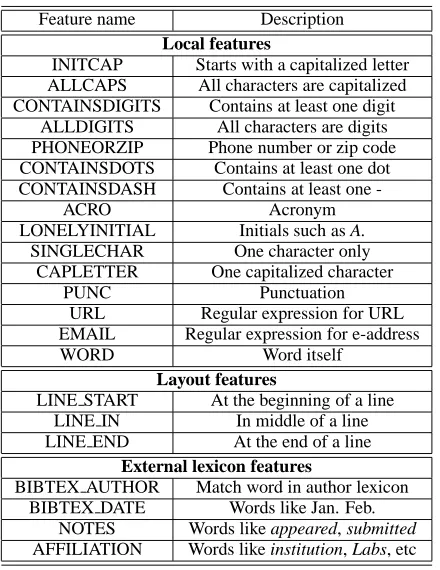
One of the advantages of CRFs and maximum entropy models in general is that they easily afford the use of arbi-trary features of the input. One can encode local spelling features, layout features such as positions of line breaks, as well as external lexicon features, all in one framework. We study all these features in our research paper extrac-tion problem, evaluate their individual contribuextrac-tions, and give some guidelines for selecting good features.

3

Empirical Study

3.1 Hidden Markov Models

Here we also briefly describe a HMM model we used in our experiments. We relax the independence assump-tion made in standard HMM and allow Markov depen-dencies among observations, e.g., P(ot|st, ot−1). We

can vary Markov orders in state transition and observa-tion transiobserva-tions. In our experiments, a model with second order state transitions and first order observation transi-tions performs the best. The state transition probabilities and emission probabilities are estimated using maximum likelihood estimation with absolute smoothing, which was found to be effective in previous experiments, includ-ing Seymore et al. (1999).

3.2 Datasets

3.2.1 Paper header dataset

The header of a research paper is defined to be all of the words from the beginning of the paper up to either the first section of the paper, usually the introduction, or to the end of the first page, whichever occurs first. It contains 15 fields to be extracted: title, author, affil-iation, address, note, email, date, abstract, introduction, phone, keywords, web, degree, publication number, and page (Seymore et al., 1999). The header dataset contains 935 headers. Following previous research (Seymore et al., 1999; McCallum et al., 2000; Han et al., 2003), for each trial we randomly select 500 for training and the re-maining 435 for testing. We refer this dataset as H.

3.2.2 Paper reference dataset

The reference dataset was created by the Cora project (McCallum et al., 2000). It contains 500 refer-ences, we use 350 for training and the rest 150 for test-ing. References contain 13 fields: author, title, editor, booktitle, date, journal, volume, tech, institution, pages, location, publisher, note. We refer this dataset as R.

3.3 Performance Measures

To give a comprehensive evaluation, we measure per-formance using several different metrics. In addition to the previously-usedword accuracymeasure (which over-emphasizes accuracy of the abstract field), we use per-field F1measure (both for individual fields and averaged over all fields—called a “macro average” in the informa-tion retrieval literature), andwhole instance accuracyfor measuring overall performance in a way that is sensitive to even a single error in any part of header or citation.

3.3.1 Measuring field-specific performance

1. Word Accuracy: We defineAas the number of true positive words, B as the number of false negative words,Cas the number of false positive words,D as the number of true negative words, andA+B+

C+Dis the total number of words. Word accuracy is calculated to be_A+B+C+DA+D

2. F1-measure: Precision, recall and F1 measure are defined as follows. Precision =_A+CA Recall =_A+BA F1 =2×_{P recision+Recall}P recision×Recall

3.3.2 Measuring overall performance

1. Overall word accuracy: Overall word accuracy is the percentage of words whose predicted labels equal their true labels. Word accuracy favors fields with large number of words, such as the abstract.

2. Averaged F-measure: Averaged F-measure is com-puted by averaging the F1-measures over all fields. Average F-measure favors labels with small num-ber of words, which complements word accuracy.

Thus, we consider both word accuracy and average F-measure in evaluation.

3. Whole instance accuracy: An instance here is de-fined to be a single header or reference. Whole instance accuracy is the percentage of instances in which every word is correctly labeled.

3.4 Experimental Results

We first report the overall results by comparing CRFs with HMMs, and with the previously best benchmark re-sults obtained by SVMs (Han et al., 2003). We then break down the results to analyze various factors individually. Table 1 shows the results on dataset H with the best re-sults in bold; (intro and page fields are not shown, fol-lowing past practice (Seymore et al., 1999; Han et al., 2003)). The results we obtained with CRFs use second-order state transition features, layout features, as well as supported and unsupported features. Feature induction is used in experiments on dataset R; (it didn’t improve accuracy on H). The results we obtained with the HMM model use a second order model for transitions, and a first order for observations. The results on SVM is obtained from (Han et al., 2003) by computing F1 measures from the precision and recall numbers they report.

HMM CRF SVM

Overall acc. 93.1% 98.3% 92.9% Instance acc. 4.13% 73.3%

-acc. F1 acc. F1 acc. F1 Title 98.2 82.2 99.7 97.1 98.9 96.5 Author 98.7 81.0 99.8 97.5 99.3 97.2 Affiliation 98.3 85.1 99.7 97.0 98.1 93.8 Address 99.1 84.8 99.7 95.8 99.1 94.7 Note 97.8 81.4 98.8 91.2 95.5 81.6 Email 99.9 92.5 99.9 95.3 99.6 91.7 Date 99.8 80.6 99.9 95.0 99.7 90.2 Abstract 97.1 98.0 99.6 99.7 97.5 93.8 Phone 99.8 53.8 99.9 97.9 99.9 92.4 Keyword 98.7 40.6 99.7 88.8 99.2 88.5 Web 99.9 68.6 99.9 94.1 99.9 92.4 Degree 99.5 68.8 99.8 84.9 99.5 70.1 Pubnum 99.8 64.2 99.9 86.6 99.9 89.2 Average F1 75.6 93.9 89.7

Table 1: Extraction results for paper headers on H

Table 2 shows the results on dataset R. SVM results are not available for these datasets.

3.5 Analysis

3.5.1 Overall performance comparison

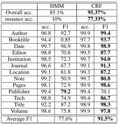
HMM CRF Overall acc. 85.1% 95.37% instance acc. 10% 77.33% acc. F1 acc. F1 Author 96.8 92.7 99.9 99.4 Booktitle 94.4 0.85 97.7 93.7 Date 99.7 96.9 99.8 98.9 Editor 98.8 70.8 99.5 87.7 Institution 98.5 72.3 99.7 94.0 Journal 96.6 67.7 99.1 91.3 Location 99.1 81.8 99.3 87.2 Note 99.2 50.9 99.7 80.8 Pages 98.1 72.9 99.9 98.6 Publisher 99.4 79.2 99.4 76.1 Tech 98.8 74.9 99.4 86.7 Title 92.2 87.2 98.9 98.3 Volume 98.6 75.8 99.9 97.8 Average F1 77.6% 91.5%

Table 2: Extraction results for paper references on R

2003). CRFs also perform significantly better than SVM-based approach, yielding new state of the art performance on this task. CRFs increase the performance on nearly all the fields. The overall word accuracy is improved from 92.9% to 98.3%, which corresponds to a 78% error rate reduction. However, as we can see word accuracy can be misleading since HMM model even has a higher word ac-curacy than SVM, although it performs much worse than SVM in most individual fields except abstract. Interest-ingly, HMM performs much better on abstract field (98% versus 93.8% F-measure) which pushes the overall accu-racy up. A better comparison can be made by compar-ing the field-based F-measures. Here, in comparison to the SVM, CRFs improve the F1 measure from 89.7% to 93.9%, an error reduction of 36%.

3.5.2 Effects of regularization

The results of different regularization methods are summarized in Table (3). Setting Gaussian variance of features depending on feature count performs better, from 90.5% to 91.2%, an error reduction of 7%, when only using supported features, and an error reduction of 9% when using supported and unsupported features. Re-sults are averaged over 5 random runs, with an aver-age variance of 0.2%. In our experiments we found the Gaussian prior to consistently perform better than the others. Surprisingly, exponential prior hurts the perfor-mance significantly. It over penalizes the likelihood (sig-nificantly increasing cost—defined as negative penalized log-likelihood). We hypothesized that the problem could be that the choice of constantαis inappropriate. So we tried varying α instead of computing it using absolute discounting, but found the alternatives to perform worse. These results suggest that Gaussian prior is a safer prior

support feat. all features

Method F1 F1

Gaussian infinity 90.5 93.3 Gaussian variance = 0.1 81.7 91.8 Gaussian variance = 0.5 87.2 93.0 Gaussian variance = 5 90.1 93.7 Gaussian variance = 10 89.9 93.5 Gaussian cut 7 90.1 93.4 Gaussian divide count 90.9 92.8 Gaussian bin 5 90.9 93.6 Gaussian bin 10 90.2 92.9 Gaussian bin 15 91.2 93.9 Gaussian bin 20 90.4 93.2 Hyperbolic 89.4 92.8 Exponential 80.5 85.6

Table 3: Regularization comparisons: Gaussian infinity is non-regularized, Gaussian variance = X sets variance to be X. Gaussian cut 7 refers to the Threshold Cut method,

Gaussian divide count refers to the Divide Count method, Gaussian bin N refers to the Bin-Based method with bin

size equals N, as described in 2.1.1

to use in practice.

3.5.3 Effects of exploring feature space

State transition features and unsupported features.

We summarize the comparison of different state tran-sition models using or not using unsupported features in Table 4. The first column describes the four different state transition models, the second column contains the overall word accuracy of these models using only support fea-tures, and the third column contains the result of using all features, including unsupported features. Comparing the rows, one can see that the second-order model per-forms the best, but not dramatically better than the first-order+transitions and the third order model. However, the first-order model performs significantly worse. The dif-ference does not come from sharing the weights, but from ignoring thef(yt−1, yt). The first order transition feature

is vital here. We would expect the third order model to perform better if enough training data were available.

Comparing the second and the third columns, we can see that using all features including unsupported features, consistently performs better than ignoring them. Our preliminary experiments with incremental support have shown performance in between that of supported-only and all features, and are still ongoing.

Effects of layout features

support all first-order 89.0 90.4 first-order+trans 95.6

-second-order 96.0 96.5 third-order 95.3 96.1

Table 4: Effects of using unsupported features and state transitions on H

Feature name Description Local features

INITCAP Starts with a capitalized letter ALLCAPS All characters are capitalized CONTAINSDIGITS Contains at least one digit

ALLDIGITS All characters are digits PHONEORZIP Phone number or zip code CONTAINSDOTS Contains at least one dot CONTAINSDASH Contains at least one

-ACRO Acronym

LONELYINITIAL Initials such as A. SINGLECHAR One character only

CAPLETTER One capitalized character PUNC Punctuation

URL Regular expression for URL EMAIL Regular expression for e-address WORD Word itself

Layout features

LINE START At the beginning of a line LINE IN In middle of a line LINE END At the end of a line

External lexicon features

BIBTEX AUTHOR Match word in author lexicon BIBTEX DATE Words like Jan. Feb.

NOTES Words like appeared, submitted AFFILIATION Words like institution, Labs, etc

Table 5: List of features used

The results of using different features are shown in Ta-ble 6. The layout feature dramatically increases the per-formance, raising the F1 measure from 88.8% to 93.9%, whole sentence accuracy from 40.1% to 72.4%. Adding lexicon features alone improves the performance. How-ever, when combing lexicon features and layout fea-tures, the performance is worse than using layout features alone.

The lexicons were gathered from a large collection of BibTeX files, and upon examination had difficult to re-move noise, for example words in the author lexicon that were also affiliations. In previous work, we have gained significant benefits by dividing each lexicon into sections based on point-wise information gain with respect to the lexicon’s class.

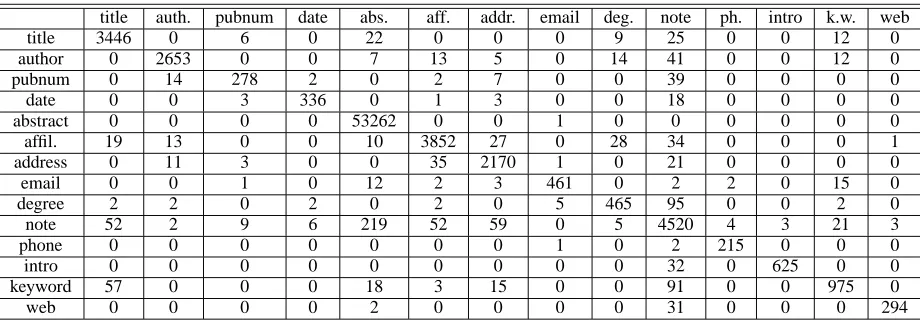
3.5.4 Error analysis

Table 7 is the classification confusion matrix of header extraction (field page is not shown to save space). Most

Word Acc. F1 Inst. Acc. local feature 96.5% 88.8% 40.1%

+ lexicon 96.9% 89.9% 53.1% + layout feature 98.2% 93.4% 72.4% + layout + lexicon 98.0% 93.0% 71.7%

Table 6: Results of using different features on H

errors happen at the boundaries between two fields. Es-pecially the transition from author to affiliation, from

ab-stract to keyword. The note field is the one most

con-fused with others, and upon inspection is actually labeled inconsistently in the training data. Other errors could be fixed with additional feature engineering—for exam-ple, including additional specialized regular expressions should make email accuracy nearly perfect. Increasing the amount of training data would also be expected to help significantly, as indicated by consistent nearly per-fect accuracy on the training set.

4

Conclusions and Future Work

This paper investigates the issues of regularization, fea-ture spaces, and efficient use of unsupported feafea-tures in CRFs, with an application to information extraction from research papers.

For regularization we find that the Gaussian prior with variance depending on feature frequencies performs bet-ter than several other albet-ternatives in the libet-terature. Feature engineering is a key component of any machine learn-ing solution—especially in conditionally-trained mod-els with such freedom to choose arbitrary features—and plays an even more important role than regularization.

We obtain new state-of-the-art performance in extract-ing standard fields from research papers, with a signifi-cant error reduction by several metrics. We also suggest better evaluation metrics to facilitate future research in this task—especially field-F1, rather than word accuracy. We have provided an empirical exploration of a few previously-published priors for conditionally-trained log-linear models. Fundamental advances in regularization for CRFs remains a significant open research area.

5

Acknowledgments

rec-title auth. pubnum date abs. aff. addr. email deg. note ph. intro k.w. web

title 3446 0 6 0 22 0 0 0 9 25 0 0 12 0

author 0 2653 0 0 7 13 5 0 14 41 0 0 12 0

pubnum 0 14 278 2 0 2 7 0 0 39 0 0 0 0

date 0 0 3 336 0 1 3 0 0 18 0 0 0 0

abstract 0 0 0 0 53262 0 0 1 0 0 0 0 0 0

affil. 19 13 0 0 10 3852 27 0 28 34 0 0 0 1

address 0 11 3 0 0 35 2170 1 0 21 0 0 0 0

email 0 0 1 0 12 2 3 461 0 2 2 0 15 0

degree 2 2 0 2 0 2 0 5 465 95 0 0 2 0

note 52 2 9 6 219 52 59 0 5 4520 4 3 21 3

phone 0 0 0 0 0 0 0 1 0 2 215 0 0 0

intro 0 0 0 0 0 0 0 0 0 32 0 625 0 0

keyword 57 0 0 0 18 3 15 0 0 91 0 0 975 0

web 0 0 0 0 2 0 0 0 0 31 0 0 0 294

Table 7: Confusion matrix on H

ommendations expressed in this material are the author(s) and do not necessarily reflect those of the sponsor.

References

S. Chen and R. Rosenfeld. 2000. A Survey of Smoothing Techniques for ME Models. IEEE Trans. Speech and

Audio Processing, 8(1), pp. 37–50. January 2000.

J. Goodman. 2003. Exponential Priors for Maximum Entropy Models. MSR Technical report, 2003.

H. Han, C. Giles, E. Manavoglu, H. Zha, Z. Zhang, and E. Fox. 2003. Automatic Document Meta-data Extrac-tion using Support Vector Machines. In Proceedings

of Joint Conference on Digital Libraries 2003.

J. Lafferty, A. McCallum and F. Pereira. 2001. Condi-tional Random Fields: Probabilistic Models for Seg-menting and Labeling Sequence Data. In

Proceed-ings of International Conference on Machine Learning 2001.

S. Lawrence, C. L. Giles, and K. Bollacker. 1999. Digital Libraries and Autonomous Citation Indexing. IEEE

Computer, 32(6): 67-71.

R. Malouf. 2002. A Comparison of Algorithms for Max-imum Entropy Parameter Estimation. In Proceedings

of the Sixth Conference on Natural Language Learning (CoNLL)

A. McCallum. 2003. Efficiently Inducing Features of Conditional Random Fields. In Proceedings of

Conference on Uncertainty in Articifical Intelligence (UAI).

A. McCallum, K. Nigam, J. Rennie, K. Seymore. 2000. Automating the Construction of Internet Portals with Machine Learning. Information Retrieval Journal,

volume 3, pages 127-163. Kluwer. 2000.

A. McCallum and W. Li. 2003. Early Results for Named Entity Recognition with Conditional Random Fields, Feature Induction and Web-Enhanced Lexicons. In

Proceedings of Seventh Conference on Natural Lan-guage Learning (CoNLL).

H. Ney, U. Essen, and R. Kneser 1995. On the Estima-tion of Small Probabilities by Leaving-One-Out. IEEE

Transactions on Pattern Analysis and Machine Intelli-gence, 17(12):1202-1212, 1995.

S. Pietra, V. Pietra, J. Lafferty 1995. Inducing Fea-tures Of Random Fields. IEEE Transactions on

Pat-tern Analysis and Machine Intelligence, Vol. 19, No.

4.

D. Pinto, A. McCallum, X. Wei and W. Croft. 2003. Ta-ble Extraction Using Conditional Random Fields. In

Proceedins of the 26th Annual International ACM SI-GIR Conference on Research and Development in In-formation Retrieval (SIGIR’03)

K. Seymore, A. McCallum, R. Rosenfeld. 1999. Learn-ing Hidden Markov Model Structure for Information Extraction. In Proceedings of AAAI’99 Workshop on

Machine Learning for Information Extraction.

F. Sha and F. Pereira. 2003. Shallow Parsing with Con-ditional Random Fields. In Proceedings of Human

Language Technology Conference and North Ameri-can Chapter of the Association for Computational Lin-guistics (HLT-NAACL’03)

A. Takasu. 2003. Bibliographic Attribute Extrac-tion from Erroneous References Based on a Statistical Model. In Proceedings of Joint Conference on Digital