Use of nonparametric regression methods for developing a local stem form model

Use of nonparametric regression methods for developing

a local stem form model

K. Kuželka, R. Marušák

Faculty of Forestry and Wood Sciences, Czech University of Life Sciences Prague, Prague, Czech Republic

ABSTRACT:A local mean stem curve of spruce was represented using regression splines. Abilities of smoothing spline and P-spline to model the mean stem curve were evaluated using data of 85 carefully measured stems of Norway spruce. For both techniques the optimal amount of smoothing was investigated in dependence on the number of training stems using a cross-validation method. Representatives of main groups of parametric models – single models, segmented models and models with variable coefficient – were compared with spline models using five statistic criteria. Both regression splines performed comparably or better as all representatives of parametric models independently of the numbers of stems used as training data.

Keywords: Norway spruce, spline; stem curve; taper

JOURNAL OF FOREST SCIENCE, 60, 2014 (11): 464–471

The extensive development of taper models and stem form equations during the last decades report-ed in scientific literature has evidencreport-ed a continual interest in this beneficial tool of forest manage-ment. Stem form models expressed as a functional dependence of stem diameter at a given height on this height (Sharma, Parton 2009) allow to assess stem diameter at any height. Consequently, the vol-ume of any specified log can be calculated and the assortment structure estimated (Rojo et al. 2005).

The stem form is a result of many factors (Mu-hairwe et al. 1994) including genetic influences (Gomat et al. 2011), stand density (Sharma, Par-ton 2009), thinning (Sharma et al. 2002), pruning (Valenti, Cao 1986), water availability (Wiklund et al. 1995) and supply of other resources. A huge number of the factors are stand specific; they influ-ence almost all trees in a stand in the same way. Stem curves in a stand – or more generalized in a locality – tend to have the identical shape and therefore they can be described by a local stem curve model.

Mixed-effect models (Lejeune et al. 2009; Cao, Wang 2011) were developed in the last years in

order to match individual stems to a general stem curve using one or more upper stem diameters. As-suming a similar stem curve for trees in a locality a population-specific model can be derived as the mean stem curve. The local model can be matched to height and diameter at breast height of an indi-vidual tree. A number of such models was devel-oped: simple models of polynomial (Bruce et al. 1968; Kozak et al. 1969), logarithmic (Demaer-schalk 1972), trigonometric (Thomas, Par-resol 1991), sigmoidal (Biging 1984) and other forms, segmented models (Max, Burkhart 1976; Brooks et al. 2008) and various models with vari-able exponent (Newberry, Burkhart 1986; Lee et al. 2003). Most of recent works (Rojo et al. 2005; Li, Weiskittel 2010) comparing taper models re-port the variable-form models to have a superior performance than the single or segmented models due to their flexibility.

Non-parametric and spline models are even more flexible. Splines were used to interpolate an indi-vidual stem curve from a set of measured diameters (Figueiredo-Filho et al. 1996; Laasasenaho et al. 2005). Non-parametric and spline regression

techniques serve also as a regression model of the mean stem curve. Smoothing spline was used to fit the stem curve represented as a set of average di-ameters at relative heights (Lappi 2006; Kublin et al. 2008) or to predict the stem curve if a part of the stem curve was known (Nummi, Mottonen 2004; Koskela et al. 2006). Kublin et al. (2013) used B-spline to develop a general stem curve model adaptable to an individual stem.

The objective of this study is to explore possi-bilities of using two types of regression splines to develop a model of local mean stem curve. Spline models are compared to commonly used paramet-ric models.

MATERIAL AND METHODS

Data. This study used data from 85 Norway spruce sample trees (Picea abies [L.] Karst.). The trees were from three even-aged pure plantations with ages from 50 to 100 years located in the School Forest En-terprise Kostelec nad Černými lesy, Czech Republic. The diameter at breast height (DBH) ranged from 88 to 438 mm (mean 204 mm), and tree heights ranged from 10.6 to 37.1 m (mean 21.3 m). Trees were felled and subsequently diameters outside bark were measured from the tree base to the top at 0.1-m intervals. The distances from the tree base were measured using a steel tape with 0.01-m precision, and the diameters were measured and recorded with an electronic calliper with 1-mm precision.

Spline regression models and parameter op-timization. Two regression splines were used to model the mean stem curve: smoothing spline and P-spline. Smoothing spline (SS) is a twice continu-ous curve that relates the requirement of minimal curvature with the requirement of the minimal re-sidual sum of squares. The importance of minimi-zation of the residual sum of squares is expressed as smoothing parameter λ (Aydin 2007). P-spline (PS) is a penalized spline regression estimator based on B-spline with a flexible number of knots. To restrict the roughness of the curve kth_-order

dif-ference penalty is used (Eilers, Marx 1996). Ex-cept the smoothing parameter λ also the number of knots is important. Too many knots lead to overfit-ting and too few knots lead to underfitoverfit-ting.

Both spline models were fitted using the nor-malized height-diameter data. For both methods the optimal amount of smoothing must be deter-mined. This was carried out using the leave-one-out cross-validation (LOOCV) approach; the best λ is the value that minimizes LOOCV value. For

smoothing spline λ can take any value from the close range from 0 to1; λ = 0 leads to a regression line, λ = 1 leads to spline interpolation. The behav-iour of SS was examined with 20 values of λ: 10–6_,

10–5_{, …, 10}–1_{, 0.2, 0.4, 0.6, 0.8, 1–10}–1_{, 1–10}–2_{, … ,}

1–10–10_{. The amount of smoothing was optimized}

for different numbers of input points expressed in two ways. Firstly, λ was optimized for 1 to 50 stems with measured diameters with inter-spaces of 2 m (15 to 845 data points). Secondly, λ was optimized for different densities of data points expressed by interspace lengths between measured diameters ‒ for several numbers of stem profiles the interspaces between diameters were set to 0.1, 0.2, 0.3, 0.4 and 0.5 m. For P-spline λ can take any non-negative number; with λ = 0, PS becomes a polynomial fit; as λ approaches in-finity, PS becomes a linear regression function. The set of λ values for describing the behaviour of PS smoothing consists of powers of two with exponents from –10 to 12. Also the influence of different numbers of knots must be considered. Powers of two with exponents from 1 to 9 were used as the number of knots.

Comparison of taper models. The performance of spline models is compared with parametric models. Based on comparison by Rojo et al. (2005) the fol-lowing models are selected for the comparison. The model of Cervera (Rojo et al. 2005) and the model of Max and Burkhart (1976) were selected as the best representatives of polynomial and segmented models, respectively. Because the variable exponent models are designated as the most accurate models, two of them were selected for the comparison; the model of Bi (2000), which is considered as the best in model comparison, and the model proposed by Lee et al. (2003). For fitting the models 85 spruce stem pro-files with 2 m long interspaces were employed.

The parametric models were fitted using the least-squares method. For fitting the non-linear functions of variable-exponent taper models, the Levenberg-Marquardt algorithm was used. The comparison of models was carried out using the LOOCV approach. A single stem is retained as validation data, while all other stems are used as training data to compute a regression spline or to fit a taper model. Residuals are assessed for each position of measured diam-eters of the validation stem. The residual values of each validation stem are evaluated using the criteria listed in Table 1. This procedure is repeated for all stems, so that every single stem serves as validation data exactly once.

stems were selected randomly from the whole data set. From the remaining stems, one was randomly selected for validation. The procedure was repeated 400 times in order to increase the accuracy of criteria estimation.

Because the variances of the criteria were not equal in all cases, the Kruskal-Wallis test with Tukey’s hon-estly significant difference test comparing average group ranks were used to test the equality of mean values of the criteria among taper models. Friedman’s test was used to determine the effect of the number of data points. To find if the means of diameter bias and total volume difference are different from zero one-sample t-test was used.

RESULTS

Optimal amount of smoothing

The development of cross-validation (CV) criterion in dependence on λ for smoothing spline is shown in Fig. 1. The development is very similar for all point densities. The minimum CV is found with λ between 1–10–4 _{and 1–10}–6 _{in dependence on point density.}

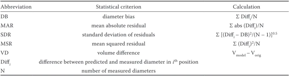
Table 1. Statistical criteria used for evaluating the accuracy of the models

Abbreviation Statistical criterion Calculation

DB diameter bias Σ Diff_i/N

MAR mean absolute residual Σ abs (Diff_i)/N

SDR standard deviation of residuals Σ [(Diff_i– DB)2_{/(N – 1)]}0.5

MSR mean squared residual Σ (Diff_i)2_/N

VD volume difference V_model –V_orig

Diff_i difference between predicted and measured diameter in ith _position

N number of measured diameters

abs – absolute value, V_model – stem volume based on stem curve model,V_orig – stem volume based on original measured stem profile

Fig. 1. Cross-validation values in dependence on smoothing param-eter for smoothing spline. Sepa-rate lines show the development of CV criterion for different density of training points expressed as the number of trees

However, within the range the change of CV is negli-gible. Outside that range the value of CV steeply in-creases. This tendency is observable in all input point densities. The same results are obtained in the case of expressing the point density in terms of the length of input point interspaces. Because the development of CV criterion in dependence on λ value was observed in several discrete points only, it can be concluded that the optimal amount of smoothing is achieved with λ ranging between 1–10–4 _{and 1–10}–6_.

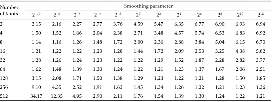
It is obvious that the development of CV crite-rion with changing λ in P-splines is strongly depen-dent on the number of segments (Table 2). With low numbers of segments the optimal values of λ, having the lowest values of CV criterion, are also low. For the rising number of knots, the optimal λ also increases. A regression analysis was carried out describing the dependence of the optimal λ on the number of knots. The λ values with the low-est CV criterion are plotted against their respec-tive number-of-knots. A regression power function (λ = β₁ × n_knots) fits nearly exactly all the data points (β₁ = 1.526 × 10–5_{, β}

2 = 3; R2 = 1.00). For a given

num-ber of knots the optimal value of λ is stable for differ-ent numbers of input points.

Comparison with selected parametric models

With rising numbers of stems the values of absolute diameter errors as well as absolute volume differences decline. The decline of the error values both for di-ameters and volume proved significant. The depen-dence of accuracy on the number of stems differed for different models. For the model of Bi (2000) the accuracy drop with lower number of stems was very pronounced. While with 84 training stems its accu-racy was very good in comparison with other models, for five stems the performance of the model was very poor. On the other hand, the model of Lee had the lowest accuracy among all models with a high num-ber of stems used, while for a low numnum-ber of stems the accuracy of its predictions was comparable with the other models.

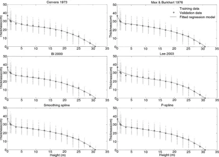
With 84 stems used to derive the model (Table 3, Fig. 2), both splines represented the mean function of typical stem curve very well. There was no system-atic error in diameter prediction nor in volume esti-mation. The mean errors for both diameter (less than

2 mm) and volume (less than 1%) prediction were very low. However, the mean absolute residuals as-sume quite high values, and also the variances of DB and TVD are high, which corresponds with the high values of mean absolute volume differences.

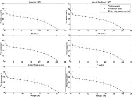
With lowering the number of stems (Table 4, Fig. 3), the diameter predictions of all models became sig-nificantly biased. With only five stems used to pa-rameterize the model no significant diameter bias was found with the model of Bi, which is caused by high variance of the prediction errors.

Concerning the criteria expressing the quality of fit of the curve (MAR, SDR, MSR) two groups of models with significantly different accuracy can be distinguished. For a high number of stems used for model parameterization the segmented polynomial model of Max and Burkhart (1976), the variable-exponent model of Bi (2000), and both spline models show better results than the single polynomial model of Cervera and the variable-exponent model of Lee et al. (2003). With a lower number of trees the most ac-curate models are the segmented polynomial model

Table 2. Cross-validation values in dependence on smoothing parameter and number of knots

Number of knots

Smoothing parameter

2–10 ₂–8 ₂–6 ₂–4 ₂–2 ₂0 ₂2 ₂4 ₂6 ₂8 ₂10 ₂12

2 2.15 2.16 2.27 2.77 3.76 4.59 5.47 6.35 6.77 6.90 6.93 6.94

4 1.50 1.52 1.66 2.04 2.38 2.71 3.48 4.57 5.74 6.53 6.83 6.92

8 1.14 1.16 1.26 1.48 1.72 2.00 2.36 2.88 3.84 5.04 6.15 6.70

16 1.21 1.22 1.22 1.23 1.28 1.44 1.72 2.09 2.53 3.25 4.38 5.62

32 1.28 1.26 1.24 1.23 1.22 1.22 1.29 1.52 1.87 2.28 2.82 3.77

64 1.62 1.48 1.39 1.30 1.24 1.22 1.21 1.23 1.37 1.67 2.06 2.51

128 3.15 2.08 1.71 1.50 1.38 1.29 1.23 1.22 1.21 1.28 1.50 1.85

256 9.10 4.35 2.52 1.91 1.63 1.45 1.34 1.26 1.22 1.21 1.23 1.36

512 34.17 12.35 4.95 2.90 2.11 1.76 1.54 1.39 1.30 1.24 1.22 1.21

Table 3. Comparison of taper models based on 84 stems

Model DB (10–2 m) MAR (10–2 m) SDR (10–2 m) MSR (10–3 m2) TVD (%) mean ± SD

Cervera 0.26 ± 1.27a _{1.58 ± 0.60}a _{1.88 ± 0.56}a _{0.44 ± 0.33}a _{–1.22 ± 6.61}a

Max-Bur-khart 0.18 ± 1.31a 1.32 ± 0.68b 1.52 ± 0.67b 0.34 ± 0.35b –0.24 ± 6.73a Bi 0.01 ± 1.09a _{1.31 ± 0.60}b _{1.55 ± 0.62}b _{0.32 ± 0.27}b _{–0.95 ± 5.69}a Lee 0.22 ± 1.10a _{1.56 ± 0.50}a _{1.93 ± 0.48}a _{0.43 ± 0.25}a _{0.09 ± 5.70}a Smoothing

spline 0.19 ± 1.34a 1.37 ± 0.68a,b 1.56 ± 0.65b 0.35 ± 0.34b 0.59 ± 6.75a P-spline 0.13 ± 1.31a _{1.31 ± 0.67}b _{1.50 ± 0.66}b _{0.33 ± 0.34}b _{–0.29 ± 6.69}a

together with the PS model; lower accuracy was ob-served with the SS models. The single polynomial model and both variable-exponent models showed significantly higher errors.

DISCUSSION

It was stated many times (Max 1976; Max, Bur-khart 1976; Jiang et al. 2005) that the single poly-nomial models are too rigid to conform to the

compli-cated shape of stem curve. This fact proved true also in this comparison, where the model considered as the best among the single polynomial models (Rojo et al. 2005) was outperformed by other models.

The rather complicated variable-exponent model of Bi (2000) is able to produce accurate predictions if the model parameter values are derived from a high number of stem profiles. In the comparison of Rojo et al. (2005) the models were parameterized using stem profiles of 203 stems. From this study it results that the model must be parameterized using at least

Table 4. Comparison of taper models based on 10 stems

Model DB (10–2 m) MAR (10–2 m) SDR (10–2 m) MSR (10–3 m2) TVD (%) mean ± SD

Cervera 0.36 ± 1.38a* _{1.69 ± 0.67}a,b _{2.01 ± 0.62}a _{0.51 ± 0.41}a _{–0.73 ± 6.92}a*

Max-Burkhart 0.21 ± 1.33a* 1.37 ± 0.68c 1.58 ± 0.67b 0.36 ± 0.36a –0.03 ± 6.75a,b Bi 0.23 ± 2.07a* _{1.85 ± 1.52}a _{2.17 ± 1.79}a _{0.94 ± 3.08}b _{–0.02 ± 8.82}a,b Lee et al. 0.22 ± 1.21a* _{1.70 ± 0.54}a,b _{2.09 ± 0.52}a _{0.51 ± 0.30}a _{–0.09 ± 6.02}a,b

Smooth-ing spline 0.29 ± 1.43a* 1.59 ± 0.71b 1.82 ± 0.67c 0.45 ± 0.38a 0.79 ± 7.10b* P-spline 0.18 ± 1.41a* _{1.52 ± 0.70}b,c _{1.74 ± 0.66}b,c _{0.42 ± 0.37}a _{–0.58 ± 6.89}a,b

values in a column followed by the same letter indicate insignificant difference between models; Asterisks in columns DB and TVD indicate the mean significantly different from zero; abbreviations of statistical criteria are shown in Table 1

tens of stems. The variable-exponent taper model has to be fit using non-linear least squared fitting meth-ods, such as Levenberg-Marquardt algorithm, that do not assure to provide the unique best solution. With a high number of parameters in the model or few data points to be fitted, the methods for model parameter-ization can be unstable and give inaccurate results (Kublin et al. 2008).

An important result of the comparison is that the PS model performed at least as well as the mod-els regarded as the best representatives of three main groups of taper models. The performance of the SS model was comparable with the perfor-mance of PS in most aspects, which is caused by the similarity of both splines. In the case of a large number of knots of PS, both splines are asymp-totically equivalent (Wang et al. 2011). However, this application is not the case and therefore in some rare cases the values of the evaluative crite-ria were higher for SS with statistically significant difference. For spline models the choice of the smoothing parameter is crucial (Eilers, Marx 1996; Koskela et al. 2006). Regarding the studies performed to optimize the λ value under variable conditions it can be assumed that the utilized λ approached the optimal amount of smoothing.

The dependence of the optimal amount of smoothing on the number of knots can be ex-plained by the knowledge of B-spline properties. The lower is the number of PS segments, the more input points influence the shape of the segment and the lower is the relative effect of a position of each point. PS consisting of low numbers of segments are smooth by themselves; only a small amount of additional smoothing is required.

CONCLUSIONS

Possibilities of non-parametric regression techniques were investigated. For the purpose two spline regression techniques were selected: smoothing spline and P-splines. Both techniques were used to represent the mean function ex-pressing the dependence of relative diameter on relative height.

For both techniques the optimal amount of smoothing was optimized in dependence on the number of training stems and on the density of in-put points. For smoothing spline, the optimal value of λ was approximately 0.99999, independently of the number of stems. For P-splines, the optimal

value of the smoothing parameter is also indepen-dent on the number of stems, but it is determined by the number of knots.

The stem curve models represented by optimally smoothed regression splines were compared with stem curves modelled by the best representatives of three main groups of parametric taper models: a polynomial model, a segmented model and two variable-exponent models. Both spline models showed good results. Their performance was sig-nificantly better that the performance of the poly-nomial model and that of the variable-exponent models. The accuracy of stem curves represented by the second variable-exponent model and the segmented polynomial model was comparable with the accuracy of spline models. The advantage of spline models in contrast to variable-exponent models is the simplicity and numeric stability of the model computation. With a decreasing num-ber of stems incorporated into the regression model the accuracy declines for all models; how-ever, with spline models the accuracy drop is not as strong as with some of the parametric models, especially the variable-exponent models.

References

Aydin D. (2007): A comparison of the nonparametric regression models using smoothing spline and kernel regression. Engineering Sciences, 2: 253–257.

Bi H. (2000): Trigonometric variable-form taper equations for Australian eucalypts. Forest Science, 46: 397–409. Biging G. (1984): Taper equations for 2nd-growth mixed

conifers of Northern California. Forest Science, 30: 1103–1117.

Brooks J., Jiang L., Ozcelik R. (2008): Compatible stem volume and taper equations for Brutian pine, Cedar of Lebanon, and Cilicica fir in Turkey. Forest Ecology and Management, 256: 147–151.

Bruce D., Curtis R., Vancoeve C. (1968): Development of a system of taper and volume tables for red alder. Forest Science 14, 339–350.

Cao Q., Wang J. (2011): Calibrating fixed- and mixed-effects taper equations. Forest Ecology and Management,

262: 671–673.

Demaerschalk J.P. (1972): Converting volume equations to compatible taper equations. Forest Science, 18: 241–245. Eilers P., Marx B. (1996): Flexible smoothing with

B-splines and penalties. Statistical Science, 11: 89–102. Figueiredo-Filho A., Borders B., Hitch K. (1996):

Number of diameters required to represent stem profiles using interpolated cubic splines. Canadian Journal of Forest Research, 26: 1113–1121.

Gomat H., Deleporte P., Moukini R., Mialounguila G., Ognouabi N., Saya A., Vigneron P., Saint-Andre L. (2011): What factors influence the stem taper of Eu-calyptus: growth, environmental conditions, or genetics? Annals of Forest Science, 68: 109–120.

Jiang L., Brooks J., Wang J. (2005): Compatible taper and volume equations for yellow-poplar in West Virginia. For-est Ecology and Management, 213: 399–409.

Koskela L., Nummi T., Wenzel S., Kivinen V. (2006): On the analysis of cubic smoothing spline-based stem curve prediction for forest harvesters. Canadian Journal of Forest Research, 36: 2909–2919.

Kozak A., Munro D., Smith J. (1969): Taper functions and their application in forest inventory. Forestry Chronicle,

45: 278–283.

Kublin E., Augustin N., Lappi J. (2008): A flexible regres-sion model for diameter prediction. European Journal of Forest Research, 127: 415–428.

Kublin E., Breidenbach J., Kandler G. (2013): A flex-ible stem taper and volume prediction method based on mixed-effects B-spline regression. European Journal of Forest Research, 132: 983–997.

Laasasenaho J., Melkas T., Alden S. (2005): Modelling bark thickness of Picea abies with taper curves. Forest Ecology and Management, 206: 35–47.

Lappi J. (2006): A multivariate, nonparametric stem-curve prediction method. Canadian Journal of Forest Research,

36: 1017–1027.

Lee W., Seo J., Son Y., Lee K., von Gadow K. (2003): Modeling stem profiles for Pinus densiflora in Korea. Forest Ecology and Management, 172: 69–77.

Lejeune G., Ung C., Fortin M., Guo X., Lambert M., Ruel J. (2009): A simple stem taper model with mixed effects for boreal black spruce. European Journal of Forest Research, 128: 505–513.

Li R., Weiskittel A. (2010): Comparison of model forms for estimating stem taper and volume in the primary conifer species of the North American Acadian Region. Annals of Forest Science, 67: 302–317.

Max T., Burkhart H. (1976): Segmented polynomial regression applied to taper equations. Forest Science,

22: 283–289.

Muhairwe C., Lemay V., Kozak A. (1994): Effects of adding tree, stand, and site variables to Kozaks variable-exponent taper equation. Canadian Journal of Forest Research, 24: 252–259.

Newberry J., Burkhart H. (1986): Variable-form stem profile models for loblolly-pine. Canadian Journal of Forest Research, 16: 109–114.

(Northwestern Spain). European Journal of Forest Re-search, 124: 177–186.

Sharma M., Oderwald R., Amateis R. (2002): A consist-ent system of equations for tree and stand volume. Forest Ecology and Management, 165: 183–191.

Sharma M., Parton J. (2009): Modeling stand density ef-fects on taper for jack pine and black spruce plantations using dimensional analysis. Forest Science, 55: 268–282. Thomas C., Parresol B. (1991): Simple, flexible,

trigo-nometric taper equations. Canadian Journal of Forest Research, 21: 1132–1137.

Valenti M.A., Cao Q.V. (1986): A comparison of the effects of one-step and two-step pruning on loblolly pine stem form. Southern Journal of Applied Forestry, 10: 251–253. Wang X., Shen J., Ruppert D. (2011): On the asymptot-ics of penalized spline smoothing. Electronic Journal of Statistics, 5: 1–17.

Wiklund K., Konopka B., Nilsson L. (1995): Stem form and growth in Picea-abies (L): Karst in response to water and mineral nutrient availability. Scandinavian Journal of Forest Research, 10: 326–332.

Received for publication May 21, 2014 Accepted after corrections October 20, 2014

Corresponding author: