Using Warshall to Solve the Density-linked Density Clustering Algorithm

http://www.sciencepublishinggroup.com/j/ajam doi: 10.11648/j.ajam.20200801.12

ISSN: 2330-0043 (Print); ISSN: 2330-006X (Online)

Using Warshall to Solve the Density-linked Density Clustering Algorithm

Mengying Huang

, Yuanhai Yan, Lijuan Xu, Lihong Ye

College of Data Science, Huashang College Guangdong University of Finance & Economics, Guangzhou, China

Email address:

*Corresponding author

To cite this article:

Mengying Huang, Yuanhai Yan, Lijuan Xu, Lihong Ye. Using Warshall to Solve the Density-linked Density Clustering Algorithm. American Journal of Applied Mathematics. Vol. 8, No. 1, 2020, pp. 11-16. doi: 10.11648/j.ajam.20200801.12

Received: January 2, 2020; Accepted: January 13, 2020; Published: January 23, 2020

Abstract: Clustering algorithm has a wide range of applications in data mining, pattern recognition and machine learning. It is an important part of data mining technology. The emergence of massive data makes the application of data mining technology endless. Cluster analysis is the basic operation of big data processing. The clustering algorithm is to divide similar elements into one class, and to divide elements with large differences into different classes. Aiming at the computational complexity of the density clustering algorithm, this paper proposes an improved algorithm W-DBSCAN which uses Warshall algorithm to reduce its complexity. In the density clustering algorithm, the data with high similarity are densely connected. In this paper, aiming at the complexity of the density clustering algorithm, an improved algorithm W-DBSCAN using the Warshall algorithm to mitigate its complexity is proposed. In the density clustering algorithm, the data with high similarity is density-connected. This paper constructs a matrix n×n where the element (x, y) is marked as 1 means that the data x and data y are directly reachable, and then the reachability matrix of the matrix is calculated using the Warshall algorithm. The solution density connection problem is transformed into the solution reachability matrix problem, thus reducing the complexity of the algorithm.

Keywords: Warshall Algorithm, DBSCAN, Clustering

1. Overview

Clustering is a work of classifying data into different classes, minimizing intra-class similarity and maximizing class-to-class similarity. Clustering plays an important role in many applications such as pattern recognition, information retrieval, social networks, and image processing. Cluster analysis is an important technology that plays a major role in various scientific research. Cluster analysis has methods of division. Hierarchy, grid-based, model-based, and density-based methods [1-4].

Density-based clustering analysis is a hot topic in today's cluster analysis. DBSCAN [5] is a typical density-based clustering method that can find classes of arbitrary shapes [6].

In the field of data mining, scholars are constantly learning and researching, and present their own ideas and methods.

Feng Zhenhua et al [7]. proposed a greedy DBSCAN improved algorithm (greedy DBSCAN), the user input parameters, using the greedy strategy to find the radius parameters and discover the clusters, and the final clustering

results are generated by the combination of clusters; Wang Zhaofeng et al [8] proposed a dynamic selection method of DBSCAN algorithm parameters based on K-means; Cai Yue et al [9] proposed an improved DBSCAN algorithm for text clustering, using the least squares method to reduce the dimension of text vectors, and creating a cluster relationship tree structure to enable the algorithm to adaptively cluster text data. Zhou Shuigen et al [10] proposed a DBSCAN algorithm based on data partitioning, which solves the problem that the DBSCAN algorithm requires large memory and I/O overhead when processing massive data. Li Gang et al [11] proposed a clustering algorithm based on the improved λ-Warshall algorithm. The algorithm results are similar to the K-means clustering results.

The density clustering algorithm solves the problem that

K-means [12] does not adapt to all data, but for beginners. The

DBSCAN algorithm solves the problem of maximum density

connection is the first question to be considered. Based on the

above research, a density clustering algorithm based on

Warshall [13] is proposed. First, the matrix is set up to

calculate calculate the distance between data. If the distance between two data is less than the threshold, the two data densities can be reached, marked as 1, if the distance between the two points is greater than the threshold, indicating that there is no density reachability relationship between the two data, marked as 0, until all data is calculated, establish a 0, 1 similarity matrix about the data; the Warshall algorithm is used to find the transitive closure of the matrix, which is the maximum density connected set of density clustering. Finally, all the data of the established transitive closure are clustered by finding the core point. The proposed algorithm is easy to implement, with high clustering accuracy and good clustering performance. For convenience of explanation, the proposed algorithm is defined as a W-DBSCAN algorithm.

2. DBSCAN Algorithm

2.1. Related Definitions of the DBSCAN Algorithm

Definition 1 (Eps neighborhood): Centered on any data m in the data sample set D, the circle is circled with Eps, and the data within the circle are called the Eps neighborhood of the data m.

Definition 2 (Core point): There is a point a in the data sample set D, and the number of data in the Eps neighborhood of a is greater than or equal to MinPts (MinPts generally takes 3 or 4 [14], this paper takes 4), then the point a as the core point.

Definition 3 (Direct density reachable): The point in the Eps neighborhood of the core point a becomes a direct density from point to point.

Definition 4 (Density reachable): There is a chain

1

,

,

,...,

m m m m ， for mi∈D

(1

) ,

is the direct density from m

, then m

can reach the density from point m

Definition 5 (Density connected): If the object o exists, both the object e and the object f are made dense from o, and the object e is connected to the density of the object f.

Definition 6 (Noise point): A point that does not belong to any class is called a noise point.

Definition 7 (Boundary point): Point b is directly accessible from point a and data b does not belong to the core point, and data b is called boundary point.

2.2. The Basic Idea of DBSCAN Algorithm

The datum is delivered from the sample data set D in turning. If the data a is the core point, the neighborhood of the point a is determined according to the Eps value, and the points in the Eps neighborhood of a belong to the direct density reachable point of a. Therefore, the points in the neighborhood of point a belong to the same class C as point a.

Then, the Eps neighborhood is re-established for each point in the neighborhood of a and the direct density reachable point is obtained. These direct density reachable points belong to the density reachable point of point a, and they still belong to the same class C. For all density reachable points, further density points are connected. The direct density can be as high as the transmission closure of the density, and the density can reach

the transmission closure of the density connection. The purpose of the DBSCAN algorithm is to determine the largest set of density connected objects. When the largest set of density connection has been found, it indicates that class C has been divided. C plus 1, the division of the next type C, loop iteration until all data classification is completed. For data that is not part of any class as noise processing, the algorithm ends.

2.3. DBSCAN Algorithm Steps

Step 1: Read the data point a in the sample data set D, determine whether the point a has been clustered, and if so, continue reading the next point; if not, jump to step 2;

Step 2: Calculate whether the data a is a core point by the Euclidean distance formula, and if so, divide the data a into the C class and classify it into the C class; if the point a is not the core point, temporarily mark it as a noise point;

Step 3: Read the next data point. If it is still the core point, skip to step 2 until all sample data have been traversed.

3. The Proposed Algorithm W-DBSCAN

The DBSCAN algorithm achieves density clustering by finding the direct density reachability, density reachability, and density connection of the same type of data. The Warshall algorithm constructs the reachable matrix through the transitive closure of the binary relation to connect the reachable data, while the Warshall algorithm constructs the reachable matrix analogy. The method of identifying the density of the DBSCAN algorithm is less complex. Therefore, the use of the Warshall algorithm for density connection is proposed. Clustering algorithm.

The proposed algorithm is mainly divided into three parts.

First, the distance between the two data is calculated, and the similarity matrix is constructed. If the distance between the two data is less than the Eps threshold, the flag is 1, if the distance between the two points is greater than Eps. The threshold value is marked as 0. Secondly, the Warshall algorithm is used to find the reachable matrix of the matrix [15], that is, the maximum density connected set of density clusters; third, cluster all data by finding core points and reachable matrix.

3.1. Related Theoretical Knowledge

Definition 1: There is a directed graph

,

, where

points. Node set

,

,

,...,

, matrix A = ( a

)

, where:

1,

0, ,

{

ij i j

v adjacent to v

v not adjacent to v or i j

a = ₌

(1)

The directed graph visually reflects the connection of two

elements, and the adjacency matrix represents the connection

of nodes in the directed graph. Two nodes ( , )

directly reached are marked as 1, and two nodes that are not

directly reachable are marked as 0.

Definition 2: Let

,

be a simple directed graph, node set

,

,

,...,

, matrix F=, where:

1,

{

ij

There is a nonzero directed path from v to v other

f =

(2)

There is a connected graph of a directed graph, that is, if there are reachable paths between the elements, it means that the two elements are connected and reachable, and the position ( , )

do not have a connected path, they are marked as 0. This matrix clarifies the connectivity of the nodes, which is called

the reachable matrix.

The reachable matrix indicates the reachability between the nodes. that is, direct reachability or the indirect reachability of the nodes. Whether there is a road between v

and v

the directed graph often needs to be judged by means of the adjacency matrix, but this The method is more complicated, and it is more convenient to judge whether there is such a road by constructing the reachability matrix. Therefore, it is more convenient to establish a reachable matrix when judging whether there is a reachable path between v

and v

. Specifically illustrated by the following example:

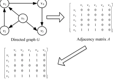
Figure 1. Warshall algorithm analysis diagram.

As showed in Figure 1 in the directed graph G, the connection between the nodes is represented by a straight line with an arrow, which intuitively reflects the connection.

However, it is difficult to determine the connection of the two non-connected points. The information passed by the matrix determines the connection of the nodes. The adjacency matrix A is a direct expression of the directed graph G, which is a direct connection of the directed graph G, with 1 and 0 indicating connectivity and disconnection, respectively. All reach cases of the directed graph G is listed in the reachable matrix F. Converting the adjacency matrix A into the reachable matrix F is implemented by the Warshall algorithm.

3.2. Warshall Algorithm

The Warshall algorithm proposed by Warshall in 1962 is a classical method based on binary relational transitive closure and is widely used. The steps of the Warshall algorithm are as follows:

Step 1: Set matrix A : = M

Step 2: Set i : 1 = ;

Step 3: For any j, if A[j,i]=1, then,

[ , ]

[ , ]

[ , ] among them,

1, 2, 3,...,

;

Step 4: i plus 1;

Step 5: If i ≤ n i, go to Step 2;

Step 6: The algorithm ends.

The reachable matrix only considers whether there is a road between v

. If it exits with 1 and does not exist, it is represented by 0.

3.3. The Basic Idea of W-DBSCAN Algorithm

A matrix of

[

] is established for n data in the data object set D, and the distance dis [i] [j] of the data object i and the data object j is calculated. If the value of dis [i] [j] is less than or equal to Eps, the matrix is obtained. The value of the position A [i, j] is marked as 1, similar to the adjacency matrix of the directed graph G in Figure 1., and the maximum density contiguous set of all data is obtained by the Warshall algorithm, which is similar to the Figure 1. reachable matrix F.

form. Then classify the data set. If the point m is not classified into any class, first determine whether the point m is the core point. If not, it is treated as noise; if it is, it is classified as C, and then the point m is found. The closure collection, the data in its closure collection is assigned to class C. C plus 1, enters the establishment of the next cluster, and so on, after all clusters are established, the algorithm ends.

1 2 3 4 5

1

2

3

4

5

0 0 0 1 0

1 0 0 0 0

0 0 0 0 0

0 0 1 0 0

1 1 1 0 0

v v v v v

v v v v v

 

 

 

 

 

 

 

 

 

 

1 2 3 4 5

1 2 3 4 5

0 0 1 1 0

1 0 1 1 0

0 0 0 0 0

0 0 1 0 0

1 1 1 1 0

v v v v v

v v v v v

 

 

 

 

 

 

 

 

 

 

3.4. Main Steps of the W-DBSCAN Algorithm

Step 1: Create matrix A for data object set D;

Step 2: Calculate dis [i] [j], if dis [i] [j]

j]=1, otherwise 0, establish an adjacency matrix;

Step 3: Using the Warshall algorithm to find the reachable matrix of the adjacency matrix, called the largest transitive closure set or the maximum density connected set;

Step 4: C++;

Step 5: Until all the data are ended by the clustering algorithm.

3.5. Flow Chart of W-DBSCAN Algorithm

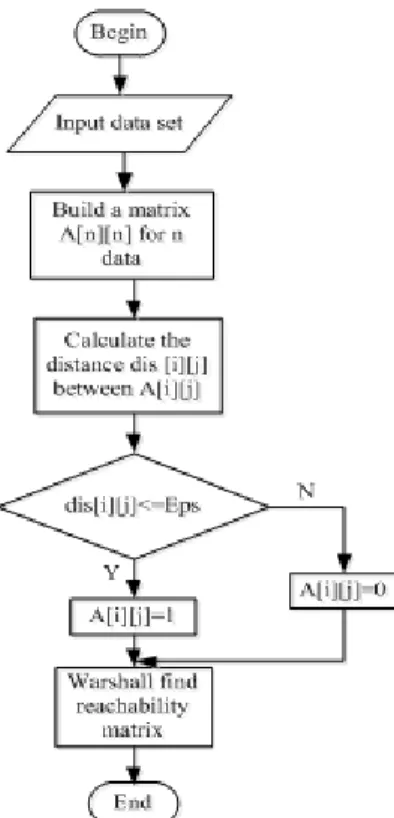
Figure 2. W-dbscan algorithm flowchart.

Figure 2 shows the flow chart of the W-DBSCAN algorithm.

The Warshall algorithm calculates the reachable matrix, that is, the density-connected set, and implements clustering. The clustering process is simpler than traditional density clustering.

Import the data set that needs data analysis, and establish the corresponding matrix, compare the distance between the two data with Eps, mark the established matrix as 0 and 1, 0 means that the distance between the two data is greater than Eps, 1 means The distance between the two data is less than or equal to Eps. For the matrix established above, through the Warshall algorithm analysis, the reachable data of the data set is obtained, and the data set can be the same category, and the data set is clustered.

4. The Analysis of Result

The proposed algorithm W-DBSCAN is written in language of C and MATLAB visualizes the simulation results. The

proposed algorithm is evaluated and analyzed through clustering results of discrete scale data sets.

4.1. Visual Dataset Experiment Results and Analysis

In order to verify the correctness of the proposed algorithm, the resulting algorithm is visually analyzed. In this experiment, three sets of two-dimensional data sets are gathered for visual analysis, and the W-DBSCAN algorithm is compared with DBSCAN, K-means and FCM algorithms respectively. As showed in Figure 3. Spiral data sets are clustered by DBSCAN, K-means, and FCM algorithms respectively. It can be seen from the figure that the clustering results of the FCM and W-DBSCAN algorithms are correct, and the K-means algorithm will The distances in the spiral data are divided into one class, which does not reflect the "spiral", because K-means only clusters convex data sets, can not cluster non-convex data sets, and the Spiral data sets are spiral non-convex data. Set; in Figure 4. is the graphical clustering result of the data set Flam on four algorithms. The clustering result of the data set only on the W-DBSCAN algorithm is correct, and the clustering on the K-means and FCM algorithms There is a problem, because the FCM algorithm is fuzzy clustering, the K-means algorithm only clusters the convex dataset; in Figure 5. the clustering of the dataset Aggregation on the four algorithms is the same as Figure 4.

because DBSCAN algorithm inherits the advantages of the DBSCAN algorithm and implements clustering of any type of data set. Table 1. shows the purity values of the three sets of data set on the W-DBSCAN, FCM, and K-means algorithms.

Boldness indicates that the clustering effect is better than other algorithms. As Table 1 the W-DBSCAN algorithm has the highest purity value, stable clustering effect, and better clustering results.

Table 1. Comparison of purity values in artificial data set.

Data Set W-DBSCAN FCM K-means

Sprial 1.00 0.95 0.33

Flame 1.00 0.99 0.85

Aggregation 1.00 0.72 0.72

4.2. UCI Dataset Experimental Results and Analysis

In order to verify the performance of W-DBSCAN, the above artificial data sets and UCI data sets were accurately quantified. Four sets of data were randomly selected from the UCI database and tested by W-DBSCAN, DBSCAN and FCM algorithms respectively. The first set of data: Iris, contains 150 data, 4 features, 3 categories; the second set of data Cmc:

contains 1473 data, 9 features, 3 categories; the third set of data Seeds: contains 210 data, 7 features, 3 categories; 4th set of data Tae: contains 151 data, 5 features, 3 categories. The data taken is from the text document, which is marked data.

The purity value [16] is selected as the index to measure the

accuracy of the clustering result of the algorithm. The value of

purity is between 0 and 1. The closer to 0, the more accurate

the data are Low, the closer to 1 the higher the accuracy of the

data.

Figure 3. Experimental results of the data set Spiral on four algorithms.

Figure 4. Experimental results of the data set Flam on four algorithms.

Figure 5. Experimental results of the data set Aggregation on four algorithms.

Table 2 shows the purity values of the four sets of data sets randomly selected from the UCI database on the W-DBSCAN, DBSCAN, and FCM algorithms. Boldness indicates that the clustering effect is better than other algorithms. Table 2 shows that the purity value on the Iris and Tae datasets is the largest on the W-DBSCAN algorithm, while the clustering effect of the Cmc and Seeds datasets is better than the W-DBSCAN algorithm, and the clustering effect of the Tae and Cmc datasets. Not so good because the two types of data sets have a large feature value owing to one of them, which affects the clustering result.

Table 2. Comparison of purity values in UCI data set.

Data Set W-DBSCAN FCM K-means

Iris 0.93 0.88 0.78

Tae 0.54 0.46 0.36

Cmc 0.66 0.52 0.35

Seeds 0.91 0.87 0.74

4.3. Algorithm Performance Analysis

Compared with DBSCAN, W-DBSCAN establishes the similarity matrix of the dataset, and uses the Warshall algorithm to find the density of the algorithm is reachable. It is not appropriate to judge the core points of each data object, and find any two from the similarity matrix. The path between the data and the non-zero path can find the density reachable path connected to the path, and realize the clustering of the data set. It can be viewed on the above analysis that the clustering results are stable and accurate, and the clustering efficiency is high.

Figure 6. Spiral data set.

In order to verify the running time of the algorithm, the artificial "helical data" is used for experiments, and the code is written with MATLAB tools to generate a spiral data set as showed in Figure 6. Depending on the data intensity and the number of data sets, similar shapes and different scales are generated. Density data set. Experiments with W-DBSCAN and DBSCAN with discrete scale data sets, and the running time diagram shown in Figure 7 is obtained. It can be observed in the figure that the W-DBSCAN algorithm runs faster than the DBSCAN algorithm.

Figure 7. Run time.

5. Conclusion

The density clustering algorithm is critical to the algorithm.

The algorithm of using the Warshall algorithm to solve the density connection is proposed. Firstly, the similarity matrix of the data object set is established, and then the reachable data object is calculated by the Warshall algorithm. Set is a class.

The Warshall algorithm is simple in process and low in complexity, making density clustering easier. The Warshall algorithm establishes a reachable matrix to cluster data object sets, reducing complexity. However, when establishing a matrix, it is judged that the similarity depends on the selection of the Eps value. If the selection value is too big or too small, the data object set will be more or less classified, and the clustering is incorrect. Therefore, the next step will be tantamount to design global threshold calculations to reduce external interference with clustering.

Fund

2018 Guangdong Province "Innovative Strong School Project" Scientific Research Project Research on the construction of data visualization platform (2017KQNX266).

References

[1] TU Q, LU J F, YUAN B, et al. Density-based hierarchical clustering for streaming data [J]. Pattern Recognition Letters, 2012, 33 (5): 641-645.

[2] LIU Q, DENG M, SHI Y, et al. A density-based spatial clustering algorithm considering both spatial proximity and attribute similarity [J]. Computers & Geosciences, 2012, 46 (3):

296-309.

[3] J G Sun, J Liu, L Y Zhao. Research on Clustering Algorithm [J].

Journal of Software, 2008, 19 (01): 48-61.

[4] S G Zhou, A Y Zhou. A fast clustering algorithm based on density [J]. Computer research and development, 2000, 37 (11):

1287-1292.

[5] ESTER M, KRIEGEL H P, XU X. A density-based algorithm

for discovering clusters a density-based algorithm for discovering clusters in large spatial databases with noise [C]//

International Conference on Knowledge Discovery and Data Mining. AAAI Press, 1996: 226-231.

[6] BIRABT D, KUT A. ST-DBSCAN: An Algorithm for Clustering Spatial-temporal Data [J]. Data and Knowledge Engineering, 2007, 60 (1): 208-221.

[7] Z H Feng, X Z QIAN, N N Zhao. Greedy DBSCAN: An Improved DBSCAN Algorithm for Multi-Density Clustering [J]. Application Research of Computers, 2106 (9):

2693-2696.

[8] Z F Wang, G L Shan. Method for dynamically selecting parameters of DBSCAN algorithm based on k-means [J].

Computer Engineering and Applications, 2017, 53 (03): 80-86.

[9] Y Cai, J S Yuan. Text clustering based on improved DBSCAN algorithm [J]. Computer Engineering, 2011, 37 (12): 50-52.

[10] S G Zhou, A Y Zhou, J Cao. DBSCAN algorithm based on data partition [J]. Computer research and development, 2000, 37 (10): 1153-1159.

[11] G Li, H B Liu, Y Feng. Clustering method based on λ-Warshall algorithm [J]. Computer Engineering and Design, 2008, 29 (8):

1903-1904.

[12] MACQUEEN J. Some Methods for Classification and Analysis of MultiVariate Observations [C]// Proc. of, Berkeley Symposium on Mathematical Statistics and Probability. 1967:

281-297.

[13] WARSHALL S. A Theorem on Boolean Matrices [J]. Journal of the Acm, 1962, 9 (1): 11-12.

[14] BREUNIG M, KRIEGEL H P, NG R, etal. LOF: Identifying Density- based Local Outliers [C]//Proc. of ACM SIGMOD International Conference on Management of Data. [S. l.]: ACM Press, 2000.

[15] F Z Sun, Y H Li, S M Cheng etal. Application of Warshall algorithm in discriminating transitivity and seeking transitive closure [J]. Journal of Changchun University, 2007, 17 (6):

13-16.

[16] YANG Z, OJA E. Linear and Nonlinear Projective Nonnegative Matrix Factorization [J]. IEEE Trans Neural Netw, 2010, 21 (5): 734-749.