AMF-IDBSCAN: Incremental Density Based Clustering Algorithm
using Adaptive Median Filtering Technique
Aida Chefrour and Labiba Souici-Meslati
LISCO Laboratory, Computer Science Department, Badji Mokhtar-Annaba University PO Box 12, Annaba, 23000, Algeria
Computer Science Department, Mohamed Cherif Messaadia, Souk Ahras, Algeria E-mail: [email protected], [email protected]
Keywords: incremental learning, DBSCAN, canopy clustering, adaptive median filtering, f-measure
Received: December 28, 2018
Density-based spatial clustering of applications with noise (DBSCAN) is a fundamental algorithm for density-based clustering. It can discover clusters of arbitrary shapes and sizes from a large amount of data, which contains noise and outliers. However, it fails to treat large datasets, outperform when new objects are inserted into the existing database, remove noise points or outliers totally and handle the local density variation that exists within the cluster. So, a good clustering method should allow a significant density modification within the cluster and should learn dynamics and large databases. In this paper, an enhancement of the DBSCAN algorithm is proposed based on incremental clustering called AMF-IDBSCAN which builds incrementally the clusters of different shapes and sizes in large datasets and eliminates the presence of noise and outliers. The proposed AMF-IDBSCAN algorithm uses a canopy clustering algorithm for pre-clustering the data sets to decrease the volume of data, applies an incremental DBSCAN for clustering the data points and Adaptive Median Filtering (AMF) technique for post-clustering to reduce the number of outliers by replacing noises by chosen medians. Experiments with AMF-IDBSCAN are performed on the University of California Irvine (UCI) repository UCI data sets. The results show that our algorithm performs better than DBSCAN, IDBSCAN, and DMDBSCAN.
Povzetek: V članku je predstavljen nov algoritem AMF-IDBSCAN, izboljšana različica DBSCAN, ki uporablja grozdenje krošenj za zmanjšanje obsega podatkov in tehnike AMF za odpravo hrupa.
1
Introduction
Data mining is an interdisciplinary topic that can be defined in many different ways [1]. In the field of database management industry, data analysis is mainly concerned with a number of large data repositories and aims to identify valid, useful, novel and understandable patterns in the existing data.
Clustering is a principal data finding technique in data mining. It separates a data set into subsets or clusters so that data values in the same cluster have some common characteristics or attributes [2]. It aims to divide the data into groups (clusters) of similar objects [3]. The objects in the same cluster are more identical to each other than to those in other clusters. Clustering is widely used in Artificial Intelligence, Pattern recognition, statistics, and other information processing fields.
Many clustering algorithms have been progressed; they may be divided into the following major categories [4]: hierarchical clustering algorithms (BIRCH, CHAMELEON,..), partitioning algorithms (means, K-medoids), density-based algorithms (DBSCAN, OPTICS) and grid-based algorithms (STING, CLIQUE). The input of a cluster analysis system is a set of samples and a measure of similarity (or dissimilarity) between two samples. The output is a set of clusters that form a partition, or a structure of partitions of the data set. Generally, finding clusters is not a simple task and
the current clustering algorithms take much time when they are applied to large databases.
In addition, most of the databases are dynamic in nature, data is inserted and deleted from them frequently. The static clustering does not process this kind of databases that’s why the concept of incremental clustering was introduced and used.
The difference between the traditional clustering methods (batch mode) and those of incremental clustering is the ability of the latter to process new data included in the data collection without having to perform a full re-clustering. This allows a dynamic following of updates to the database during clustering.
Incremental learning is a research area that received great attention in recent years since it allows effective reuse of data, fast and pragmatic learning based on context, augmentation of knowledge, learning in dynamic and large databases, exploration and smart decision making [5].
and parametrically through different data-driven mechanisms [7].
In our study, we focus on the DBSCAN (Density-Based Spatial Clustering of Applications with Noise) clustering algorithm. The core idea of DBSCAN is that each object within a cluster must have a certain number of other objects in its neighborhood. Compared with other clustering algorithms. DBSCAN has many attractive benefits and was used by many researchers in recent years with its several extensions and applications.
We were particularly interested in the incremental version of DBSCAN since (1) it is capable of discovering clusters of random shape; (2) it requires just two parameters and is most inconsiderate to the ordering of the points in the database; (3) it reduces the search space and facilitates an incremental update in the clusters; (4) it is more adaptive to various datasets and data space without some initial information [8] and (5) the DBSCAN with incremental concept saves a lot of time and effort efficiently, whereas static DBSCAN has already suffered from some drawbacks and these problems are mainly faced in dynamic large databases in the existing system [9];
In this paper, we propose an AMF-IDBSCAN algorithm an enhanced version of the DBSCAN. Our algorithm consists of three main phases. After importing the original database, it preprocesses it to prepare the clustering step and to reduce the volume of the dataset using Canopy clustering. Then, the classical DBSCAN algorithm is applied to the results of the first step to produce another database. Next, the incremental DBSCAN algorithm is applied to the incremental dataset. The adaptive median filtering technique is applied to the results of the previous step to remove noise and outliers. Then, the results are compared and the performance is evaluated.
The rest of the paper is organized as follows. In the next section, we survey in brief the literature of enhanced DBSCAN algorithms. In Section 3, we describe in details our contribution to AMF-IDBSCAN. Section 4 describes the experiment we conducted and the results obtained by our algorithm. It also compares them with top-ranked algorithms. Finally, we draw some conclusions and show ongoing research aspects in Section 5.
2
Related work
Several algorithms for improvements of DBSCAN exist in the literature. In this section, we outline the best known and most recent ones. We noticed that all of these algorithms have shown good results, in the last few years. However, no one of them could be said to be the best but all depend on the content of input parameters and their application domain:
DVBSCAN (A Density-Based Algorithm for Discovering Density Varied Clusters in Large Spatial Databases) [10] is an algorithm which handles local density variation within the cluster. The following input parameters are introduced: minimum objects (μ), radius, and threshold values (α, λ), to calculate the growing cluster density mean and the cluster density variance for
any core object, which appears to be developed further by considering the density of its Neighborhood with respect to cluster density mean. A comparison between a cluster density variance for a core object and a threshold value is affected if the first is less than the second and is also satisfying the cluster similarity index, and then it will allow the core object for expansion.
ST-DBSCAN (Spatial-Temporal Density-Based Clustering) [11] is constructed to improve the DBSCAN algorithm by introducing the ability to discover clusters with respect to spatial, non-spatial, and temporal values of the objects. ST-DBSCAN works in three stages: (1) It can cluster spatial-temporal data according to spatial, non- spatial, and temporal attributes. (2) To resolve the problem of no detection of the noise input in DBSCAN, ST-DBSCAN assigns density factor to each cluster. (3) To solve the conflicts in border objects, it compares the average value of a cluster with new coming value.
VDBSCAN (Varied Density-Based Spatial Clustering of Applications with Noise) [12] is a new improvement to DBSCAN, it detects cluster with a varied density as well as automatically selects several values of input parameter Eps for different densities. It has a two-step procedure. In the first step, the values of
Eps are calculated for different densities according to a K-dist. plotting. These calculated values are then further used to analyze the clusters with different densities. In the second step, the DBSCAN algorithm is applied with the parameter Eps values calculated in the previously discussed step. It ensures that all of the clusters with corresponding densities are clustered.
VMDBSCAN (Vibration Method DBSCAN) [13] is designed for modifying the DBSCAN algorithm. Unlike to existing density-based clustering algorithm, it detects the clusters of different shapes, sizes that differ in local density. VMDBSCAN first extracts the “core” of each cluster after applying DBSCAN. Then it “vibrates" points towards the cluster that has the maximum effect on these points.
DMDBSCAN (Dynamic Method DBSCAN) [14] is a new enhancement of DBSCAN which has pointed out that in clusters, generated by DBSCAN, there is wide density variation. Compared to DBSCAN which uses global Eps. It has successfully given the method to compute Eps automatically for each of the different density levels in the dataset based on k-dist. plot. The major success of this technique includes (1) easy interpretation of generated clusters; (2) no limit on the shape of the generated clusters. DMDBSCAN will use the dynamic method to find a suitable value of Eps for each density level of data set.
perform density-based clustering on this prototype respectively.
GRIDBSCAN [16] is another important variation of DBSCAN that addresses the issue that exists in most of the density-based clustering algorithms, which is the lack of accurate clustering in the presence of clusters with different densities. It has a three-level mechanism. In the first level, it provides appropriate grids such that density is similar in each grid. In the next level, it merges the cells having the same densities. At this level, the appropriate value of 𝐸𝑝𝑠 and MinPts are also identified in each grid. In the final step, the DBSCAN algorithm is applied to these identified parameters values to obtain the required final number of clusters.
FDBSCAN (Fast Density-Based clustering algorithm for large Database) [17] is an improved version of DBSCAN clustering. This was developed to overcome: (1) its slow speed (slow in comparison due to neighborhood query for each object); (2) and setting the threshold value of the DBSCAN algorithm. The FDBSCAN starts by ordering the dataset object by certain dimensional coordinates. Then it considers a point having a minimal index and retrieves its neighborhood. If this point is demonstrated as a core object then a new cluster is created to label all objects in its neighborhood. In this way, the next unlabeled point is analyzed outside the core object to expand clusters. When all the points are analyzed for clustering then these objects are further passed through a Kernel function. This will ensure the distribution of object as uniform as possible.
MR-DBSCAN [18] is a parallel version of DBSCAN in a MapReduce manner. It provides a method to divide a large dataset into several partitions based on the data dimensions. In the map phase, localized DBSCANs can be applied to each partition in parallel. During a final reduce phase, the results of each partition are then merged. For the overall cost, a partition-division phase is added into DBSCAN. A Cost Balanced Partition division method is used to generate partitions with equal workloads. This parallel extension meets the requirements of scalable execution for handling large-scale data sets and the MapReduce approach makes it suitable for many popular big data analytics platforms like Hadoop MapReduce and ApacheSpark.
M-DBSCAN (Multi-Level DBSCAN) [19] is an algorithm where neighborhood is not defined by a constant radius. Instead, the definition of the neighboring radius is performed based on the data distribution around the core using standard deviation and mean values. To obtain the clustering results, M-DBSCAN is applied on a set of core-mini clusters where each core-mini cluster defines a virtual point which lies in the center of that cluster. In M-DBSCAN, the value of DBSCAN is replaced by local density cluster which the clusters are extended by adding core-mini clusters that have similar mean values with a little difference determined by the standard deviation of the core.
FI-DBSCAN [20] is a Frequent Itemset Ultrametric Trees with Density Based Spatial Clustering of
Applications with Noise (DBSCAN) on MapReduce framework is used in the proposed system to solve the evolution and efficiency problem in an existing frequent itemset. It incorporates the Density Based Frequent Itemset Ultrametric Tree by adding additional hash tables rather than using conventional FP trees, there are by achieving compressed storage and avoiding the necessity to build conditional pattern bases. FI-DBSCAN integrates three MapReduce jobs to accomplish parallel mining of frequent itemsets. The first MapReduce job is responsible for mining all frequent one- itemsets. The second MapReduce job applies the second round of analyzing the database to eliminate infrequent items from each transaction record. At the end of the third MapReduce job, all frequent K-itemsets are created.
AnyDBC (An Efficient Anytime Density-based Clustering Algorithm for Very Large Complex Datasets) [21] is an anytime algorithm which requires very small initial runtime for acquiring similar results as DBSCAN. Thus, it not only allows user interaction but also can be used to obtain good approximations under arbitrary time constraints.
IDBSCAN [22] proposes an enhanced version of the incremental DBSCAN algorithm for incrementally building and updating arbitrarily shaped clusters in extensive datasets. The proposed algorithm ameliorates the incremental clustering process by limiting the search space to partitions instead ofthe whole dataset, and this gives significant improvements in performance compared to relevant incremental clustering algorithms. To enhance this algorithm further, [23] proposes an incremental DBSCAN which is fused with a suitable noise removal and outlier detection technique inspired by the box plot method. It utilizes a between network measure to dense regions to frame the last number of clusters.
3
The proposed AMF-IDBSCAN
clustering algorithm
To overcome the limitations of the high complexity and the non scalability of the traditional clustering algorithms, we have developed in this work AMF-DBSCAN: An enhanced incremental DBSCAN using a canopy clustering algorithm and an adaptive median filtering technique.
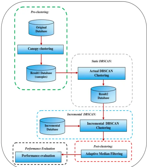
The proposed AMF-IDBSCAN consists of four phases as shown in Figure 1. The first phase is pre-clustering employing Canopy pre-clustering. The second phase is the clustering of data objects in which Incremental DBSCAN is used. The third phase is post-clustering applying Adaptive Median Filtering method that aims to reduce the number of outliers by replacing them with chosen medians. The last phase is used to evaluate the performance of clustering algorithms using different evaluation metrics:
Pre-clustering:
Original Database
Canopy clustering
Adaptive Median Filtering Performance evaluation
Incremental Database
Actual DBSCAN Clustering
Incremental DBSCAN Clustering
Result1 Database (canopies)
Result2 Database Static DBSCAN:
Incremental DBSCAN:
Performance Evaluation Post-clustering:
Figure 1: The methodology of the proposed incremental AMF-IDBSCAN clustering algorithm.
3.1
Pre-clustering
This step is aims to prepare the clustering. We used the canopy clustering algorithm which is an unsupervised pre-clustering algorithm introduced by [24]. We have chosen a canopy clustering method for pre-processing the data because (1) it is efficient when the problem is large (2) it can greatly reduce the number of distance computations required for clustering by first cheaply partitioning the data into overlapping subsets, and then only measuring distances among pairs of data points that belong to a common subset and (3) it tries to speed up the clustering of large data sets that are a high dimension by dividing the clustering process into two subprocesses, where using another algorithm directly may be impractical due to the size of the data set (see Figure 2).
First, the data set is divided into overlapping subsets called canopies. This is done by choosing a distance metric and two thresholds, T1 and T2, where T1 > T2.
All data points are then added to a list and one of the points in the list is picked at random. The remaining points in the list are iterated over and the distance to the initial point is calculated. If the distance is within T1, the point is added to the canopy. Further, if the distance is
within T2, the point is removed from the list. The algorithm is iterated until the list is empty.
The output of the Canopy clustering is the input of static DBSCAN;
3.2
Classical static DBSCAN clustering
algorithm
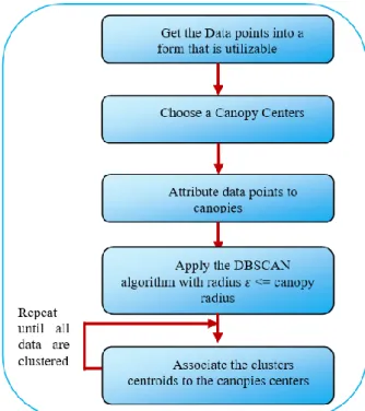
When used with canopy clustering, the DBSCAN algorithm can reduce the computations in the radius (Eps) calculation step that delimits the neighborhood area of a point hence improving the efficiency of the algorithm. The implementations of the DBSCAN algorithm with Canopy Clustering involves the following steps (see Figure 3):
Figure 3: DBSCAN algorithm with Canopy Clustering. 1. Prepare the data points: the input data needs to be
transformed into a format suitable and utilizable for distance and similarity measures.
2. Choose Canopy Centers
3. Attribute data points to canopy centers: the canopy assignment step would simply assign data points to generated canopy centers.
4. Associate the cluster's centroids to the canopies centers. The data points are now in clustered sets. 5. Repeat the iteration until all data are clustered. 6. Apply the DBSCAN algorithm with radius 𝜀<=
canopy radius and iterate until clustering. The computation to calculate the minimum number of points (Minpts) is greatly reduced as we only calculate the distance between a clusters centroids and data point if they share the same canopy. 7. DBSCAN is a widely used technique for clustering
in spatial databases. DBSCAN needs less knowledge of input parameters. The major advantage of DBSCAN is to identify arbitrary shape objects and removal of noise during the clustering process. Besides its familiarity, it has problems with handling large databases and in the worst case, its complexity reaches to O(n2)[26]. Additionally, DBSCAN cannot produce a correct result on varied
densities. That's why we used canopy clustering in our case to reduce its complexity:
In the AMF-IDBSCAN algorithm, we partition the data (n is the number of data) into canopies C by canopy clustering, each containing about (n / C) points. Then the complexity will decrease to (n2 /C) for the AMF-IDBSCAN algorithm.
In the sub-section, we describe the static DBSCAN: The static DBSCAN algorithm was first introduced by [27]. It uses a density-based notion of clustering of arbitrary shapes, which is designed to discover clusters of arbitrary shape and also has the ability to handle noise. It relies on the density-based notion of clusters. Clusters are identified by looking at the density of points.
Regions with a high density of points depict the existence of clusters, whereas regions with a low density of points indicate clusters of noise or clusters of outliers. The key idea of the DBSCAN algorithm [28] is that, for each point of a cluster, the neighborhood of a given radius has to contain at least a minimum number of points, that is, the density in the neighborhood has to exceed some predefined threshold. This algorithm needs two input parameters:
Eps, the radius that delimits the neighborhood area of a point (Eps-neighborhood);
MinPts, the minimum number of points that must exist in the Eps-neighborhood.
The clustering process is based on the classification of the points in the dataset as core points, border points, and noise points, and on the use of density relations between points (directly reachable, density-reachable, density-connected) to form the clusters (see Figure 4).
Core point: lies in the interior of density based clusters and should lie within Eps (radius or threshold value), MinPts (minimum number of points) which are user-specified parameters.
Border point: lies within the neighborhood of core point and many core points may share the same border point.
Noise point: is a point which is neither a core point nor a border point.
Directly Density-Reachable: a point P is directly density-reachable from a point Q with respect to (w.r.t) Eps, MinPts if P belongs to NEps(Q) |NEps (Q)| >= MinPts
Density-Reachable: a point P is density-reachable from a point Q w.r.t Eps, MinPts if there is a chain of points P1, …, Pn, P1 = Q, Pn = P such that Pi+1 is directly density-reachable from Pi
Density-Connected: a point P is density-connected to a point Q w.r.t Eps, MinPts if there is a point O such that both, P and Q are dense-reachable from O w.r.t Eps and MinPts.
Figure 4: DBSCAN working.
3.3
Incremental DBSCAN clustering
The static DBSCAN approach is not suitable for a large multidimensional database which is frequently updated. In that case, the incremental clustering approach is much finer. In our study, we use incremental DBSCAN to enhance the clustering process by incrementally partitioning the dataset to reduce the search space of the neighborhood to one partition rather than the whole data set. Also, it has embedded flexibility regarding the level of granularity and is robust to noisy data.We have chosen as a foundation of our incremental DBSCAN clustering algorithm, the algorithm of [29] which works in two steps:
Step 1. Compute the means between every core object of the clusters and the new data. Insert the new data into a specific cluster based on the minimum mean distance. Sign the data as noise or border if it cannot be inserted into any clusters.
Step 2. Form new core points or clusters when noise points or border points fulfill the Minpts (the minimum number of points) and radius criteria.
Sometimes DBSCAN may be applied on a dynamic database which is frequently updated by the insertion or deletion of data. After insertions and deletions to the database, the clustering located by DBSCAN has to be updated. Incremental clustering could enhance the chances of finding the global optimum. In this approach,
first, it will form clusters based on the initial objects and a given radius (eps) and Minpts. Thus the algorithm finally gets some clusters fulfilling the conditions and some outliers. When new data is inserted into the existing database, we have to update the existing clusters using DBSCAN. At first, the algorithm computes the means between every core object of clusters and the new coming data and insert it into a particular cluster based on the minimum mean distance. The new data which is not inserted into any clusters, is treated as noise or outlier. Sometimes outliers which fulfill the Minpts & Eps criteria, combined can form clusters using DBSCAN.
We have used the Euclidean distance because it is currently the most frequently used metric space for the established clustering algorithms [30].
The steps of incremental DBSCAN clustering algorithm are as follows:
Pseudo-code of incremental DBSCAN
Input
D: a dataset containing n objects {X1,X2, X3 …, Xn}; n: number of data items;
Minpts: Minimum number of data objects ; eps: radius of the cluster.
Output
K: a Set of clusters.
Procedure
Let, Ci (where i=1, 2, 3 …) is the new data item. 1. Run the actual DBSCAN algorithm and clustered the new data item Ci properly based on the radius(eps) and the Minpts criteria. Repeat till all data items are clustered.
Incremental DBSCAN Pseudo-code: Start:
2. a> Let, K represents the already existing clusters. b>When new data is coming into the database, the new data will be directly clustered by calculating the minimum mean(M) between that data and the core objects of existing clusters.
for i = 1 to n do
find some mean M in some cluster Kp in K such that dis ( Ci, M ) is the smallest; If (dis ( Ci, M ) is minimum) && (Ci<=eps) && (size(Kp)>=Minpts) then
Kp = Kp U Ci ; Else
If dis (Ci != min) || (Ci>eps) ||(size(Kp)<Minpts) then Ci Outlier(Oi) .
Else
If Count(Oi) Minpts then Oi Form new cluster(Mi). C > Repeat step b till all the data samples are clustered. End.
3.4
Post-clustering
We illustrate the clusters and the outliers points by a rectangular window 𝑊on a hyperplane of n dimensions equivalent to the data dimensions. We apply the Adaptive Median Filtering (AMF) to reduce the noise
2 1 0 1 2
-1.5 -1 -0.5
-0 0.5 1 1,5 2
Eps=1
Noise Point
Border Point Core Point
MinPts=4 • Arbitrary select a point P
• Retrieve all points density-reachable from P w.r.t Eps and MinPts.
• If P is a core point, a cluster is formed.
• If P is a border point, no points are dense-reachable from P and DBSCAN visits the next point of the database.
data. We have taken the key idea of this method and we have applied it to our proposition. This is an important advantage of our approach.
We have selected Adaptive Median Filtering (AMF) among various filtering techniques because it removes noise while preserving shape details [31]. AMF technique is used to replace the outliers generated by incremental DBSCAN by a cluster contains an object.
The adaptive median filtering [32] has been widely applied as an advanced method compared with standard median filtering. The adaptive filter works on a rectangular region 𝑊 (illustration of the set of clusters and outliers generated by the previous stage on a hyperplane). It changes the size of W during the filtering operation depending on certain criteria as listed below. The output of the filter is a single value which replaces the current noise data value at (x, y,....), the point on which 𝑊 is centered at the time.
Let Ix,y,...be the selected noise data according to the dimensions, Imin be the minimum noise value and Imax be the maximum noise value in the window, W be the current window size applied, Wmax be the maximum window size that can be achieved and Imed be the median of the window designated. The algorithm of this filtering technique completes in two levels as described in [33]:
Level A:
a) If Imin< Imed< Imax then the median value is not an impulse, so the algorithm goes to Level B to check if the current noise is an impulse.
b) Else the size of the window is increased and Level A is repeated until the median value is not a stimulus so the algorithm goes to Level B; or the maximum window size is reached, in which case the median value is assigned as the filtered selected noise value.
Level B:
a) If Imin < Ix,y,.... < Imax, then the current noise value is not a stimulus, so the filtered selected noise is unchanged b) Else the selected noise data is either equal to Imax or Imin, then the filtered selected noise data is assigned the median value from Level A.
These types of median filters are widely used in filtering data that has been denoised with noise density greater than 20%.
This technique has three main purposes:
• To remove noise;
• To smoothen any non-stimulus noise;
• To reduce excessive shapes of clusters
3.5
Performance evaluation
To evaluate the performance of our approach, the canopies are applied to the original dataset and store the result into another database, and then the actual DBSCAN algorithm is applied to the results to this database. The incremental DBSCAN algorithm is applied to the incremental dataset. The results of these two algorithms are compared and their performances are evaluated.
The proposed algorithm AMF-IDBSCAN is shown as pseudo-code in Algorithm 2:
Pseudo-code of AMF-IDBSCAN
Input
D: a dataset containing n objects {X1,X2, X3 …, Xn}; n: number of data items;
Minpts: Minimum number of data objects ; eps: radius of the cluster.
CN: canopies centers
Output
K: a Set of clusters. A single value: Ix,y,.... or Imed
Procedure
1. Run Canopy clustering :
1.1. Put all data into a List, and initialize two distance radius about the loose threshold T1 and the tight threshold T2 (T1> T2).
1.2. Randomly select a point as the first initial center of the Canopy cluster, and delete this object from the List.
1.3. Get a point from the List, and calculate the distance d to each Canopy clusters.
If d < T2, the point belongs to this cluster; if T2≤d≤T1, this point will be marked with a weak label; If the distance d to all Canopy center is greater than T1, then the point will be classed as a new Canopy cluster center. Finally, this point should be eliminated from the List;
1.4. Run the step1.3 repeatedly until the list is empty, and recalculate the canopy centers CN.
2. Run the actual DBSCAN algorithm and clustered the new data item Ci properly based on the radius(eps) and the Minpts criteria. Repeat till all data items are clustered:
2.1. Choosing Canopy Centers CN
2.2. Attribute data points D to canopy centers CN; 2.3. Apply the DBSCAN algorithm with radius
𝜀
<= canopy radius with dist(CN, Ci)<Minpts2.4. Repeat the iteration until all data are clustered. 3. Run the incremental DBSCAN:
3.1. a> Let, K represents the already existing clusters. 3.2. When new data is coming into the database, the new data will be directly clustered by calculating the minimum mean(M) between that data and the core objects of existing clusters.
For i = 1 to n do
find some mean M in some cluster Kp in K such that dis ( Ci, M ) is the smallest; If (dis ( Ci, M ) is minimum) && (Ci<=eps) && (size(Kp)>=Minpts) then
Kp = Kp U Ci ; Else
If dis (Ci != min) || (Ci>eps) ||(size(Kp)<Minpts) then Ci Outlier(Oi).
3.3. Elimination of noise objects Oi:
The new dataset contains Oi and the clusters closest to it.
Let:
Ix,y....be the selected noise data (Oi) at the coordinates (x,y,...); % corresponding the data dimensions; Imin be the minimum noise value;
Imax be the maximum noise value in the window; W be the current window size applied; % It contains K clusters and Oi
Wmax be the maximum window size that can be reached;
Imed be the median of the window assigned Algorithm
Level A: A1= Imed - Imin A2= Imed - Imax
If A1 > 0 AND A2 < 0, Go to level B Else increase the window size
If window size W<= Imax repeat level A Else output Ix,y...
Level B: B1 = Ix,y,.. – Imin B2 = Ix,y,..– Imin
If B1 > 0 And B2 < 0 output Ix,y,.. Else output Imed.
3.5. Repeat step b till all the data samples are clustered.
4. Evaluate performance.
4
Experiments and results
This section presents a detailed experimental analysis carried out to prove our proposed clustering technique AMF-IDBSCAN is better than other state of art methods used for high dimensional clustering. We have taken five high dimensional data sets (Adult, Wine, Glass identification, Ionosphere, and Fisher's Iris) from UC Irvine repository (refer Table 1) to test the performance in terms of F-measure, number of clusters, error rate, number of uncluttered instances and time is taken to build the model. F-measure is defined in equation (1), it is the harmonic average of precision and recall. It is a one only summary statistic that does not credit an algorithm for correctly placing the very large number of pairs into different clusters [34]. F-Measure is commonly used in evaluating the efficiency and the reliability of clustering and classification algorithms.
Our proposed noise removal and outlier labeling method are compared with static DBSCAN, an incremental density based clustering algorithm (IDBSCAN) [22], DMDBSCAN [14] presented below is the brief related work, about evaluation metrics used for evaluating clustering results:
𝐹 − 𝑚𝑒𝑎𝑠𝑢𝑟𝑒 =2×𝑃𝑟𝑒𝑐𝑖𝑠𝑖𝑜𝑛×𝑅𝑒𝑐𝑎𝑙𝑙
𝑃𝑟𝑒𝑐𝑖𝑠𝑖𝑜𝑛+𝑅𝑒𝑐𝑎𝑙𝑙 (1) 𝑊ℎ𝑒𝑟𝑒 ∶
𝑃𝑟𝑒𝑐𝑖𝑠𝑖𝑜𝑛 = 𝑇𝑃
𝑇𝑃+𝐹𝑃 (2) 𝑅𝑒𝑐𝑎𝑙𝑙 = 𝑇𝑃
𝑇𝑃+𝐹𝑁 (3)
Where TP: True positive, FP: False positive, FN: False negative
DBSCAN:
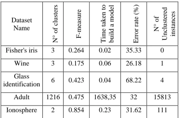
We apply the DBSCAN algorithm on wine dataset with Eps = 0.9 and MinPts = 6, F-measure= 0.175 and obtain an average error index of 26.18%, number of clusters = 3. While applying DBSCAN on Iris data set, we get an average error index of 35.33% with the same Eps and Minpts, F-measure= 0.264, number of clusters = 3. Another real data set is Glass dataset and when we apply DBSCAN on it, we get an average error index of 68.22 %, F-measure= 0.423 with a number of = 6. We get for Adult dataset an average error index of 32%, F-measure= 0.475 with number of clusters=1216. For ionosphere, an average error index= 31.62%, F-measure= 0.854 and number of clusters=2 (see Table 2)
Dataset Name
N° o
f
clu
ste
rs
F
-m
ea
su
re
Ti
m
e
tak
en
to
b
u
il
d
a
m
o
d
el
Err
o
r
ra
te (%
)
N° o
f
Un
clu
ste
re
d
in
sta
n
ce
s
Fisher's iris 3 0.264 0.02 35.33 0
Wine 3 0.175 0.06 26.18 1
Glass
identification 6 0.423 0.04 68.22 4
Adult 1216 0.475 1638,35 32 15813
Ionosphere 2 0.854 0.23 31.62 111
Table 2: Results of applying DBSCAN. IDBSCAN:
We apply IDBSCAN algorithm on wine dataset with Eps = 0.9 and MinPts = 6, F-measure= 0.274 and obtain an average error index of 23.45%, number of clusters = 4. While applying IDBSCAN on Iris data set, we get an average error index of 28.54% with the same Eps and Minpts, F-measure= 0.354, number of clusters = 3. Another real data set is Glass dataset and when we apply IDBSCAN on it, we get an average error index of 49.52%, F-measure= 0.323 with a number of clusters = 8. We get for Adult dataset an average error index of Dataset No. of
instances
No. of
attributes Attribute type Data types Ionosphere 351 34 Integer, real Multivariate
Wine 178 13 Integer, real Multivariate
Glass
Identification 214 10 Real Multivariate
Adult 48842 15 Categorical,
Integer, Real Multivariate
Fisher's Iris 150 4 Real Multivariate
27.96%, F-measure= 0.475 with number of clusters=1265. For ionosphere, an average error index= 29.15%, F-measure= 0.639 and number of clusters=3 (see Table3).
Table 3: Results of applying IDBSCAN. AMF-IDBSCAN:
In our experiments, we have used for canopy clustering implementation, a Weka tool (Waikato Environment for Knowledge Analysis) [35] which is an open-source Java application produced by the University of Waikato in New Zealand. It functions like Preprocessing Filters, Attribute selection, Classification/Regression, Clustering, Association discovery, Visualization. The set of training instances has to be encoded in an input file with.ARFF (Assign Relation File Format) extension to be used by the Weka tool in order to generate the canopies that will be used as inputs in our algorithm.
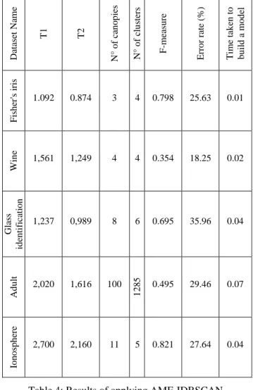
We apply our proposed AMF-IDBSCAN algorithm on wine data set with Eps = 0.9 and MinPts = 6, number of canopies= 4, F-measure= 0.354 and obtain an average error index of 18.25%, number of clusters = 4. While applying AMF-IDBSCAN on Iris data set, we get an average error index of 25.63% with the same Eps and Minpts, number of canopies= 3, F-measure= 0.758, number of clusters = 4. Another real data set is Glass data set and when we apply our proposed algorithm on it, we get an average error index of 35.96% , number of canopies= 8, F-measure= 0.695 with number of = 6. We get for Adult dataset an average error index of 29.46%, number of canopies= 100, F-measure= 0.495 with number of clusters=1285. For ionosphere, an average error index= 27.64%, number of canopies= 11, F-measure= 0.821 and number of clusters=5 (see Table 4).
DMDBSCAN:
We apply the DMDBSCAN algorithm on the wine data set, and applying k-dist for 3-nearest points, we have 3 values of Eps which are 4.3, 4.9 and 5.1. F-measure= 0.125, the average error index is 23.15% and number of clusters = 3. While applying DMDBSCAN on Iris data set, and applying k-dist for 3-nearest points, we have 2 values of Eps which are 0.39 and 0.45. The average error index is 38.46%, F-measure =0.295 and a number of clusters = 3.
Another real data set is Glass dataset and when we apply DMDBSCAN on it and applying k-dist for
3-nearest points, we have 3 values of Eps which are 0.89, 9.3 and 9.4. F-measure= 0.623, the average error index is 58.39% and the number of clusters = 6. We get for Adult dataset an F-measure= 0.474, the average error index of 34.66%, with a number of clusters=1301. For ionosphere, F-measure= 0.754, an average error index= 30.04%, and number of clusters=6 (see Table 5).
Da tas et Na m e T1 T2 N° o f ca n o p ies N° o f clu ste rs F -m ea su re Err o r ra te (% ) Ti m e tak en to b u il d a m o d el F ish er' s ir is
1.092 0.874 3 4 0.798 25.63 0.01
Wi
n
e
1,561 1,249 4 4 0.354 18.25 0.02
Gla ss id en ti fica ti o n
1,237 0,989 8 6 0.695 35.96 0.04
Ad
u
lt
2,020 1,616 100
1
2
8
5
0.495 29.46 0.07
Io n o sp h ere
2,700 2,160 11 5 0.821 27.64 0.04
Table 4: Results of applying AMF-IDBSCAN.
Dataset Name N° of clusters F-measure Error rate (%) Time is taken to build a model
Fisher's iris 3 0.293 38.46 0.08
Wine 3 0.125 23.15 0.13
Glass
identification 6 0.623 58.39 0.24
Adult 1301 0.474 34.66 0.64
Ionosphere 6 0.754 30.04 0.09
Table 5: Results of applying DMDBSCAN. Dataset Name N° of
clusters F-measure
Time taken to build a
model
Error rate (%)
Fisher's iris 3 0.354 0.03 28.54
Wine 4 0.274 0.05 23.45
Glass
identification 8 0.323 0.09 49.52
Adult 1265 0.475 5476.9 27.96
Dataset Name
DBSCAN AMF-IDBSCAN DMDBSCAN IDBSCAN
N° o
f
clu
ster
s
F
-m
ea
su
re
E
rr
o
r
rate
(%) N° o
f
clu
ster
s
F
-m
ea
su
re
E
rr
o
r
rate
(%) N° o
f
clu
ster
s
F
-m
ea
su
re
E
rr
o
r
rate
(%) N° o
f
clu
ster
s
F
-m
ea
su
re
E
rr
o
r
rate
(%)
Fisher's iris 3 0.264 35.33 4 0.798 25.63 3 0.293 38.46 3 0.354 28.54
Wine 3 0.175 26.18 4 0.354 18.25 3 0.125 23.15 4 0.274 23.45
Glass
identification 6 0.423 68.22 6 0.695 35.96 6 0.623 58.39 8 0.323 49.52 Adult 1216 0.475 32 1285 0.495 29.46 1301 0.474 34.66 1265 0.475 27.96
Ionosphere 2 0.854 31.62 5 0.821 27.64 6 0.754 30.04 3 0.639 29.15
Table 6: Comparison against the results of DBSCAN, IDBSCAN, DMDBSCAN and our proposed algorithm AMF-IDBSCAN.
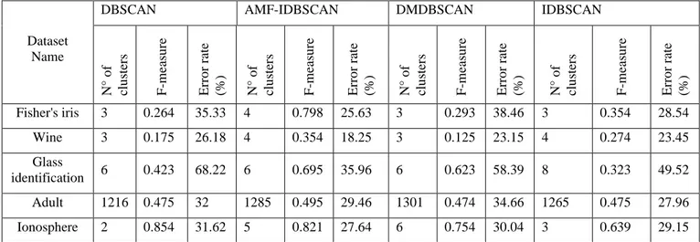
Table 6 compares the results obtained by our proposed algorithm against those of three other algorithms, namely: DBSCAN, IDBSCAN, and DMDBSCAN:
• From our experiments, and as Tables 2, 3, 4 and 5 show: by using the DBSCAN algorithm for multi-densities data sets, we get low-quality results with long times. DBSCAN algorithm is a time-consuming algorithm when dealing with large datasets. This is due to Eps and Minpts parameters values which are very important for DBSCAN algorithm, but their calculations are time-consuming. In other sense, clustering algorithms are in need to discover a better version of the DBSCAN algorithm to deal with these special multi-densities datasets.
• DMDBSCAN gives better efficiency results than DBSCAN clustering algorithm but takes more time compared with the other algorithms. This is due that the algorithm needs to call the DBSCAN algorithm for each value of Eps.
• The IDBSCAN algorithm is more efficient in terms of error rate and f-measure than DBSCAN algorithm. Also, it takes more time compared with DBSCAN, DMDBSCAN, and AMF-IDBSCAN. This is due to the fact that this algorithm needs to call the DBSCAN algorithm to make the initial clustering.
• AMF-IDBSCAN gives the best efficiency results compared to the other studiedalgorithms. Table 6 presents the F-Measure values recorded for all the data sets and all the algorithms. A high value of F-Measure proves the better quality of the clustering process. A significant improvement is found on AMF-IDBSCAN and on all datasets except the Ionosphere dataset. The maximum increase is observed in both Iris and Glass data sets. The improvement in F-Measure shows that our proposed method is more efficient in terms of
noise removal and outlier labeling. Apart from F-Measure, our proposed method allows to achieve good clustering results in a reasonable time. It can be easily observed from Figure 5 that our proposed clustering method for noise removal is well suited for high dimensional data sets and it exceeds the other existing methods.
5
Conclusion and perspectives
In this paper, we proposed AMF-IDBSCAN an enhanced version of the DBSCAN algorithm, including the notions of density, canopies and noise removal. This work presents a comparative study of the performance of this proposed approach which is fused with an adaptive median filtering median for noise removal and outlier detection technique and a canopy clustering method to reduce the volume of large datasets.
We compared this algorithm with the original DBSCAN algorithm, IDBSCAN, DMDBSCAN, and our experimental results show that the proposed approach gives better results in terms of error rate and f-measure with the increment of data in the original database.
In our future works, we will extend our investigations to other incremental clustering algorithms like COBWEB, incremental OPTICS and incremental supervised algorithms like incremental SVM, learn++, etc.
One of the remaining interesting challenges is how to select the algorithm parameters like k-dist, eps, Minpts, and number of canopies automatically.
6
Acknowledgment
The authors are grateful to the anonymous referees for their very constructive remarks and suggestions.
Figure 5: F-Measure (FM) Comparison across all Datasets.
7
References
[1] Patil Y.S., Vaidya M.B. (2012). A technical survey on cluster analysis in data mining. Journal of Emerging Technology and Advance Engineering, 2(9):503-513.
[2] ur Rehman S., Khan M.N.A. (2010). An incremental density-based clustering technique for large datasets. In Computational Intelligence in Security for Information Systems., Springer, Berlin, Heidelberg,pp. 3-11.
http:// doi.org/10.1007/978-3-642-16626-6_1 [3] Abudalfa S., Mikki M. (2013). K-means algorithm
with a novel distance measure. Turkish Journal of
Electrical Engineering & Computer
Sciences, 21(6): 1665-1684.
https://doi.org/10.3906/elk-1010-869.
[4] Kumar K. M., Reddy A. R. M. (2016). A fast DBSCAN clustering algorithm by accelerating neighbor searching using Groups method. Pattern Recognition, 58:39-48.
https://doi.org /10.1016/j.patcog.2016.03.008. [5] Kulkarni P. A., Mulay P. (2013). Evolve systems
using incremental clustering approach. Evolving Systems, 4(2): 71-85.
https://doi.org /10.1007/s12530-012-9068-z. [6] Goyal N., Goyal P., Venkatramaiah K., Deepak P.
C., Sanoop P. S. (2011, August). An efficient density based incremental clustering algorithm in data warehousing environment. In 2009 International Conference on Computer Engineering and Applications, IPCSIT , 2: 482-486.
https://doi.org/10.1016/j.aej.2015.08.009.
[7] Tseng F., Filev D., Chinnam R. B. (2017). A mutual information based online evolving clustering approach and its applications. Evolving Systems, 8(3): 179-191.
https://doi.org/10.1007/s12530-017-9191-y.
[8] Liu X., Yang Q., He L. (2017). A novel DBSCAN with entropy and probability for mixed data. Cluster Computing, 20(2):1313-1323.
https://doi.org/10.1007/s10586-017-0818-3.
[9] Suthar N., Indr P., Vinit P. (2013). A Technical Survey on DBSCAN Clustering Algorithm. Int. J. Sci. Eng. Res, 4:1775-1781.
[10] Ram A., Jalal S., Jalal A. S., Kumar M. (2010). DVBSCAN: A density based algorithm for discovering density varied clusters in large spatial databases. International Journal of Computer Applications, pp. 0975-8887.
https://doi.org/10.5120/739-1038.
[11] Birant D., Kut A. (2007). ST-DBSCAN: An algorithm for clustering spatial–temporal data. Data & Knowledge Engineering, 60(1): 208-221.
https://doi.org/10.1016/j.datak.2006.01.013. [12] Liu P., Zhou D., Wu N. (2007, June). Varied
density based spatial clustering of application with noise. In International Conference on Service Systems and Service Management, p. 21.
https://doi.org/10.1109/ICSSSM.2007.4280175. [13] Elbatta M. N. (2012). An improvement for
DBSCAN algorithm for best results in varied densities.
https://doi.org/10.1109/MITE.2013.6756302. [14] Elbatta M. T., Ashour W. M. (2013). A dynamic
method for discovering density varied clusters, 6(1). [15] Viswanath P., Pinkesh R. (2006, August). l-dbscan:
A fast hybrid density based clustering method.
In 18th International Conference on Pattern Recognition (ICPR'06), IEEE, 1: 912-915.
https://doi.org/10.1109/ICPR.2006.741.
https://doi.org/10.1109/ICSMC.2006.384571. [17] Liu B. (2006, August). A fast density-based
clustering algorithm for large databases. In 2006 International Conference on Machine Learning and Cybernetics IEEE,pp. 996-1000.
https://doi.org /10.1109/ICMLC.2006.258531. [18] He Y., Tan H., Luo W., Mao H., Ma D., Feng S.,
Fan J. (2011, December). Mr-dbscan: an efficient parallel density-based clustering algorithm using mapreduce. In 2011 IEEE 17th International Conference on Parallel and Distributed Systems, IEEE, pp. 473-480.
https://doi.org /10.1109/ICPADS.2011.83.
[19] [19] Wang S., Liu Y., Shen B. (2016, July). MDBSCAN: Multi-level density based spatial clustering of applications with noise.
In Proceedings of the 11th International Knowledge Management in Organizations Conference on The
changing face of Knowledge Management
Impacting Society, ACM, p. 21.
https://doi.org /10.1145/2925995.2926040.
[20] Swathi Kiruthika V., Thiagarasu Dr. V. (2017). FI-DBSCAN: Frequent Itemset Ultrametric Trees with Density Based Spatial Clustering Of Applications with Noise Using Mapreduce in Big Data.
International Journal of Innovative Research in Computer and Communication Engineering, 5: 56-64.
https://doi.org/ 10.15680/IJIRCCE.2017. 0501007 [21] Mai S. T., Assent I., Storgaard M. (2016, August).
AnyDBC: an efficient anytime density-based clustering algorithm for very large complex datasets. In Proceedings of the 22nd ACM SIGKDD international conference on knowledge discovery and data mining, ACM, pp. 1025-1034.
https://doi.org/ 10.1145/2939672.2939750.
[22] Bakr A. M., Ghanem N. M., Ismail M. A. (2015). Efficient incremental density-based algorithm for clustering large datasets. Alexandria Engineering Journal, 54(4):1147-1154.
https://doi.org/ 10.1016/j.aej.2015.08.009.
[23] Yada P., Sharma P. (2016). An Efficient Incremental Density based Clustering Algorithm Fused with Noise Removal and Outlier Labelling Technique. Indian Journal of Science and Technology, 9: 1-7.
https://doi.org/10.17485/ijst/2016/v9i48/106000. [24] McCallum A., Nigam K., Ungar L. H. (2000,
August). Efficient clustering of high-dimensional data sets with application to reference matching.
In Proceedings of the sixth ACM SIGKDD international conference on Knowledge discovery and data mining, ACM, pp. 169-178.
https://doi.org/10.1145/347090.347123.
[25] Kumar A., Ingle Y. S., Pande A., Dhule P. (2014). Canopy clustering: a review on pre-clustering approach to K-Means clustering. Int. J. Innov. Adv. Comput. Sci.(IJIACS), 3(5): 22-29.
[26] Ali T., Asghar S., Sajid N. A. (2010, June). Critical analysis of DBSCAN variations. In 2010
International Conference on Information and Emerging Technologies, IEEE, pp. 1-6.
https://doi.org/ 10.1109/ICIET.2010.5625720. [27] Ester M., Kriegel H. P., Sander J., Xu X. (1996,
August). A density-based algorithm for discovering clusters in large spatial databases with noise.
In Kdd, 96(34): 226-231.
[28] Moreira A., Santos M. Y., Carneiro S. (2005). Density-based clustering algorithms–DBSCAN and SNN. University of Minho-Portugal.
[29] Chakraborty S., Nagwani N. K. (2011). Analysis and study of Incremental DBSCAN clustering algorithm. International Journal of Enterprise Computing and Business Systems, 1: 101-130. https://doi.org/10.1007/978-3-642-22577-2_46. [30] Gu X., Angelov P. P., Kangin D., Principe J. C.
(2017). A new type of distance metric and its use for clustering. Evolving Systems, 8(3): 167-177. https://doi.org/10.1007/s12530-017-9195-7.
[31] Vijaykumar V. R., Jothibasu P. (2010, September). Decision based adaptive median filter to remove blotches, scratches, streaks, stripes and impulse noise in images. In 2010 IEEE International Conference on Image Processing, IEEE, pp. 117-120.
https://doi.org/10.1109/ICIP.2010.5651915. [32] Chen T., Wu H. R. (2001). Adaptive impulse
detection using center-weighted median filters. IEEE signal processing letters, 8(1): 1-3. https://doi.org/10.1109/97.889633.
[33] Zhao Y., Li D., Li Z. (2007, August). Performance enhancement and analysis of an adaptive median filter. In 2007 Second International Conference on Communications and Networking in China, IEEE,
pp. 651-653.
https://doi.org/10.1109/CHINACOM.2007.4469475 [34] Sasaki Y. (2007). The truth of the F-
measure. Teach Tutor mater, 1(5): 1-5. https://doi.org/10.13140/RG.2.1.1571.5369.