Model of Traffic Speed Flow Relationship at Signal Intersections

ISSN Online: 2165-3925 ISSN Print: 2165-3917

Model of Traffic Speed-Flow Relationship at

Signal Intersections

Yixin Chen

School of Transportation Engineering, Tongji University, Shanghai, China

Abstract

Speed-flow relationship is the fundamental for the traffic simulation and traf-fic volume forecast. Traditional quadratic polynomial model can’t reflect the saturate flow at signal intersections. In order to determine the speed-flow re-lationship at signal intersections, the speed and time-headway of vehicles at two signal intersections were investigated and the accuracy of software used to get the speed was tested. After vehicle starting-up from queuing, the time- headway reduces gradually with the increase of speed. The relationship of power exponential function between speed and time-headway is formulated. Traffic volume can be calculated by the vehicle time-headway. Then the speed-flow relationship was developed and an S-shaped curve model was built in this paper. In the S-shaped curve model, traffic flow approaches to the sa-turate when the speed doesn’t increase. Thus, S-shaped curve model is better to describe the speed-flow relationship at signal intersection. The results can provide a reference to determine the parameters in traffic simulation and for the study of level of service of intersections.

Keywords

Signal Intersections, Speed-Flow, Time-Headway, Power Exponential Function

1. Introduction

The relationship between speed and volume is the fundamental in the traffic flow theory. It was first studied by Greenshields. Then, there were many efforts to develop theoretical models, including models by Greenberg (1959), Under-wood (1961), and other models [1]. The Greenshields model is widely used, which is a quadratic polynomial model:

(

)

j f

Q=K V−V V (1)

Q: traffic flow rate;

How to cite this paper: Chen, Y.X. (2017) Model of Traffic Speed-Flow Relationship

at Signal Intersections. Open Journal of

Applied Sciences, 7, 319-327.

https://doi.org/10.4236/ojapps.2017.76025

Received: May 24, 2017 Accepted: June 26, 2017 Published: June 29, 2017

Copyright © 2017 by author and Scientific Research Publishing Inc. This work is licensed under the Creative Commons Attribution International License (CC BY 4.0).

Kj: critical density;

V: operating speed; Vj: free flow speed.

According to the ways of data collection and data analysis, there are many other different models, because of different. Guo, et al. [2] found that the traffic flow characteristics in expressway of Beijing were similar to those of highways in other countries. Based on the field data of urban streets, an adapted S-curve model was developed by Chen [3]. Shao analyzed the vehicles operation charac-ters on urban individual freeway lanes, and established a power exponential function model for the speed-flow relationship. At the same time, he pointed out that the speed decreased when traffic flow reaches a certain value [4]. Traffic flow was divided into three categories by Li [5]: free flow segment, stable flow segment, and congested-evacuation segment. Three models for the for the speed-flow relationship were built.

In summary, all the researches on the speed-flow relationship in China focus on the expressway. The speed (V) is the average operating speed, which con-taining all vehicles on investigated section of the road. This can not apply for the intersections. After starting-up for the queuing vehicles, the time-headway re-duces gradually as the speed increases and the flow rate ends up with the satura-tion rate. This is different from the characters of traffic flow on highways and freeways. At the same time, the actual models were quadratic polynomial model, exponential or logarithmic function model. These models can’t reflect the satu-rate flow at signal intersections.

The purpose of this paper is to develop the model of speed-flow relationship at signal intersection. After vehicle starting-up from queuing, the time-headway reduces gradually with the increase of speed. The speed and time-headway of vehicles at signal intersections were investigated and the relationship between them was formulated. Traffic volume can be calculated by the vehicle time- headway. Then the speed-flow relationship can be developed.

2. Data Collection

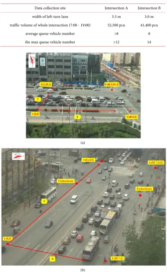
The imagery data have been collected by a camera placed at corners of two in-tersections in order to get the accurate bird-view. These typical urban four- ap-proach intersections operate with a four-phase signal plan with a protected left-turn phase for both heavily traveled streets. The data collection lasts for three consecutive workdays for each signal intersections. The data are collected under good weather with only small vehicles (excluding the data from the pro-tected phase when buses, large trucks and U-turn vehicles are present). The in-formation for the investigated intersections is shown in Table 1.

the intersections (Figure 1).

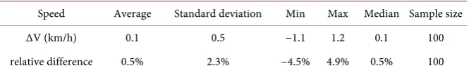
The accuracy for the measurement error of speed gotten by the software is tested, which is shown in Figure 2. Two lines are painted on the ground (l1, l2),

and the distance between them is two meters (L12). Then the actual travel speed

(V1) can be calculated. The difference between the actual travel speed (V1) and Table 1. Information of the investigated intersections.

Data collection site Intersection A Intersection B

width of left-turn lane 3.3 m 3.0 m

traffic volume of whole intersection (7:00 - 19:00) 52,500 pcu 41,400 pcu

average queue vehicle number >8 8

the max queue vehicle number >12 14

(a)

(b)

Figure 2. Accuracy test for the measurement error of speed.

Table 2. Measurement test of speed.

Speed Average Standard deviation Min Max Median Sample size

∆V (km/h) 0.1 0.5 −1.1 1.2 0.1 100

relative difference 0.5% 2.3% −4.5% 4.9% 0.5% 100

the travel speed (V2) obtained by the positioning software is the measurement

error.

The results of accuracy test are illustrated in Table 2. The average difference between V1 and V2 is 0.1 km/h, and the max is ±1.2 km/h, the relative difference

of the speed is within 5%. Thus, the vehicle speed got from the software can be used to build the model of speed-flow Relationship.

3. Analysis

Assume that the first vehicle in the queue starts from the stop line, and the initial velocity is zero. Vehicles followed the front one. The time-headway of vehicles (Ht) can be expressed as:

t 2 1

H =T −T (2)

where,

Ht = time-headway of vehicle(s); 2

T = the time when the front car passes through the stop line;

T1 = the time when the following car passes through the stop line.

The vehicle speed (V) is the average speed between the front vehicle passes through the stop line and the vehicle itself passes through. It can be calculated as follows.

( )

( )

2

V T V T

V = + (3)

where,

( )

V T = the speed of the following car when the front car passes through the

stop line;

( )

V T = the speed of the following car when it passes through the stop line. 3.1. Model of Time-Headway and Speed (Ht-V)

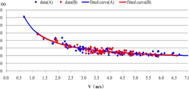
According to the investigated data, the scatter plots of time-headway and speed were displayed in Figure 3. The time-headway (Ht) reduced gradually as the speed (V) increased and the flow rate ended up with the saturation rate from zero. The speed of saturation flow at intersection A was 6.5 m/s, and 5.5 m/s at intersection B. The time-headway of saturation flow is about two seconds.

Vehicles started one by one from queuing. The start-up reaction time for dif-ferent drivers is approximate [6]. Then, the following conclusions can be found so far: 1) time-headway (Ht) reduces gradually as the speed increases; 2) time-

headway (Ht) is greater than a certain value. Thus, the power exponential

func-tion is selected to fit the relafunc-tionship between Ht and V, which is showed in

Equ-ation (4).

t

b

H = ×a V +c (4)

where:

Ht = time-headway of vehicle (s);

V = speed (m/s);

a, b, c: constant parameter.

The equations fitted by the field data using the software at intersection A, B are as follows:

( )

A 4.42 1.13 t

H = ×V− + (5)

( )

B 4.57 1.06 t

H = ×V− + (6)

Ht(A): time-headway of vehicle at intersection A (s);

Ht(B): time-headway of vehicle at intersection B (s).

The correlation coefficient (R-square) is 0.89 at intersection A and 0.81 at in-tersection B.

3.2. Model Checking

The Ht of saturate flow is the minimum at signal intersection. At this time, Ht

can be expressed as flow:

d f r d

ts r

f f

h V t h

H t

V V

+ ×

= = + ₍₇₎

where:

Hts = time-headway of saturate flow (s);

hd = distance-headway of the queuing vehicles(m);

Vf: speed of saturate flow (m/s);

tr: start-up reaction time for queuing vehicles(s).

When Vf →∞，the Hts→tr (Equation (7)), tr is the reaction times of the

queuing vehicles, which is the constant parameter c in Equation (4). According to the Equations ((5) and (6)), the average reaction time is 1.13 s at intersection A, and 1.06 s at intersection B.

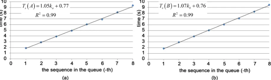
The reaction time also can be investigated by the field video. The queuing ve-hicles begin to start one by one after the start-up reaction and the lag of start-up time between adjacent queuing vehicles is the reaction time. A linear regression model [6] is used to describe the law of start-up time (Figure 4, (Equations ((8), (9))). The results showed that reaction time at intersection A is 1.05 s and 1.07 s at intersection B.

The fitting formulas are as follows: Intersection A:

( )

s 1.05 a 0.77

T A = ×K + (8)

Intersection B:

( )

s 1.07 b 0.76

T B = ×K + (9)

Ts: the start-time after the green light(s);

Ka: queue order (intersection A);

Kb: queue order (intersection B).

The two reaction times (model of time-headway in Equations ((5), (6)) and investigated by the field video) were compared in Table 3. Two of them were approximate. Thus, the model of time-headway is reasonable.

Table 3. Comparison to the Tr(reaction time).

Tr (reaction time) Calculate by fitted equation Actual Relative difference

A 1.13 1.05 7.1%

B 1.06 1.07 0.9%

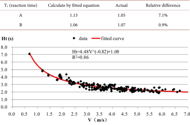
Figure 5. Fitted model for the Ht-V relationship.

3.3. Speed-Flow Relationship

The final power exponential function of Ht-V is fitted by the combined data

(in-tersection A and in(in-tersection B), which is showed in Figure 5.

The relationship between traffic flow rate (Q) and time-headway (Ht) is as

follows:

3600 3600

b t

Q

H a V c

= =

× + (10)

Q: traffic flow rate (pcu/h); Thus, Speed-Flow Relationship is:

0.82

3600 3600

4.48 1.08

t

Q

H V−

= =

× + (11)

Equation (11) is a formula of S-shaped curve. In the speed-flow relationship, the Q increases gradually with the speed increases after vehicle starting-up. Traf-fic flow approaches to the saturation when the speed (V) doesn’t increase. The constant parameters a and c are greater than zero, and b is smaller than zero but greater than negative one. The value c represents the reaction time of drivers.

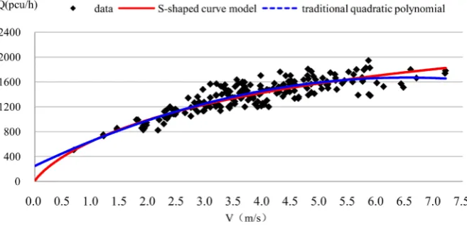
Figure 6. Comparison of two models.

When speed is zero, the traffic flow rate (Q) is also zero.

The S-shaped curve model developed in this paper is well to fit the speed-flow relationship, and it can reflect the character of stable saturate flow. Thus, the V-flow relationship of S-shaped curve model is better than traditional quadratic polynomial model at signal intersections.

4. Conclusions

In order to explore the speed-flow relationship at signal intersections, the im-agery data have been collected by a camera placed at two intersections. The rela-tionship between speed and time-headway is analyzed and a law of power expo-nential function is formulated in this paper. Based on the field data, the equation is fitted by the software and it is tested by the parameter of reaction time of the drivers. Then, the model of speed-flow relationship (S-shaped curve) is devel-oped.

After vehicle starting-up from queuing, the time-headway reduces gradually with the increase of speed and traffic flow approaches to the saturate when the speed (V) doesn’t increase. The S-shaped curve model developed in this paper can reflect these characters. Through analyzing the traffic data, the error of tra-ditional quadratic polynomial model will be larger as the flow reaches to satura-tion and the speed further increases. Thus, the S-shaped curve model is better to fit the speed-flow relationship at signal intersections.

Acknowledgements

This study was sponsored by the Open Project of Key Laboratory of Ministry of Public Security for Road Traffic Safety (2016ZDSYSKFKT06).

References

[1] Xu, J.Q. and Chen, X.W. (2008) Fundamentals of Traffic Engineer. 3rd Edition, China Communications Press, Beijing.

[2] Guo, J.F., Qua, Y.S., Zheng, M. and Li, X. (2002) Study on the Traffic Flow of the Expressway System in Bejing. Urban Transport, 24, 42-44.

Ph.D. Thesis, Southeast University, Nanjing.

[4] Shao, C.Q. and Zhao, L. (2006) Study of Speed-Flow Relationships Model on Urban Individual Freeway Lanes. Road Traffic and Safety, 6, 8-10.

[5] Li,Y., Lu, H.P., Bian, C.Z. and Sui, Y. (2009) Traffic Speed-Flow Model for the Mix Traffic Flow on Beijing Urban Expressway. International Conference on Measuring Technology and Mechatronics Automation (ICMTMA), 3, 641-644.

https://doi.org/10.1109/ICMTMA.2009.312

[6] Zong, E. (2007) Research on Capacity of Left-Turn Lanes at Signalized Intersection. Master’s Thesis, Beijing University of Technology, Beijing.

Submit or recommend next manuscript to SCIRP and we will provide best service for you:

Accepting pre-submission inquiries through Email, Facebook, LinkedIn, Twitter, etc. A wide selection of journals (inclusive of 9 subjects, more than 200 journals)

Providing 24-hour high-quality service User-friendly online submission system Fair and swift peer-review system

Efficient typesetting and proofreading procedure

Display of the result of downloads and visits, as well as the number of cited articles Maximum dissemination of your research work

Submit your manuscript at: http://papersubmission.scirp.org/