Forecasting Economic Aggregates Using Dynamic Component Grouping

Munich Personal RePEc Archive

Forecasting Economic Aggregates Using

Dynamic Component Grouping

Cobb, Marcus P A

September 2017

Online at

https://mpra.ub.uni-muenchen.de/81585/

Forecasting Economic Aggregates Using Dynamic

Component Grouping

Marcus P. A. Cobb

∗

September 2017

Abstract

In terms of aggregate accuracy, whether it is worth the effort of modelling a dis-aggregate process, instead of forecasting the dis-aggregate directly, depends on the properties of the data. Forecasting the aggregate directly and forecasting each of the components separately, however, are not the only options. This paper develops a framework to forecast an aggregate that dynamically chooses groupings of com-ponents based on the properties of the data to benefit from both the advantages of aggregation and disaggregation. With this objective in mind, the dimension of the problem is reduced by selecting a subset of possible groupings through the use of agglomerative hierarchical clustering. The definitive forecast is then produced based on this subset. The results from an empirical application using CPI data for France, Germany and the UK suggest that the grouping methods can improve both aggregate and disaggregate accuracy.

Keywords: Forecasting economic aggregates; Bottom-up forecasting; Hierarchical forecasting; Hierarchical Clustering;

JEL codes: C38, C53, E37

Non-technical Summary

When forecasting economic aggregates, practitioners are faced with many options even when only the level of disaggregation is considered. These include forecasting at the level of disaggregation that is required to answer a particular question, disaggregat-ing further or forecastdisaggregat-ing at a more aggregate level and reconcildisaggregat-ing the lower levels of disaggregation if necessary. The usual argument behind using the components is that allowing for different specifications across disaggregate variables may capture more precisely the dynamics of a process that becomes too complex through aggregation. Favouring forecasting directly is that it would be less affected by disaggregate mis-specification, data measurement error and structural breaks. Ultimately, whether it is better to forecast components together or separately depends on the particular fore-casting models and data. An option to improve forefore-casting performance in this setting, is to work on the modelling and another is to look for data transformations that allow existing models to perform better. This paper presents a framework to do the latter.

Grouping components together can produce new series with characteristics that differ quite significantly from those of the originating series. In this context, it might be possible to find specific groupings that avoid the problems associated with disaggregate forecasting while still allowing for distinct disaggregate dynamics to be picked up in the process. With this objective we develop a two-stage method that combines statistical learning techniques and traditional economic forecasting evaluation. In the first stage, we use agglomerative hierarchical clustering to reduce the dimension of the problem by choosing a subset of feasible groupings based on the commonality among the different components. In the second stage, we try different selection procedures on the resulting hierarchy to produce the final aggregate forecast. These selection procedures include choosing a single grouping based on some criterion and combining the whole subset of groups.

1

Introduction

When forecasting economic aggregates, practitioners are often faced with the choice of either forecasting them directly or forecasting their components and then summing them up. Sometimes the choice may be influenced by considerations other than accur-acy, like when a questions cannot be answered just by looking at the aggregate or an underlying scenario for the aggregate forecast is needed. Nevertheless, even in these cases, aggregate forecasting accuracy is usually a concern (Esteves, 2013).

The options available for forecasting are many, even when only the level of disaggreg-ation is considered. These include forecasting at the level of disaggregdisaggreg-ation that is required to answer a particular question, disaggregating further or forecasting at a more aggregate level and reconciling the lower levels of disaggregation if necessary.

The usual argument behind using the components to forecast an aggregate is that al-lowing for different specifications across disaggregate variables may capture more pre-cisely the dynamics of a process that becomes too complex through aggregation (Barker and Pesaran, 1990). In support of this view, Granger (1990) show that the summing many simple stationary processes can produce a fractional integrated aggregate, while Bermingham and D’Agostino (2014) show that the dispersion of the persistence of indi-vidual series has an accelerating effect on the increase of complexity in the aggregate.

Favouring forecasting the aggregate directly is that, in practical applications, it is likely that the disaggregate processes may suffer from misspecification. For example, if the disaggregate models neglect that a number of components share common factors, the forecasting errors will tend to cluster having a negative effect on the aggregate forecast (Granger, 1987). The direct aggregate forecast would be less affected by these features in the data and other problems, like those resulting from data measurement error and structural breaks (Grunfeld and Griliches, 1960; Aigner and Goldfeld, 1974).

The theoretical literature supports using the disaggregate forecasts, or bottom-up ap-proach, but the results in the empirical literature are mixed.1 Ultimately, whether the magnitude of the aggregation error compensates the specification errors in the disag-gregate model depends on the particular forecasting models and data (Pesaran et al., 1989).

An option to improve forecasting performance in this setting, is to work on the model-ling, like Hendry and Hubrich (2011) that include disaggregate information in a direct

1

aggregate approach or Bermingham and D’Agostino (2014) that include common factors in a bottom-up approach. Another less obvious way, is to look for data transformations that allow existing models to perform better.

As mentioned before, adding components together results in new series with charac-teristics that may differ quite significantly from those of the originating ones. In this context, it may be possible to purposefully find specific groupings that show more de-sirable properties than those of the individual components and the aggregate.

Some authors have proposed using purpose-built groupings to increase overall fore-casting accuracy, but it would seem that, at least in economic forefore-casting, it has had little impact (Duncan et al., 2001). A reason for this may be that the number of possible groupings grows exponentially with the number of components meaning that traditional methods, that would usually rely on evaluating all possible outcomes, are really only us-able for problems with relatively few components.2 For larger problems, a different approach becomes necessary.

One that has been relatively successful recently, particularly given the increase in pop-ularity of methods for Big Data, is one that performs grouping conditional on some fea-ture of the original data. These have been in use for a while in the context of electricity price forecasting (Weron, 2014) and, with the relatively recent surge in computational power, computer intensive methods and availability of high-frequency data, they have expanded to other areas of research. For example, Yan et al. (2013) report significant improvements in the context of wind power prediction, Jha et al. (2015) for inventory planning in retail and Gao and Yang (2014) for forecasting stock market returns.

The success of these methods, however, depends on the chosen feature being useful in obtaining the desired outcome. The assumption upon which many of these models are built on, is that by grouping series that behave in a similar way, the idiosyncratic errors within groups will tend to offset each other while the more relevant individual dynamics will be retained to be modelled.

Although these problems are set in a different context, the purpose of the methods are very similar to those of grouping components to increase the forecasting accuracy of an economic aggregate. They belong, however, to an area of research of statistical learning that has focused almost exclusively on extracting information from very large datasets. Many relevant economic aggregates, like GDP and CPI, do not fall in this category and it is unclear whether these methods will work with relatively small samples.

2

In this context, we develop a method to forecast economic aggregates based on pur-pose built groupings of components using statistical learning techniques. The two-stage method consists of trying to find the grouping of components at each point in time that produces the best aggregate forecast. In the first stage, we use agglomerative hier-archical clustering to reduce the dimension of the problem and, in the second, we use a selection procedure on the resulting hierarchy to produce the final aggregate forecast.

The rest of the paper is organized as follows. Section 2 presents the component group-ing framework. Section 3 presents an empirical implementation usgroup-ing CPI data for France, Germany and the United Kingdom. Section 4 summarizes the conclusions.

2

A purpose driven grouping framework for aggregate

fore-casting

As pointed out by James et al. (2013), Statistical Learning refers to a broad set of tools for understanding data. These include some approaches that are intended for prediction among other objectives. They usually require computing the input and output for each event which may be undesirable in problems that are very large. Other methods try to learn relationships and structure from a dataset without a clear objective. They work directly and produce results based on the features of the original data and require, therefore, significantly less computation. The challenge of using these methods lies in tuning the algorithms so that they achieve a desired purpose.

Although the implementations and techniques differ, the assumption on which many of the models intended to forecast time-series are built on, is that forecasting series that behave similarly as a group will tend to produce more accurate aggregate forecasts than if they are modelled separately. This assumption would also seem reasonable within the context of forecasting economic aggregates, given that the relevant literature shows that accounting for commonality among components is key to forecasting accuracy and, in particular, that ignoring it would be detrimental for the bottom-up approach (Duarte and Rua, 2007; Espasa and Mayo-Burgos, 2013; Bermingham and D’Agostino, 2014).3

Regarding the method that performs the grouping, within the area of unsupervised learning there are many.4 One that seems well suited for the particular setting is Hier-archical Clustering. The method is concerned with discovering unknown subgroups in

3_{This view goes beyond the direct versus bottom-up debate. The success of the dynamic factor models,} proposed initially by Geweke (1977) and extended by Stock and Watson (2002) and Forni et al. (2005) among others, is just an example.

4

data. The most commonly used method is the agglomerative alternative, that starts with a set of groups, or clusters, that contain a single element each and proceeds by group-ing the data into fewer units with more elements each.5 The only thing the algorithm needs to work is some sort of dissimilarity measure between each pair of observations and then one for each cluster that is formed. For the fused clusters, those other than those containing a single original observation, typically the dissimilarity measures are calculated from the original dissimilarity measures following a procedure referred to as linkage. The result of running the algorithm is always a hierarchical structure that has exactly as many levels as the number of initial components, with the individual compon-ents as the lowest level and the aggregate as the highest. In the context of grouping for forecasting, this means that the direct aggregate and bottom-up approaches are always available as options to be chosen to produce the definitive forecast.

At first sight, it could seem that hierarchical clustering might be the solution to the grouping problem. However, the method provides no guidance on whether the group-ings in the structure are meaningful nor if one grouping is better than another in any particular sense (Murphy, 2012).6 _{This could be seen as a drawback, but, in the context}

of forecasting the economic aggregate, it might work out as an advantage.

The problem with identifying an appropriate grouping right away, is that, even if there is one, the particular dissimilarity threshold below which components should be grouped so as to obtain the most accurate aggregate forecast is unknown. By narrowing down the set of groupings, however, the clustering process reduces the initial problem to a manageable size that can then be tackled with evaluation methods that are common in the traditional forecasting literature.

In what follows, we present a two-stage grouping framework to forecast economic ag-gregates, that consists of defining the hierarchy, based on the commonality among com-ponents, and then choosing how to produce the definitive aggregate forecast based on that hierarchy.

2.1

Guided selection of a subset of groupings

Dissimilarity measures and linkage methods have a defining impact on the results and the relevant literature provides many alternatives to choose from. As James et al. (2013) point out, the choice of what alternative to use depends on the type of data and question at hand.

5

The less popular divisive approach starts from one large group that contains all the elements and divides it up accordingly.

6

In the statistical learning literature it is not unusual to use simple correlation as the dis-similarity measure for time-series. The forecasting literature, however, points towards the notion of commonality. The problem is that there is not a unique way of measure it. For this reason we present six different possibilities based on what has been suggested in the literature.

All but one of the measures are used within the context of the traditional hierarchical clustering approach that is deterministic. The exception is set within a probabilistic framework. In nature they are very similar given that both have a hierarchy as the outcome. The fundamental difference is that the more common deterministic method needs to be provided with dissimilarity measures. The probabilistic method, on the other hand, works out the dissimilarity from the data itself. It therefore makes sense to present them separately.

2.1.1 Deterministic grouping algorithm

The implementations of deterministic agglomerative hierarchical clustering are relat-ively simple.7 In the context of an aggregate with

n

components, the algorithm proceeds by calculating the pairwise commonality between the

n

series and aggregating the two with the highest commonality. This leaves

n

−

1

series. The traditional approach would involve calculating the pairwise commonality of the new cluster with the remaining com-ponents using a particular linkage method and proceed to aggregate the next two series with the highest commonality. The process is repeated until only the aggregate is left.

In a departure from the standard clustering algorithm, for our implementation, at each step, we calculate the pairwise commonality between the newly formed cluster and the remaining components by computing the dissimilarity measures between the new series instead of using linkage.8 This makes the approach slower, but, by not using a linkage method, it does not make any assumptions regarding how the commonality transmits from the components to the aggregate.

For the dissimilarity measures, five measures are evaluated:

Pearson’s Correlation

In the machine learning literature there are many alternatives, but in the context of time-series the most obvious are measures for correlation. Probably the best known is Pearson’s correlation coefficient that measures the strength of the linear relationship

7_{Detailed descriptions may be found in standard Statistical Learning texts and surveys like Hastie et al.} (2009), Murtagh and Contreras (2012) or James et al. (2013).

between two variables. Although its limitations are many, its widespread use make it an obvious benchmark for the rest of the measures.

The correlation coefficient between

x

i and

x

j is defined as

ρ

xixj

=

cov(xi,xj)

σ_xiσ_xj , where

cov

(

x

i

, x

j

)

is the covariance between

x

i and

x

j and

σ

xi,σxj are the respective

stand-ard deviations. As a higher correlation, in absolute terms, is associated with similarity, the corresponding dissimilarity measure is defined as:

P C

xi,xj

= 1

−

abs

cov

(

x

i

, x

j

)

σ

xi

σ

xj

Spearman’s Correlation

As pointed out by Hauke and Kossowski (2011), sometimes the Pearson’s correlation coefficient can produce results that are undesirable or misleading. This can be a result of being restricted to linearity or requiring variables to be measured on interval scales.

Spearman’s rank correlation coefficient is a non-parametric rank statistic that assesses how well an arbitrary monotonic function can describe the relationship between two variables. Therefore, it is not affected by non-linearity. In practice, however, it is just the Pearson’s Correlation coefficient in which the data are converted to ranks before calculating the coefficient.

The rank correlation coefficient between

x

i and

x

j is defined as

r

xixj

=

cov(xrank i ,xrankj )

σ_xrank

i

σ_xrank

j

,

where

x

rank

i and

x

rankj are the ranks of

x

i and

x

j respectively. Again, as a higher

cor-relation, in absolute terms, is associated with similarity, the corresponding dissimilarity measure is defined as:

SC

xi,xj

= 1

−

abs

cov

(

x

rank

i

, x

rankj

)

σ

_xrank i

σ

xrankj

!

Latent factor

As explained by Hastie et al. (2009), for

n

series of length

T

, the sample’s covariance matrix _T1

X

T

X

can be rewritten using the eigen decomposition as

VD

2

V

T

. The columns of

V, the eigenvectors, are the principal component directions of

X

and

z

1

=

Xv

1, with

v

1 being the first column of

V, is the first principal component. The values on the

diagonal of

D

2

are the eigenvalues associated with each eigenvector, that is

d

2₁ for

v

1.

It can be shown that

Var(

z

1

) = Var(

Xv

1

) =

d

2 1

T. Then, the total variance explained by the

first principal component isd2

1

/

Pnl=1d2l. As a higher total explained variance is associated

with similarity, the corresponding dissimilarity measure is defined as:

V E

xi,xj

= 1

−

d

2₁

P

n l=1

d

2l

Persistence

Bermingham and D’Agostino (2014) point out that series that have very different per-sistence will tend to suffer more of omitted variable bias if they are forecasted together than series with a similar persistence. They advocate forecasting series with different persistence separately.

To take up this point, we fit an AR(1) model to each component,

x

i,t

=

a

i

+

ρ

i

x

i,t−1

+

ǫ

i,t, and use the difference in the estimated persistence parameter as a measure for

dissimilarity:

P E

xi,xj

= abs (abs (ˆ

ρ

i

)

−

abs (ˆ

ρ

j

))

Forecast-error clustering

Bermingham and D’Agostino (2014) also state that ignoring the common factor and interdependencies will tend to make forecasting errors cluster instead of cancelling out.

Having this phenomenon in mind, we again fit AR(1) models to each component but this time we use as the dissimilarity measure the correlations of the out-of-sample forecast-ing errors for the most recent periods.

Specifically, for each component

i

we fit

x

i,t−p+1

=

a

i

+

ρx

i,t−p

+

ǫ

i,t, where

p

is the number

of periods that are evaluated for the measure. With the model, we generate forecasts from

t

−

p

+ 1

to

t

and calculate the corresponding forecasting errors as

x

ˆ

i,s|s-1

−

x

i,s for

s

=

t

−

p

+ 1

to

t

and collect them in

ˆ

e

t_i. With this, the dissimilarity measure is defined as:

F C

xi,xj

= 1

−

abs

cov

(ˆ

e

t_i

,

e

ˆ

t_j

)

σ

_ˆet

2.1.2 Probabilistic grouping algorithm

As pointed out by Murphy (2012), it would be desirable for a clustering method to provide some insight into the quality of the groupings. However, as traditional clus-tering methods are deterministic, this is not possible. Probabilistic algorithms have been proposed, but until recently their increased complexity have hindered their imple-mentation.

One that does compare favourably to the traditional methods is the Bayesian Hier-archical Clustering method by Heller and Ghahramani (2005). The main idea, is that, through empirical Bayesian methods, it performs the grouping based on the probability of two observations being generated from the same underlying function.

The essence of the method can be seen from the explanation in Murphy (2012).9 Let

D

=

{

x

1

, . . . , x

n

}

represent all the data and

D

i the data at subtree

T

i. Then, at each

step, subtrees

T

i and

T

j are compared to see if they should be merged together. The

hypothesis to be evaluated, is that

x

i and

x

j come from the same probabilistic model

p

(

x

|

θ

)

of unknown parameters

θ. Then define

D

ij as the merged data, and let

M

ij

equal one if they should be merged and zero if they should not. The probability of a merge is given by

r

ij

=

p

(

D

ij

|

M

ij

= 1)

p

(

M

ij

= 1)

p

(

D

ij

|

M

ij

= 1)

p

(

M

ij

= 1) +

p

(

D

ij

|

M

ij

= 0)

p

(

M

ij

= 0)

p

(

M

ij

= 1)

is the prior probability of a merge and can be computed from the data (Heller

and Ghahramani, 2005). If

M

ij equal to one, the data is assumed to come from the same

model meaning

p

(

D

ij

|

M

ij

= 1) =

Z





Y

xn∈Dij

p

(

x

n

|

θ

)





p

(

θ

|

λ

)

dθ

with

λ

being a hyperparameter than can be provided or estimated from the data. If

M

ij

equal to zero, the data is assumed to generated independently and

p

(

D

ij

|

M

ij

= 0) =

p

(

D

i

|

T

i

)

p

(

D

j

|

T

j

)

With this, all the elements to build the hierarchy are available.

The algorithm starts with each observation in its own cluster. It calculates all the pair-wise merge probabilities and proceeds to merge the clusters with the highest posterior merge probability. It then recalculates the pairwise merge probabilities. It continues in

this way, merging the pairs with the highest merge probability until only the aggregate is left.

The method is developed for cross-section, but Cooke et al. (2011) extend it to time-series in the context of gene expression measurement. Through the introduction of Gaussian process regression, an equivalent grouping process is performed based on the probability of two observations having the same latent function.

2.2

Producing a unique aggregate forecast

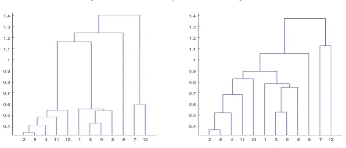
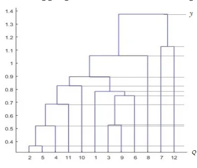
The outcome from the clustering algorithm is a complete hierarchy and because of the way the algorithm works it will offer a number of levels of aggregation equal to the number of original components. As the hierarchical clustering proceeds by fusing two observations or series at a time, it produces an intuitive tree-based representation of the final structure. This representation is called a dendrogram. Figure 1 shows two dif-ferent examples for twelve components. At the bottom are all the individual elements. Moving up some of the elements are paired with similar observations producing a num-ber of clusters. Higher up, the clusters themselves fuse, either with single elements or other clusters.

As mentioned before, the algorithm by itself does not provide any advice with regards to what grouping to use.10 On the dendrogram, however, the vertical axis presents the level of dissimilarity and therefore visual inspection can provide some guidance.

Choosing a grouping based on some specific dissimilarity level is equivalent to drawing a horizontal line across the dendrogram at that desired level and using the groupings that are formed below that line. In Figure 1, for example, the dendrogram on the left suggests that there are four distinct groups based on the distance between the fusions. This, because the four groups form relatively close to the bottom and are only fused again relatively near to the top. More often than not, however, visual inspection is not enough to learn appropriate groupings (Murphy, 2012; James et al., 2013). That is, it is not uncommon that no obvious cutting points are revealed. The hierarchy depicted on the right of Figure 1, serves as an example. In these cases it is necessary turn to an exogenous criterion.

For this purpose, we present six different alternatives separating the methods in those that seek to select a single level of disaggregation and those that use a combination of the different groupings.

[image:13.595.123.470.118.266.2]

Figure 1: An example of dendrograms

2.2.1 Disaggregation level selection

In-sample fit

Probably the most commonly used approach to judge a model is in-sample fit. It has some known drawbacks, but its widespread use makes it a natural choice. For our par-ticular case we use the in-sample forecasting error. To choose the level of aggregation for forecasting period

t

+ 1

, for each level of aggregation within the proposed hierarchy at time

t, we use the forecasting models and parameters calculated using data up to

period

t

to calculate the one-step-ahead root mean squared forecasting error (RMSFE) for the sample up to period

t.

With this, the in-sample fit for disaggregation level

i, at time

t

is:

ISF

i,t,v

=

v

u

u

t

1

v

t−1

X

s=t−1−v

ˆ

x

i,s+1|t

−

x

i,s+1

2

where

v

determines how much data is included in the measure.

The level of aggregation with the lowest in-sample forecasting error is then used to forecast period

t

+ 1

.

Past out-of-sample forecasting performance

t

−

v

+ 2

and continue in the same way stopping with the forecast for period

t. Then, we

calculate the RMSFE using these forecasts.

With this, the out-of-sample performance for disaggregation level

i, at time

t

is:

OOS

i,t,v

=

v

u

u

t

1

v

t−1

X

s=t−1−v

ˆ

x

i,s+1|s

−

x

i,s+1

2

where

v

determines how much data is included in the measure.

The level of aggregation with the lowest out-of-sample forecasting error is then used to forecast period

t

+ 1

.

Lowest average error dissimilarity threshold

Unsupervised learning, of which the clustering method used to produce the subset of groups is part of, is often challenging because there is no response variable. In our context, however, the ultimate objective is to find the level of aggregation at which the resulting aggregate forecast error is lowest. For this purpose, we can use a supervised method to try to learn the best grouping for the purpose of forecasting. We do this by relating the degree of commonality, as measured by the corresponding dissimilarity measure, with the forecasting error.

The way in which we do this is by calculating for the training sample the average fore-casting error conditional on the level of dissimilarity. This corresponds to calculating the forecasting error associated with the values on the vertical axis of all the dendro-grams for the sample up to period

t

and averaging the results.11 To make the averaging over different periods possible, we use a smoothing spline to interpolate the forecast-ing errors for each period. To forecast period

t

+ 1

we choose the level of aggregation associated with the dissimilarity that is closest to the minimum average error.

Probabilistic criterion

The Bayesian Hierarchical Clustering method proceeds by building the hierarchy based on the estimated probability of two observations coming from the same underlying func-tion. Heller and Ghahramani (2005) suggest that a natural decision rule for groupings in this context, is to only perform fusions that have a posterior merge probability greater than 50%. This criterion, however, can only be applied to hierarchies produced by the probabilistic algorithm.

11

2.2.2 Disaggregation level averaging

A popular way of dealing with choosing between two or more competing forecasts is to avoid the decision all together and combine them. The idea of forecast combination has been around for a long time and deals with the issue of exploiting in the best pos-sible way the information contained in each individual forecasts. The literature on it is extensive and the surveys by Clemen (1989), Diebold and Lopez (1996), Newbold and Harvey (2002) and Timmermann (2006) not only give testimony of it but also highlight the robustness of the gains in forecasting accuracy due to its use.

Equal-weights among aggregate forecasts

A very attractive feature of forecast combination is that simple combination schemes are surprisingly effective (Timmermann, 2006). In fact, the equal-weighted forecast combination performs so well that researchers have tried to explain why this is the case (Smith and Wallis, 2009). In view of this, given that each level of the hierarchy produces an aggregate forecast, the most straightforward thing is to average the aggregate fore-casts for all levels.

Equal-weights among distinct forecasts

In this context, however, averaging the aggregates is not the same as assigning equal-weights to each distinct forecast. To see why, it is helpful to look back at the dendro-grams in Figure 1. On the one on the rights, the last-but-one fusion of the algorithm involves components 7 and 12. If the forecasts are generate independently of each other, for all of the groupings below their fusion, the aggregate forecast involves in-cluding the forecast for these two individual components. Then, when all aggregate forecasts are averaged, the forecast for both components are implicitly given a weight that is ten times larger than the forecasts of the components that are fused in the first step.12

An alternative approach is to give equal weights to each unique forecast. That means only including each individual component forecast, each intermediate aggregate fore-cast and the aggregate forefore-cast once.13

12_{This is not the case for the multivariate forecasting models.} 13

3

Empirical Application

As an empirical application of the method we perform a forecasting exercise using CPI data from France, Germany and the United Kingdom. We use univariate autoregressive and Bayesian multivariate methods to forecast the data and evaluate the aggregate and overall forecasting accuracy of the grouping procedure by comparing the results with that of the direct forecast and that of the corresponding bottom-up approach14.

3.1

Data

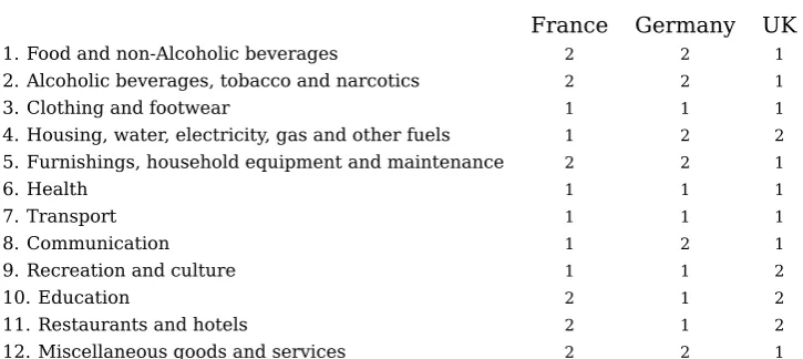
For the exercise we use the CPI data for France, Germany and the United Kingdom disaggregated to twelve components. The data is quarterly and seasonally adjusted, spanning from 1991 to 2015 and available from the OECD statistics database.15

[image:16.595.86.516.397.479.2]

The breakdown of the aggregate is the following:

Table 1: Components Breakdown

1. Food and non-Alcoholic beverages 7. Transport 2. Alcoholic beverages, tobacco and narcotics 8. Communication 3. Clothing and footwear 9. Recreation and culture 4. Housing, water, electricity, gas and other fuels 10. Education

5. Furnishings, household equipment and maintenance 11. Restaurants and hotels

6. Health 12. Miscellaneous goods and services

3.2

Forecasting models

Autoregressive model of order one (AR1)

Many of the aggregate-disaggregate forecasting competitions mentioned in the literat-ure review use univariate autoregressive methods and therefore we do so too. Regard-less of the numerous developments in econometric modelling, they continue to perform well (Marcellino, 2008). In particular, we use an autoregressive model of order one,

14

That is, we compare the improvement of the grouping against the corresponding direct and bottom-up approach as opposed to finding the best aggregation from the pool of alternatives for both AR(1)’s and BVAR’s.

x

i,t

=

a

i

+

ρ

i

x

i,t−1

+

ǫ

i,t, for the variables made stationary through differentiation

accord-ing to unit root tests.16 The forecasts are then produced using:

ˆ

x

_i,t+1|t

= ˆ

a

i

+ ˆ

ρ

i

x

i,t

Bayesian VAR (BVAR)

We do acknowledge, however, that interdependencies among components could play an important role, so we also use Bayesian Vector Autoregressive models (BVARs) follow-ing the implementation in Banbura et al. (2010). In practice, we forecast the whole multivariate process using five lags and the choice of overall tightness, as in Banbura et al. (2010), that produces the same in-sample of that of the direct aggregate forecast.

The estimated model is

X

t

=

c

+

A

1

X

t−1

+

. . .

+

A

5

X

t−5

+

ǫ

t

and the forecasts are produced using

ˆ

X

t+1|t

=

ˆ

c

+ ˆ

A

1

X

t

+

. . .

+

A

ˆ

5

X

t−4

3.3

Forecasting Accuracy Comparison

3.3.1 Set-up of the Evaluation Exercise

The evaluation exercise is performed over the 2001-2015 period leaving the first ten years of data to estimate the models. It is set up in a quarterly rolling scheme using a ten year window where in each period the models are re-estimated and a one-step-ahead forecast is generated.

The forecasting accuracy is presented by means of the model’s mean square forecasting error (MSFE) relative to that of a benchmark model. That is, for variable

i

and using model

m, the relative MSFE is

RelMSFE

(i,m)

=

MSFE

(i,m)

T0,T1

MSFE

(_Ti,₀0)_,T1

with

MSFE

(_Ti,m_0,T)₁

=

1

T

1

−

T

0

+ 1

T1

X

t=T0

y

_i,t(m₊₁)

|

t

−

y

i,t+1

2

where

y

_i,t(m₊₁)

|

t

is the forecasted value for

t

+ 1

at time

t

and

T

0 is the last period of actual

data in the first sample used for the evaluation and

T

1is the last period of actual data in

the last sample. As usual a RelMSFE lower than one reflects an improvement over the benchmark model for which

m

= 0

. To evaluate the significance of these differences, we compare the forecasts using the modified Diebold-Mariano test for equality of prediction mean squared errors proposed by Harvey et al. (1997).17

Regarding measuring the overall forecasting accuracy of the components we do so by comparing the cumulative absolute errors in the contribution to the aggregate level. For this purpose we define the cumulative absolute root mean square forecasting error for an aggregate with

N

components

q

n and using model

m

as

CumRMSFE

(_Tm_0,T)₁

=

v

u

u

u

t

1

T

1

−

T

0

+ 1

T1

X

t=T0 N

X

n=1

w

n,t+1

·

abs

q

_n,t(m₊₁)

|

t

−

q

n,t+1

!

2

where

q

_n,t(m₊₁)

|

t

is the forecasted value for

t

+ 1

at time

t

and

T

0is the last period of actual

data in the first sample used for the evaluation and

T

1is the last period of actual data in

the last sample.

3.3.2 Benchmark forecasting approaches

The objective of the whole exercise is to evaluate if there are successions of intermedi-ate aggregations that can improve overall forecasting accuracy as opposed to restrict-ing oneself only to usrestrict-ing either the direct or the full bottom-up approach. These two approaches are, therefore, the obvious comparison points.

We also acknowledge that Bermingham and D’Agostino (2014) find that the performance from the bottom-up approach could improve if the common features among components are accounted for. To see how our application measures up to an alternative approach we also compare it to a factor augmented autoregressive model. Following their im-plementation, we extend each univariate autoregressive model from the bottom-up ap-proach to include one factor

x

i,t

=

a

i

+

ρ

i

x

i,t−1

+

γ

i

F

t−1

+

ǫ

i,t

The factor,

F

, is estimated with the first principal component following Stock and Wat-son (2002) and computed over all components. The corresponding forecast for each

17

Table 2: Benchmark Forecasting Performance

France Germany UK

Bottom-Up AR(1) 0.91 0.95 0.88

Bottom-Up BVAR 0.95 0.94 1.17

Factor augmented AR(1) 0.91 0.98 0.88

Note: Root mean squared forecasting error relative to the direct method. * and ** denote significance of the forecasting performance difference based on the modified Diebold-Mariano test at a 10 and 5% significance level. Calculated over 2001-2015.

component is generated using

ˆ

x

F AAR_i,t+1|t

= ˆ

a

i

+ ˆ

ρ

i

x

i,t

+ ˆ

γ

i

F

ˆ

t

3.4

Results

3.4.1 Forecasting Performance Comparison

A first step to look at the results of the grouping methods is to evaluate how the benchmark models perform. In particular, Table 2 shows what would be a traditional aggregate-disaggregate comparison for the three series by presenting the root mean squared forecasting error of the direct and bottom-up approaches. It also presents the results for the factor augmented AR models to have a notion of whether the suggestion by Bermingham and D’Agostino (2014) can improve the univariate bottom-up methods in these particular settings.

We see that in five out of six of the cases the respective bottom-up approach performs better than the direct approach. In particular, the univariate approach tends to do better than the BVARs with improvements going from 5 to 12%, while the BVAR’s improve for France and Germany, about 5%, but do quite a bit worse than the direct method for the UK. In regards to the factor augmented AR, it does not seem to give any advantage to the simple AR. Although some of the differences could seem quite large, it is worth noting that they are not statistically significant.

[image:20.595.82.517.290.543.2]

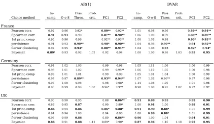
Table 3: Relative Forecasting Errors

AR(1) BVAR

In- Diss. Prob. In- Diss. Prob.

Choice method samp. O-o-S Thres. crit. FC1 FC2 samp. O-o-S Thres. crit. FC1 FC2

France

Pearson corr. 0.92 0.96 0.92* 0.89** 0.92** 1.01 0.98 0.96 0.89** 0.91**

Spearman corr. 0.91 0.91 0.98 0.87** 0.90** 1.06 1.09 0.99 0.88** 0.89**

1st princ.comp 0.96 0.96 0.99 0.92** 0.93** 1.00 1.03 0.98 0.93* 0.92**

persistence 0.91 0.93 0.90** 0.90* 0.90** 1.04 0.98 0.90** 0.94 0.92**

f-error clustering 0.92 0.95 0.94* 0.88** 0.91** 1.04 1.08 0.93 0.92* 0.94*

Bayesian 0.89* 0.93 0.92 1.02 0.92 0.94 1.00 1.00 0.98 1.03 0.95 0.95 Germany

Pearson corr. 0.98 1.02 1.00 0.99 0.98 1.05 1.11 1.06 1.00 0.99

Spearman corr. 0.98 1.01 1.02 0.99 0.98** 1.06 1.12 1.05 1.00 0.98

1st princ.comp 0.99 1.01 1.01 0.99 0.99 1.05 1.01 1.04 1.00 0.99

persistance 0.97 0.97 0.89** 0.93** 0.94** 1.07 1.02 0.96** 0.97 0.96

f-error clustering 0.97 1.00 0.98 0.98 0.98* 1.14 1.08 1.00 1.01 0.98

Bayesian 0.98 0.99 0.96 1.00 0.96* 0.97* 0.98 1.08 0.95 1.02 0.97 0.97

UK

Pearson corr. 0.90 0.90 0.95 0.88 0.86** 0.91 0.88 0.93 0.95 0.90

Spearman corr. 0.89 0.95 0.87 0.90 0.89* 1.00 0.91 1.00 0.98 0.91

1st princ.comp 0.86 0.94 0.86 0.86* 0.88* 0.91 0.90 0.88* 1.01 0.99

persistance 0.94 0.94 1.00 0.94 0.90 1.00 0.99 0.88* 1.01 0.99

f-error clustering 0.96 0.99 0.86 0.89 0.86** 0.96 1.00 1.04 0.94 0.91

Bayesian 0.86 0.91 0.88 1.11 0.89* 0.90* 0.87 0.94 1.16 1.18 0.95 0.95

the direct and full bottom-up approaches, but in some cases the performance is worse than that of either non-grouping methods.

If we go into the details, we find that for France the forecast combination choice meth-ods perform well overall. They provide improvements for most dissimilarity measure-ment choices and, although not necessarily large in magnitude, these improvemeasure-ments are statistically significant. In regards to the other choice methods, the coupling of the persistence dissimilarity measure and the dissimilarity threshold choice method per-forms well. All this is true for both the AR and BVARs. A difference, however, arises for the other choice methods between the forecasting models. For the AR all but the probabilistic choice improve on the direct method, while for the BVAR many methods do worse.

For Germany, the assessment is rather different. Few methods improve on the best non-grouping method and many are worse than either the direct or bottom-up approaches. However, even if the overall performance is poor, the forecast combination choice meth-ods still perform better than most of the alternative methmeth-ods that goes to show their robustness. The exception to this poor performance are the methods that use the per-sistence dissimilarity measure where some statistically significant improvements are obtained. Again, the dissimilarity threshold choice method performs well. Regarding differences between the forecasting models, for the BVARs most methods perform worse than the direct approach .

For the UK the outcome for the two forecasting models is quite different so it is worth looking at them separately. First, the results for the ARs look similar to the previous cases. The magnitudes of the gains in accuracy are relatively small, but again the fore-cast combination choice methods produce statistically significant improvements. How-ever, in this case the dissimilarity threshold choice method performs well with all dissim-ilarity measure choices except the one using persistence as the dissimdissim-ilarity measure. For the BVARs, on the other hand, there are many methods that show larger gains, around 10% over the direct method. The combination of the persistence dissimilarity measure and the dissimilarity threshold choice method again shows improvements that are statistically significant, but, in this case, many of the other dissimilarity measure choices also show relevant improvements for one or more choice methods.

Table 4: Relative Performance of Grouping Methods

Average Percentage Deviation Average Rank Difference

From Best Method With Best Method

In- Diss. Prob. In- Diss. Prob.

Choice method samp. O-o-S Thres. crit. FC1 FC2 samp. O-o-S Thres. crit. FC1 FC2

Pearson corr. 7.0 8.5 8.3 4.4 3.8 15.7 19.8 19.2 9.7 8.7

Spearman corr. 9.4 11.1 9.5 4.8 3.5 18.0 22.2 21.0 11.2 7.0

1st princ.comp 7.2 8.8 7.1 6.2 6.1 16.2 20.5 16.0 13.7 14.0

persistance 9.9 8.4 3.3 5.8 4.7 18.8 17.3 6.7 11.2 9.2

f-error clustering 11.0 12.7 6.8 4.7 4.1 20.7 26.0 13.7 9.8 9.0

Bayesian 4.1 8.5 8.6 17.0 5.2 5.8 7.3 20.2 12.0 25.8 11.3 13.3

Note: Relative performance of the grouping methods as measured by the average deviation of the respective root mean squared forecasting error (RMSFE) relative to that of the best performing grouping method by category and as the average difference in rank according to RMSFE over the six sets of forecasts. Grouping method dissimilarity measures: Pearson correlation, Spearman correlation, Variance explained by the first principal component, similarity in persist-ance measured as the difference of the estimated rho for an AR(1), forecasting error clustering for AR(1), Bayesian Hierarchical Clustering. Choice methods: In-sample criterion, Out-of-sample criterion, dissimilarity threshold, Probabilistic Criterion, Forecast Combination method 1 and Forecast Combination method 2. In bold the best performers in each category. Calculated over 2001-2015.

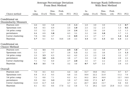
To evaluate these findings, Table 4 presents the relative performance of the 31 group-ing methods for the two forecastgroup-ing models and three countries.18 Two summarizing measures are presented. The first calculates the average over all six sets of forecasts of the deviation of the respective root mean squared forecasting error (RMSFE) from that of the best overall performing grouping method. The second, calculates the average difference in rank of the grouping methods, where the most accurate, in the RMSFE sense is ranked first and the least accurate is ranked last, 31st in this case. For both measures a smaller number means a more accurate model.

Both measures support the assessment made in the previous paragraphs. The method based on the persistence dissimilarity measure and the dissimilarity threshold choice criterion comes out best overall. Also, the forecast combination choice method per-formed better for all dissimilarity measure criteria, particularly the combination ap-proach that gives equal weight to each distinct forecast. Both measures, however, also point to the good performance of the combination of the Bayesian Hierarchical Cluster-ing and the in-sample choice criterion, somethCluster-ing that is not obvious at first sight from Table 3.

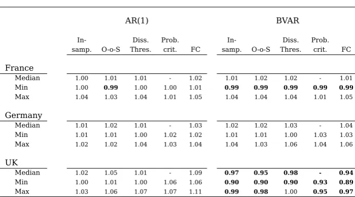
Regarding the accuracy of the components, Table 5 presents the median, minimum and maximum cumulative errors for each choice method relative to those of the bottom-up approach.19 _{For the first five sets of forecasts there is little difference between the}

cumulative forecasting errors of the grouping methods and the non-grouping methods and, in fact, some look marginally worse. On the contrary, for the case of the BVAR for the UK data, that happens to be the only case where the direct approach beats the bottom-up approach, the cumulative errors are reduced by as much as to 11% depending

18_{Results conditional on dissimilarity and choice methods are found in the Appendix in section B.2.} 19

[image:23.595.123.469.119.311.2]

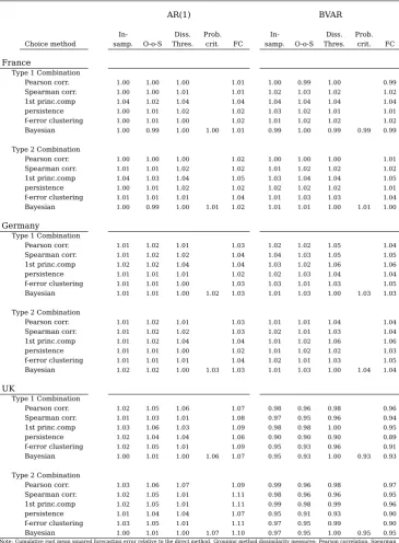
Table 5: Relative Cumulative Forecasting Errors

AR(1) BVAR

In- Diss. Prob. In- Diss. Prob. samp. O-o-S Thres. crit. FC samp. O-o-S Thres. crit. FC

France

Median 1.00 1.01 1.01 - 1.02 1.01 1.02 1.02 - 1.01

Min 1.00 0.99 1.00 1.00 1.01 0.99 0.99 0.99 0.99 0.99

Max 1.04 1.03 1.04 1.01 1.05 1.04 1.04 1.04 1.01 1.05

Germany

Median 1.01 1.02 1.01 - 1.03 1.02 1.02 1.03 - 1.04

Min 1.01 1.01 1.00 1.02 1.02 1.01 1.01 1.00 1.03 1.03

Max 1.02 1.02 1.04 1.03 1.04 1.04 1.03 1.06 1.04 1.06

UK

Median 1.02 1.05 1.01 - 1.09 0.97 0.95 0.98 - 0.94

Min 1.00 1.01 1.00 1.06 1.06 0.90 0.90 0.90 0.93 0.89

Max 1.03 1.06 1.07 1.07 1.11 0.99 0.98 1.00 0.95 0.97

Note: Cumulative root mean squared forecasting error relative to the direct method. Median, minimum and maximum values obtained from all grouping method dissimilarity measures and multilevel forecast combination methods. Choice methods: In-sample criterion, Out-of-sample criterion, dissimilarity threshold, Probabilistic Criterion. In bold CumRMSFE lower than that of the respective full Bottom-Up approach. Calculated over the 2001-2015.

on the grouping and choice method.

All this suggests that the grouping methods can improve overall accuracy. However, no dissimilarity measure for grouping nor aggregation level choice method by themselves clearly dominated the rest. From the individual and average results, however, in terms of disaggregation level selection, the dissimilarity threshold criterion used with either the first principal component, persistence or forecasting error clustering dissimilarity measures tended to outperform the others. For the forecast combination choice meth-ods, all dissimilarity measure choices performed relatively well.

As it is the case in most empirical applications, the impact of the grouping methods depends on the specific dataset. In particular, improvements in disaggregate accuracy were obtained only in the case where the direct approach was better than the bottom-up approach. It was also in this case that relatively more non-combination grobottom-uping methods improved aggregate accuracy. This could suggest that it is in settings like this, where the methods have a better chance of producing improvements. Such a result would not be entirely surprising, given the motivation for using dynamic grouping in the first place; that is to capture disaggregate dynamics in cases where full disaggregation could introduce to much noise.

in terms of disaggregate accuracy there were hardly any gains, in many cases the ac-curacy was similar to that of the best non-grouping method.

4

Conclusions

This paper presents a framework to forecast economic aggregates based on purpose built groupings of components. The idea underpinning this approach is that there are reasons that support both forecasting an aggregate directly and as the sum of its ponents. In particular, the literature emphasises the importance of accounting for com-monality among components, so we focus on this feature. To produce the groupings we follow a two-stage approach. First, we reduce the dimension of the problem by selecting a subset of possible groupings through the use of agglomerative hierarchical clustering. The second step involves producing the definitive forecast either by choosing the appro-priate grouping from the subset or combining them.

The results from the empirical application support that grouping methods can improve overall accuracy. On the one hand, some of the methods that selected a unique grouping performed better than the best performing non-grouping method. On the other hand, the forecast combination choice methods performed well overall. The exercise, however, contemplated only moderate disaggregation for the bottom-up approaches in which the biggest improvements were observed in the case where the bottom-up approach was less accurate than the direct approach. Espasa and Mayo-Burgos (2013) and Berming-ham and D’Agostino (2014) encourage using the maximum disaggregation possible in order to benefit from the disaggregate dynamics. All this suggests, that the method could perform well in a context of higher disaggregation.

Appendix

A

Empirical Framework

A.1

Multilevel combination where each unique forecast is given equal

weights

In this section we show how we implement the multilevel combination of the hierarchy, where each unique forecast is given equal weights. To do this we first show that, for the case of equal weights, combining the aggregate forecasts produced from different aggregation levels can be equivalent to deriving a set of component forecasts that are consistent with different aggregate forecasts combining them to produce a definitive bottom-up forecast. With this, each distinct combined component forecasts can be used to produce the combination where each unique forecast is given equal weights.

A.1.1 Joint combination using the lowest level of aggregation

Let there be a single aggregate forecast

y

and a single set of disaggregate forecasts

q

n

for

n

= 1

to

N

, the aggregate reliability weight

ϕ, the disaggregate reliability weights

φ

n and the aggregation weights

w

n. Cobb (2017) present a framework for multilevel

forecast combination, where the combined aggregate forecast is given by:

˜

y

=

Q

2

+

y

P

N n=1

ϕ φn

w

n

q

n

Q

+

P

N n=1

ϕ φn

w

n

q

n

(1)

where

Q

=

P

N

n=1

w

n

q

n.

They show that equation 1 is equal to the result of the equal-weight combination when all forecasts are assigned the same reliability. In this framework, the components are obtained from:

˜

q

n

=

1 +

ϕ

φ

n

y

−

Q

Q

+

P

N

n=1

ϕ φn

w

n

q

n

!

q

n (2)

be rewritten as follows:

˜

q

n

=

1 +

_φϕ

n

·

y−Q Q+PNn=1

ϕ φnwnqn

q

n

=

1 +

ϕ φn·(y−Q)

Q+PNn=1

ϕ φnwnqn

q

n

=

1 +

1

φn·(y−Q)

1

ϕQ+

PN

n=1_φn1 wnqn

q

n

Then, if we simply want to have a disaggregate scenario that is consistent with the original forecast

y, we take

q

n, for

n

= 1

to

N

, as the best guesses by setting the

aggregate reliability to infinity,

ϕ

→ ∞

. With this, we have:

ˆ

q

(ny)

=

1 +

y−Q

φn·PNn=1φn1 wnqn

q

n (3)

If we now combine the original forecast for the components with the consistent-with-y forecast for the component we get:

˜

q

alt

n

=

φnqn+ϕˆqn(y)

φn+ϕ

=

φnqn+ϕqn+ ϕ(y−Q) φn·PN_n=1

(

1

φnwnqn

)

·qn

φn+ϕ

=

1 +

_φϕ

n

·

y−Q

(φn+ϕ)PNn=1φn1 wnqn

q

n

that is slightly different from

q

˜

n. For equal weights among components, however, that

is

φ

n

=

φ:

˜

q

alt

n

=

1 +

ϕ_φ

·

y−Q

(φ+ϕ)1

φ

PN n=1wnqn

q

n

=

1 +

_φ+ϕ_ϕ

·

y−_QQ

q

n

=

Q(φ+ϕ_φ)+_+ϕϕ(y−Q)

qn

Q

=

φQ_φ++_ϕϕy

qn

Q

and by summing up the components we get that the aggregate is:

˜

y

=

φQ

+

ϕy

φ

+

ϕ

that is the same that you get from setting

φ

n

=

φ

for the standard result for the

aggreg-ate forecast.

This is a useful result for only one level of disaggregation, but the process is in fact extendible to unlimited exhaustive groupings of components.

guess of the decomposition of any sub-aggregation

y

s,k can be found using the equation

3. That is:

ˆ

q

(ys,k)

n

=

1 +

ys,k−Qs,k

φn·χs,k

q

n

with

χ

s,k

=

P

qn∈ys,k

1

φn

w

n

q

nand

Q

s,k

=

P

qn∈ys,k

w

n

q

n.

Then the definitive forecasts for the component is:

˜

q

n

=

φnqn+ S

P_ϕ

s,kqˆ

(_ys,k)

n

φn+ S

P

ϕs,k

=

"

1 +

1

φn+ S

P

ϕs,k

·

S

P

ϕs,k

φn

·

ys,k−Qs,k

χs,k

#

q

n

Then, for the case where all forecasts within the same grouping have the same reliabil-ity, we have that the aggregate is given by:

˜

y

=

N

X

n=1

w

n

"

1 +

1

φ+ S P_ϕ s

·

S

P

ϕ

s

·

ys,k−_QQs,k

s,k

#

q

n

=

Q

+

1

φ+PSϕs

·

S

P

ϕ

s

·

N

X

n=1

w

n

_y s,k

Qs,k

·

q

n

−

q

n

=

1 φ+ S P ϕs

·

"

Q

φ

+

S

P

ϕ

s

−

S

P

ϕ

s

Q

+

S

P

ϕ

s Ks

X

k=1 ys,k

Qs,k

·

P

qn∈Qs,k

w

n

q

n

!#

=

1 φ+ S P ϕs

·

"

φQ

+

P

S

ϕ

s Ks

X

k=1

y

s,k

#

By making

Y

s

=

Ks

X

k=1

y

s,k, it becomes clear that the definitive forecast is a weighted

aver-age of all the aggregate forecasts:

˜

y

=

φ

Q

+

S

P

ϕs

Y

s

φ+

S

P

ϕs

[image:28.595.197.396.118.288.2]

Figure 2: Aggregation levels on a dendrogram

A.1.2 Multilevel Combination counting each distinct forecast only once

The previous section shows the desired equivalence between taking the simple average of all the aggregate forecasts and the simple average for the components that have been reconciled with the original forecasts for the different levels of aggregation. This is useful because it permits building a best guess underlying scenario for the aggregate forecasts, but it implicitly gives higher reliability weights to components that are fused later in the algorithm if the component forecasts are generated independently. This can be visualized by looking at the dendrogram in Figure 2.

On this dendrogram we have drawn horizontal lines every time a fusion occurs to illus-trate the twelve options for groupings and the corresponding dissimilarity thresholds. At the very top we have the aggregate and at the very bottom all of the components in their own cluster. Let us denominate an aggregate forecast for a given grouping by the number of fusions that have occurred in that grouping. Using the nomenclature from the previous sections and assuming for simplicity that the aggregation weights,

w, are

all equal to one, the full bottom-up forecast is the sum of the forecasts of the individual components

q

nfor

n

= 1

to

N

. That is

Q

=

Q

(0)

=

P

N_n=1

q

n(0).

For all other aggregation levels, we can use the procedure described in A.1.1 to obtain forecasts of components that are consistent with the level of aggregation. For example, the forecast for the aggregation level that includes only the first fusion is produced from

Q

(1)

=

P

N

n6={2,5}

q

(1)

n

+

Q

{2,5}where

Q

{2,5}is the forecast of the sum of components 2 and

5 and

P

n6={2,5}

q

(1)

n is the sum of the forecasts of all the remaining components. In this

case we only reconcile the forecasts

q

(0)₂ and

q

₅(0)with

Q

_{2,5}obtaining

q

˜

(1)₂ and

q

˜

(1)₅ . With this

Q

(1)

=

P

N

n6={2,5}

q

(1)

n

+ ˜

q

(1)₂

+ ˜

q

₅(1). We can then proceed in this fashion for every level,

finishing with the direct aggregate forecast given by

y

=

Q

(11)

=

P

N n=1

q

˜

(11)

We can denote the whole set of forecasts as:

q

=





























q

₁(0)

q

(0)₂

q

(0)₃

q

₄(0)

q

₅(0)

q

₆(0)

· · ·

q

₁₂(0)

q

₁(1)

q

˜

(1)₂

q

(1)₃

q

₄(1)

q

˜

₅(1)

q

₆(1)

· · ·

q

₁₂(1)

q

₁(2)

q

˜

(2)₂

q

(2)₃

q

˜

(2)₄

q

˜

₅(2)

q

₆(2)

· · ·

q

₁₂(2)

.. .

˜

q

₁(11)

q

˜

₂(11)

q

˜

(11)₃

q

˜

₄(11)

q

˜

(11)₅

q

˜

₆(11)

· · ·

q

˜

(11)₁₂





























where

∼

denotes component forecasts that are the result of reconciling the individual forecasts,

q

(0)n , with a forecast for an intermediate aggregate.

The equal-weighted aggregate forecast combination can be written as:

Q

=

h

1

· · ·

1

i









Q

(0) .. .

Q

(11)









=

h

1

· · ·

1

i

q









1

.. .

1









=

h

q

¯

1

· · ·

q

¯

12

i









1

.. .

1









where

q

¯

ndenotes the equal-weighted forecast combination for component

n.

If the forecasts are produced using a univariate model, all those that do not involve conciliation will be the same unless the model is changed purposefully for each level of aggregation. The same is true of fusions that are not fused again with other clusters at that aggregation level. In this case the set of forecasts would show a particular pattern in that the forecasts are unaltered in the next aggregation level unless there is a fusion:

q

Indep.

=





























q

₁(0)

q

₂(0)

q

₃(0)

q

₄(0)

q

(0)₅

q

₆(0)

· · ·

q

(0)₁₂

q

₁(0)

q

˜

₂(1)

q

₃(0)

q

₄(0)

q

˜

(1)₅

q

₆(0)

· · ·

q

(0)₁₂

q

₁(0)

q

˜

₂(2)

q

₃(0)

q

˜

(2)₄

q

˜

(2)₅

q

₆(0)

· · ·

q

(0)₁₂

.. .

˜

q

₁(11)

q

˜

₂(11)

q

˜

₃(11)

q

˜

₄(11)

q

˜

(11)₅

q

˜

(11)₆

· · ·

q

˜

(11)₁₂





























In this context, it becomes clear that the simple average of all aggregate forecasts impli-citly gives higher reliability weights to components that are fused later in the process. If we look at component twelve, we have that

q

¯

12

= 10

q

(0)12

+ ˜

q

(10) 12

+ ˜

q

(11)

12 . A false sense of

certainty is given to the original forecast meaning that the aggregate equal-weight com-bination does not satisfy the condition of giving equal weights to the distinct forecasts.

the repeated forecasts from the component averages. This can be done based on the dendrogram. For component three, for example, the component forecast for the aggreg-ate combination would be given by

q

¯

3

= 3

q

(0)3

+ 2˜

q

(3) 3

+ ˜

q

(5) 3

+ 2˜

q

(6) 3

+ ˜

q

(8) 3

+ 2˜

q

(9) 3

+ ˜

q

(11) 3 and

B

Empirical Application

[image:31.595.117.480.204.366.2]

B.1

Data Transformation

Table 6: Differentiation for Empirical Application

France Germany UK

1. Food and non-Alcoholic beverages 2 2 1

2. Alcoholic beverages, tobacco and narcotics 2 2 1

3. Clothing and footwear 1 1 1

4. Housing, water, electricity, gas and other fuels 1 2 2

5. Furnishings, household equipment and maintenance 2 2 1

6. Health 1 1 1

7. Transport 1 1 1

8. Communication 1 2 1

9. Recreation and culture 1 1 2

10. Education 2 1 2

11. Restaurants and hotels 2 1 2

12. Miscellaneous goods and services 2 2 1

[image:32.595.82.516.164.454.2]

B.2

Relative Performance of Grouping Methods

Table 7: Relative Performance of Grouping Methods

Average Percentage Deviation Average Rank Difference From Best Method With Best Method

In- Diss. Prob. In- Diss. Prob.

Choice method samp. O-o-S Thres. crit. FC1 FC2 samp. O-o-S Thres. crit. FC1 FC2

Conditional on Dissimilarity Measure

Pearson corr. 4.6 6.0 5.8 1.9 1.3 2.0 3.0 3.0 1.3 0.7

Spearman corr. 6.8 8.5 6.9 2.3 1.0 2.5 3.2 2.5 1.3 0.5

1st princ.comp 3.5 5.2 3.5 2.6 2.4 2.2 3.0 2.0 1.5 1.3

persistance 8.4 6.9 1.8 4.3 3.2 3.2 3.0 1.0 1.7 1.2

f-error clustering 7.8 9.6 3.7 1.6 0.9 2.3 3.7 1.7 1.2 1.2

Bayesian 1.7 6.1 6.1 14.6 2.8 3.3 1.5 3.5 1.5 4.8 1.5 2.2

Conditional on Choice Method

Pearson corr. 3.2 3.1 7.5 2.4 1.8 2.2 2.2 3.0 1.7 2.2

Spearman corr. 5.5 5.7 8.7 2.8 1.5 3.2 3.3 3.8 2.5 1.3

1st princ.comp 3.3 3.5 6.3 4.3 4.0 2.5 2.3 2.8 3.2 3.7

persistance 6.0 3.0 2.5 3.8 2.7 3.0 1.8 1.0 2.8 2.2

f-error clustering 7.1 7.3 6.0 2.7 2.0 3.5 3.7 2.2 2.0 2.3

Bayesian 0.3 3.1 7.8 3.2 3.8 0.7 1.7 2.2 2.8 3.3

Overall

Pearson corr. 7.0 8.5 8.3 4.4 3.8 15.7 19.8 19.2 9.7 8.7

Spearman corr. 9.4 11.1 9.5 4.8 3.5 18.0 22.2 21.0 11.2 7.0

1st princ.comp 7.2 8.8 7.1 6.2 6.1 16.2 20.5 16.0 13.7 14.0

persistance 9.9 8.4 3.3 5.8 4.7 18.8 17.3 6.7 11.2 9.2

f-error clustering 11.0 12.7 6.8 4.7 4.1 20.7 26.0 13.7 9.8 9.0

Bayesian 4.1 8.5 8.6 17.0 5.2 5.8 7.3 20.2 12.0 25.8 11.3 13.3

[image:33.595.115.481.159.656.2]

B.3

Relative Cumulative Forecasting Errors

Table 8: Relative Cumulative Forecasting Errors

AR(1) BVAR

In- Diss. Prob. In- Diss. Prob. Choice method samp. O-o-S Thres. crit. FC samp. O-o-S Thres. crit. FC

France

Type 1 Combination

Pearson corr. 1.00 1.00 1.00 1.01 1.00 0.99 1.00 0.99

Spearman corr. 1.00 1.00 1.01 1.01 1.02 1.03 1.02 1.02

1st princ.comp 1.04 1.02 1.04 1.04 1.04 1.04 1.04 1.04

persistence 1.00 1.01 1.02 1.02 1.03 1.02 1.01 1.01

f-error clustering 1.00 1.01 1.00 1.02 1.01 1.02 1.02 1.02

Bayesian 1.00 0.99 1.00 1.00 1.01 0.99 1.00 0.99 0.99 0.99

Type 2 Combination

Pearson corr. 1.00 1.00 1.00 1.02 1.00 1.00 1.00 1.01

Spearman corr. 1.01 1.01 1.02 1.02 1.01 1.02 1.02 1.02

1st princ.comp 1.04 1.03 1.04 1.05 1.03 1.04 1.04 1.05

persistence 1.00 1.01 1.02 1.02 1.02 1.02 1.02 1.01

f-error clustering 1.01 1.01 1.01 1.04 1.01 1.03 1.03 1.04

Bayesian 1.00 0.99 1.00 1.01 1.02 1.01 1.01 1.00 1.01 1.00

Germany

Type 1 Combination

Pearson corr. 1.01 1.02 1.01 1.03 1.02 1.02 1.05 1.04

Spearman corr. 1.01 1.02 1.02 1.04 1.04 1.03 1.05 1.05

1st princ.comp 1.02 1.02 1.04 1.04 1.03 1.02 1.06 1.06

persistence 1.01 1.01 1.01 1.02 1.02 1.03 1.04 1.04

f-error clustering 1.01 1.01 1.00 1.03 1.03 1.01 1.03 1.05

Bayesian 1.01 1.01 1.00 1.02 1.03 1.01 1.03 1.00 1.03 1.03

Type 2 Combination

Pearson corr. 1.01 1.02 1.01 1.03 1.01 1.01 1.04 1.04

Spearman corr. 1.01 1.02 1.02 1.03 1.02 1.01 1.03 1.04

1st princ.comp 1.01 1.02 1.04 1.04 1.01 1.02 1.06 1.06

persistence 1.01 1.01 1.00 1.02 1.01 1.02 1.02 1.03

f-error clustering 1.01 1.01 1.01 1.04 1.02 1.01 1.03 1.05

Bayesian 1.02 1.02 1.00 1.03 1.03 1.01 1.03 1.00 1.04 1.04

UK

Type 1 Combination

Pearson corr. 1.02 1.05 1.06 1.07 0.98 0.96 0.98 0.96

Spearman corr. 1.01 1.03 1.01 1.08 0.97 0.95 0.96 0.94

1st princ.comp 1.03 1.06 1.03 1.09 0.98 0.98 1.00 0.95

persistence 1.02 1.04 1.04 1.06 0.90 0.90 0.90 0.89

f-error clustering 1.02 1.05 1.01 1.09 0.95 0.93 0.96 0.91

Bayesian 1.00 1.01 1.00 1.06 1.07 0.95 0.93 1.00 0.93 0.93

Type 2 Combination

Pearson corr. 1.03 1.06 1.07 1.09 0.99 0.96 0.98 0.97

Spearman corr. 1.02 1.05 1.01 1.11 0.98 0.96 0.96 0.95

1st princ.comp 1.02 1.05 1.01 1.11 0.99 0.98 0.99 0.96

persistence 1.01 1.04 1.04 1.07 0.95 0.91 0.93 0.90

f-error clustering 1.03 1.05 1.01 1.11 0.97 0.95 0.99 0.90

[image:34.595.166.428.165.222.2]

B.4

Forecasting Accuracy Excluding Financial Crisis

Table 9: Benchmark Forecasting Performance Excluding Crisis

France Germany UK

Bottom-Up AR(1) 0.95 0.90 0.90

Bottom-Up BVAR 0.97 0.98 1.25

Factor augmented AR(1) 0.96 0.88* 0.90

Note: Root mean squared forecasting error relative to the direct method. * and ** denote significance of the forecasting performance difference based on the modified Diebold-Mariano test at a 10 and 5% significance level. Calculated over 2001-2015 excluding from 2008.III to 2009.II.

Table 10: Relative Forecasting Errors Excluding Crisis

AR(1) BVAR

In- Diss. Prob. In- Diss. Prob.

Choice method samp. O-o-S Thres. crit. FC1 FC2 samp. O-o-S Thres. crit. FC1 FC2

France

Pearson corr. 0.92 0.97 0.94 0.88** 0.90** 1.03 0.97 1.00 0.91* 0.93*

Spearman corr. 0.89* 0.90** 0.98 0.87** 0.89** 1.09 1.11 1.01 0.89** 0.91**

1st princ.comp 0.94 0.95 0.98 0.90** 0.92*