Munich Personal RePEc Archive
Crime, Transition, and Growth
Djumashev, Ratbek and Abdullaev, Bekzod
Monash University, RMIT University
17 August 2017
Online at
https://mpra.ub.uni-muenchen.de/80842/
Crime, Transition, and Growth
Ratbek Dzhumashev
∗and Bekzod Abdullaev
†Abstract
This paper analyses whether the effect of crime on growth depends on the structural changes caused by transition. The result of the simple model suggests that when the structure of economy changes, the cost of economically motivated crime will also change; thus, affecting the impact of crime on economic perfor-mance. Using data for some of the republics of the former Soviet Union, we find support for this conjecture.
Key words: growth, crime, transition economies
JEL Code:P26, P52, O57, O17
1
Introduction
Crime imposes significant costs on the society due to the consumption of illegal
products and/or the negative externality associated with illegal activities
(Czaban-ski, 2008). As a result of the significance of the economic costs of crime, over the last
three decades an increasing number of studies have focused on this topic. However,
despite the growing research in this field, so far no empirical study on the impact
of crime examines how the transition from a command economy to a market based
economy influences the effects of crime on growth.
In order to address the aforementioned gap in the existing literature, we analyse
how the structural changes occurred during transition influence the impact of crime
on growth. To guide our empirical analysis, we develop a simple growth model
where the criminal activities affect economic outcomes, given the costs associated
with the criminal activities. Namely, in the model, we link both the cost of criminal
∗
Department of Economics, Monash University, 100 Clyde Road, Berwick, Victoria 3806,
Aus-tralia,[email protected]
activity and the gains from it to the structure of the economy. Based on the analysis
of the model, we obtain some insights into how the effect of crime on the economy
may change as the structure of the economy changes. We then provide empirical
evidence on how the effect of crime on economic growth has changed in some of the
former USSR economies during the 1985-2010 transition that had led to a change in
the structure of the economy in those countries.
In building our model we employ the reasoning proposed in the extant literature.
Specifically, in his influential paper, Becker(1968) provides an economic rationale to
criminal activities as well as optimal policies to combat illegal behaviour; that is, the
criminals respond to economic incentives in the same way as the law-abiding
cit-izens. The results of the model predict that the law enforcement depends on the
probability of detection of a crime and the severity of the punishment. Ehrlich
(1973) theoretically models the participation of individuals in illegitimate
activi-ties, and tests his model using US state data. He finds that inequalities increase
the level of crime, especially crime against property; while, the probability of being
caught discourages the crime. We follow Becker (1968) and Ehrlich (1973) in terms
of determining the incidence of crime, but also extend their approach by assuming
that parameters such as the probability of detection or the cost of criminal activity
also depend on the institutional aspects of the economy. In addition, the structural
changes in the economy influence criminal activities by altering both the marginal
productivity of criminal effort and the costs associated with crime.
In existing empirical studies, the effect of crime on growth has not been found
to be unambiguously negative. For example, the World Bank study (2006), based
on data from 43 countries for 1975-2000, reports results suggesting a strong
nega-tive effect of crime on growth. Càrdenas (2007) also finds a significantly neganega-tive
association between crime and per-capita output growth in a panel of 65 countries
using homicide data for 1971-1999. On the other hand, Mauro and Carmeci (2007)
find that crime has a negative impact on income levels but exerts no significant
long-run adverse effect on growth rates. Moreover, most of the published literature
of crime; however, crime, as one of the determinants of economic growth, largely
remains neglected in the macroeconomic framework (Detotto and Otranto, 2010).
Olavarria-Gambi (2007) estimates an aggregate burden of crime for Chile in 2002 at
2.06 percent of the GDP.
As aforementioned, the relationship between crime and certain economic
indi-cators has been under some empirical scrutiny. One strand of the empirical studies
on the effect of crime attempted to explain the difference in economic performance
across countries due to the difference in the incidence of crime along with other
variables (Sandler and Enders, 2008; Barro, 1996; Gardenas, 2007; Gaibulloev and
Sandler, 2008). The other strand of the relevant empirical studies employ time series
estimation methods and examines whether there is a causal relationship between
crime and certain economic variables (Neanidis and Papadopoulou, 2013; Mauro
and Garmeci, 2007; Gardenas, 2007; Habibullah and Baharom, 2009; Detotto and
Pulin, 2009; Chen, 2009; Narayan and Smyth , 2004). Along the lines of the latter
literature, Detotto and Otranto (2010) address two questions: first, whether the
eco-nomic effect of crime depends on the level of the crime rate, and second, whether
crime affects the economy differently depending on the business cycle. However,
as there were no institutional changes in the subject country (Italy) during the
ex-amination period, Detotto and Otranto (2010) could not test the effect crime had on
growth as a result of changes in the structure of the economy. Given this gap in
the existing literature, this paper contributes by analysing and thus providing new
insights on the effect of crime on economic growth as a result of structural changes
in the economy.
Additionally, there are some shortcomings in the empirical literature stemming
from the use of proxies when it comes to crime rather than actual measures of
the degree of crime. Some studies (for example, Powell et al., 2010) using
cross-country data do not explicitly control for crime but instead use proxy variables such
as the "rule of law", "political stability", "civil liberties", "corruption rate",
"govern-ment leadership", "inequality" amongst other variables. We attempt to address this
number of crimes committed in country at a given period of time.
In terms of the broader framework pertaining to the analysis of economic growth,
our study is in line with the existing literature. In particular, Barro (1991) considers
various determinants of growth and finds that political instability negatively
influ-ences economic growth. In his study he uses two variables as measures of political
instability, the number of revolutions and coups per year and the number of political
assassinations per million of the population per year. He finds that across countries
both variables are statistically significant and negatively correlated with growth. In
another cross-country analysis of growth, Barro and Sala-i-Martin (1995) find that
political instability has a detrimental impact on growth, whereas a stronger rule of
law has a positive and significant effect on growth. Additionally, using a sample of
53 developing countries from 1984 to 1995, Poirson (1998) finds that stronger
eco-nomic security contributed significantly to private investment and growth.
Specif-ically, he finds that in the short run, reductions in expropriation risk and terrorism
influence growth positively, while in the long-run, corruption and contract
repudia-tion affect growth negatively in the long run. In view of the aforemenrepudia-tioned works,
the framework we employ in this study assumes that the general institutional
struc-ture significantly influence the effect of crime on economic growth.
While there are number of studies examining the effect of crime on growth in
developing economies, no study to date examines the effect of crime on growth in
a transitioning economy. It is well-known that in the former Soviet Union
coun-tries, there was an expansion of illegal activities during the early years of transition.
Shelly (1995) attributes this phenomenon to the insecurity of capital, money
laun-dering, the growth of organised crime and the ineffective policies that were in place
to fight crime in Russia and the Commonwealth of Independent States (CIS)
coun-tries. The transition caused deep structural changes that might have also affected
how the criminal operate in the former USSR countries. For example, the transition
affected the structure of property rights significantly due to the large scale of
pri-vatisation programs implemented in al of the former USSR countries. In fact, it has
were quite weak in most of the former Soviet economies (Sonin, 2003; Braguinsky
and Myerson, 2007a, 2007b). Although it has been highlighted that such economies
develop either a system with weak property rights and rent-seeking or with strong
property rights imposed by a dictator (see e.g. Hafer, 2006; Guriev and Sonin, 2009).
In light of this, our study attempts to gain new insights into the relationship between
crime and growth.
Our analysis yields the following results. The main result is that the private
property rights and other structural changes that emerged after the collapse of the
command economy played a positive role in decreasing the negative effect of crime
on economic growth. Specifically, we find that during the transition, decline in the
negative effect of crime can be attributed to the structural changes. This result is
indirectly supported by the finding of Detotto and Otranto (2010), who find
dur-ing recessions there in an increase in the negative effect of crime. Namely, given
that during the transition all the former USSR economies experienced an economic
recession, the expected increase in the negative effect of crime on growth was
less-ened by the structural changes in the economy. The main structural changes appear
to come in the form of increased productivity of crime (due to stronger
organisa-tion of crime) and reduced pool of felonious agents (most likely implemented by a
dictatorship-type governance). In addition, unlike Detotto and Otranto (2010), we
find that the marginal effect of crime depends on the level of crime. We explain this
difference as a result of the structural changes that had occurred during the
transi-tion of the economies of the former USSR that we consider in our empirical analysis.
2
Model
There are two types of agents: law-abiding and felonious. Assume that there is a
fixed measure of mass of citizens, λ, are potential criminals, while 1−λ are the
Criminal agent
A fraction ε ∈ (0, 1) of felonious agents choose to be criminal. Those who are a
criminal-type choose the level of their effort, φt ∈ (0, 1), in criminal activities. This
implies that the intensity of crime is determined byφtε. The criminals receive illegal
income from each victim, given asτt =θφt, where θ is the productivity of criminal
activities. One way to model this the productivity of criminals is to state it as a
function that depends on the wage rate in the economy, as with higher income of
the citizens, crime allows to capture more income for any given effort. We assume
thatθ =θ0wζt, where θ0and ζ <1 are parameters. There are n= 1−λ
ελ victims per a
given felonious agent.
The criminals can be detected with probability, p, for their crimes, and incur
costs, xt. The magnitude of this cost depends positively on the extent of the crime
and this cost is increasing with the income generated in criminal activities; that is,
the worse the crime the higher the cost. For tractibility sake, we assume that this
cost can be captured by a quadratic function of the income from criminal activities.
In addition, there is externality from the overall criminal rate in the economy. The
more agents choose to be criminal the less becomes the cost of criminal activity.
Therefore, the cost faced by a felonious agent is given by:
x=η(1−ε)τt2, (1)
whereηis an exogenous cost parameter. The probability of detection, p, along with
the parameters that drive the costs associated with crime depend on the economy’s
institutional setting.
We link the cost of crime to the structural changes that take place when an
econ-omy transitions from a command driven to a market driven econecon-omy. These
result-ing structural changes give rise to private property rights and protection, alterresult-ing
the cost of running criminal activities, and hence, the effect of crime on economic
growth. This conjecture is based on the following analytical findings.
command versus market-based, we use the rationale given in Besley and Ghatak
(2010). They argue that in an environment where public ownership of capital is
combined with a socialist regime, the wage rate would be set below the
incentive-compatible level. In our context, this can be expressed as the optimal wage rate with
some level of tax,π. In general, this formulation implies that the tax rate under the
command economy regime is higher than under the market economy regime. That
is, the effective wage rate for the agent is given as(1−π)wt, where wt is the gross
wage rate. However, this does not imply that the effective wage rate is lower
un-der command economy by definition, as the effective wage rate also depends on
the gross wage rate,wt. Therefore, even ifπ is higher in the command economy, if
the gross wage rate, wt, is high enough, then it is possible that the effective wage,
(1−π)wt, is higher than in a market economy with lower taxes and gross wage rate.
If an agent is engaged in criminal activities, then he or she can work in the official
sector. This does not look far fetched. However, given that part of their time is
dedicated to criminal activities, the time spent working in the legal sector should
decrease. In light of this discussion, the income of the felonious-type agent is given
by
(1−π)wt+rtk1t with prob.(1−ε)
(1−φ)(1−π)wt+rtk1t +φ[nτt−pxt] with prob. ε
wherert is the rate of return to capital andkt is the stock of capital per worker.
Given this, the felonious-type agent solves the following problem:
max
c,φ,ε U=
∞
Z
0
ln(c1t)e−ρt
dt, (2)
s.t.
˙
k1t= (1−π)wt(1−εφt) +rtk1t+φ(nτt−pxt), (3)
τt=θφt, (4)
To solve this problem, we construct a present-value Hamiltonian:
H=ln(c1t)e−ρt
+v1[(1−π)wt(1−φtε) +rtk1t+ε(nτt−pxt)]. (6)
The first-order conditions with regard to choice and state variables yield the
follow-ing:
∂H
∂c1t =
e−ρt
c1t
−v1=0. (7)
∂H
∂φ =v1
h
−(1−π)wtε+ε
nθ−2pη(1−ε)θ2φt
i
=0. (8)
∂H
∂ε =v1
h
−(1−π)wtφ+ε
pη(θφt)2
i
=0. (9)
−v˙1= ∂H
∂k1t
⇒v˙1=−v1rt. (10)
From (8) we obtain the equilibrium share of criminal agents:
−(1−π)w+ (nθ−2pη(1−ε)θφ) =0.
Solving this forε,
ε∗
t =1−
(1−π)wt−ηθ
2pηφθ . (11)
Solving (9), we write:
ε∗
=(1−π)w
pηφθ2 (12)
Equalising (11) and (12) we write:
1−(1
−π)wt−ηθ
2pηφθ =
(1−π)w
pηφθ2 . (13)
Solving (13) forφwe obtain:
φ∗= (1−π)w(2+θ) +nθ
2
2pηθ2 . (14)
By analysing (14) and accounting forθ=θ0wζt, we can state the following.
de-creases if otherwise. An increase in the cost of criminal activities or the probability of
detec-tion, reduces criminal effort.
By substituting forφin (12) we obtain:
ε∗
= 2(1−π)w
(1−π)w(2+θ) +nθ2. (15)
Now, using (15), we state the following.
Lemma 2.2 The incidence of crime,ε, decreases together with the wage rate. An increase in
the spread of crime (lower n), increases the incidence of crime.
Accounting for θ =θ0wζt and using (14) and (15), we write that the optimal
in-tensity of crime,φ∗
ε∗
, as follows:
φ∗
ε∗
= (1−π)w1
−2ζ
pηθ20 (16)
Analysing the equilibrium value of the criminal intensity given above, we can
state the following:
Proposition 2.3 The criminal intensity decreases with the productivity of crime stemming
from institutional setting,(θ0), tax burden , (π), the probability of detection (p), and the cost
associated with the crime (η). On the other hand, the criminal intensity increases with the
wage rate, w, ifζ<1/2, and decreases ifζ>1/2.
Proof The result is straightforward by considering the comparative statics of (16).
The above result indicates that a transition to a market economy as a result of an
increase in the effective wage rate raises both the opportunity cost of crime and
its productivity. However, which effect dominates is determined on whether the
marginal elasticity of productivity of crime is higher than a certain threshold or not;
that is, if ζ >1/2 holds or not. Apparently, the productivity of crime depends on
the institutional environment. Thus, if the institutional setting is not facilitating for
criminal activities then rising wage rates result in falling criminal intensity. In
associated with the criminal activities may rise due to a increase the value of
param-eter θ0. The value ofθ0 may increase by weakened property rights and growth of
organised crime (Shelly, 1995; Sonin, 2003; Braguinsky and Myerson, 2007a, 2007b),
or it may decrease if the form of governance turns into a dictatorship type (Guriev
and Sonin, 2009). Whether these effects of structural changes actually take place is,
of course, an empirical question, which we will deal with in section 3.
Law-abiding agent
The law-abiding agent works full time at the firm and rents out all his capital to the
firm. If this agent falls victim to a criminal act with the probability of q, the agent
will incur a loss of his or her income, given by τ. The agent solves the following
problem:
max
c U1=
∞
Z
0
ln(c2t)e−ρtdt, (17)
s.t.
˙
k2t = (1−π)wt +rtk2t−qτ, (18)
q= ε(1−λ)
λ . (19)
It can be verified that the optimisation problem faced by this type of agent leads to
a similar consumption growth rate as that of the felonious agent. That is,
˙ c2t
c2t =r−ρ. (20)
The firm
Due to constant returns to scale we can assume that there is only one firm in the
economy, which operates based on the following technology:
Yt=AKtα(Lt(1−φε))1
−α
whereAis the productivity coefficient,Ktis the aggregate stock of capital,Ltis total
labour, 0<α<1 is the output elasticity of capital . In per capita terms, we can write
yt =Akα(1−φε)1
−α
. (22)
We assume that the productivity coefficientA=A(φε)is such thatA′
φε<0,A′′φε<
0. The firm maximises its profits according to the following:
max
k
Π=Akαt(1−φε)1−α−(1−π)wt(1−φελ)−rkt. (23)
The solution to this problem is given as:
∂Π
∂k =0⇒rt =Aαk
α−1
t (1−φε)1
−α
. (24)
The growth rate
Let us consider the effect of crime on the growth rate defined by equation (20). This
analysis leads to the following proposition.
Proposition 2.4 If the intensity of crime is falling in the wage rate (ζ>1/2), the negative
effect of crime on economy’s growth is declining with further growth. However, this also
implies that if the intensity of crime is rising in the wage rate (ζ <1/2), then the negative
feedback from crime to economic growth can limit growth rates and create a trap.
Proof Combining (17) and (24) we can write the growth rate of the economy as:
g= c˙t
ct =Aαk
α−1
t (1−φε)
1−α
−ρ.
It can be verified that ∂(∂φεg) <0. Therefore, if economic growth that leads to higher
effective wage rates,(1−π)w, also reduces the intensity of crime (i.e. ∂(φε)
∂w <0), then
both crime levels and its effect on economic growth decline. On the other hand, if
economic growth leads to a higher intensity of crime due to the condition ∂(∂φεw) >0
holding, then this negative feedback would limit the rate of economic growth due
3
The Empirical Framework
We derive the empirical model from the above theoretical findings using the
method-ology employed by Mankiw et al (1992), MRW hereafter. Let us denote
ˆ
kt = Kt
ALt, (25)
ˆ
yt = Yt
ALt
=kˆα(1−φε)1−α. (26)
The capital accumulation equation can be written as,
˙ˆ
kt =ityˆt−(n+δ)kˆt, (27)
whereit is the share of investment in total output,nis the rate of population growth,
δ is the depreciation rate of capital. Following MRW, we consider the steady-state
growth rate, where ˙ˆkt = 0. Then from (27) we find the capital stock per unit of
effective worker
¯ˆ
kt =
it
n+δ
1−1α
(1−φtε). (28)
By inserting the above expression for the steady state value of capital back into (26)
and taking logs, the steady state value of income per capita is derived as:
log ˆy∗
t =
α
1−αlogit − α
1−αlog(n+δ) +log(1
−φtε). (29)
This is the well-known empirical growth equation used by Mankiw et al. (1992).
This approach has been extended by Islam (1995) who demonstrates that the model
can be adjusted for panel data by approximating the pace of convergence around
the state level of output,y∗
. This gives us a dynamic model where the adjustment
process towards the state is given by:
lnyˆt = (1−e
−π
where π= (n+δ)(1−α). After rearranging and substituting fory∗ from (29), we
arrive at:
lnyˆt−lnyˆt−1= 1−e −π
α
1−αlni − α
1−αln(n+δ) +log(1
−φtε)−lnyˆt−1
(30)
By noting that lnyˆt =lnyt −lnA, where yt =Yt/Lt, (30) is transformed into the
following form:
lnyt = 1−e−π
α
1−αlni − α
1−αln(n+δ) +log(1
−φtε)
−e−π(lnyt−1+lnA).
(31)
The panel-data empirical model based on the above equation can be expressed in a
conventional form as follows:
yjt=γyj,t−1+
3
∑
m=1
βjXmjt +µj+νjt, (32)
where yjt =lnyt, yj,t−1 =lnyj,t−1, γ =−e −π
, β1 = (1−e−π) α
1−α
, β2 = −(1−
e−π
) 1−αα
, β3=1−e−π, x1jt =lnijt, x2jt=ln(njt+δ), x3jt=ln(1−φjtεj), and µj=
−e−πlnA. The stochastic disturbance terms are assumed to satisfy the following:
E[µj] =E[νjt] =E[µjνjt] =0.
Since, the intensity of crime, φε is not directly observed, we use the crime rate
as a proxy. Hence, instead of ln(1−φε), we use ln(Crime). To determine the
condi-tions under which crime affects growth, we modify the basic empirical model (32)
by taking into account that the TFP, A, is a function of the crime rate. Specifically,
we postulate that the dependence between productivity and crime may change as a
result of the structural changes in the economy. In the empirical model, we
imple-ment this rationale by adding an interaction term between a dummy variable (equal
to 1 for post-Soviet period) and the crime rate. This dummy variable captures the
structural changes that take place during the transition period. The robustness of
the results is verified using the property rights indicator defined as the share of the
4
Data and Estimation
Several sources of data have been utilized in this study. The annual GDP series and
Population figures are collected from the Maddison dataset (Bolt & van Zanden,
2013). Net capital formation (investment) series are from the Official Statistics of the
Countries of the Commonwealth of Independent States (CISStat, 2013).1 As
afore-mentioned, the crime rate is used as a proxy for criminal intensity and is obtained
from CISstat for the entire period. The crime rate is calculated per 100,000
popu-lation (that is, Total number of Crimes/Popupopu-lation x 100,000) and includes crimes
such as first degree/premeditated murder (including attempted), grave bodily
in-juries, thefts, robbery, bribery and crimes associated with narcotics. Crimes related
to hooliganism and rape have been excluded as these crimes are not necessarily
driven by economic incentives.
Using a total number of criminal acts as a measure of crime might be questioned
on the grounds that the different types of crime can have different prevalence and
economic consequences. However, when one is focused only on the incidence of
crime but not its nature (as soon as it has some economic consequence), using the
total numbers of criminal acts should be fine. As for the structural changes in
crimi-nal activity, we intend to gauge that through estimating its impact on overall income
measured by GDP. For estimation purposes, all series are transformed into
logarith-mic form. Following other studies in this area (see, for example, Schündeln, 2013)
the depreciation rate is set at a constant rate of 10 per cent for all countries. As a
re-sult of the scarcity of data for some countries, the sample contains the following 10
countries: Armenia, Azerbaijan, Belarus, Kazakhstan, Kyrgyzstan, Moldova,
Rus-sia, Tajikistan, Ukraine and Uzbekistan. The dataset contains 260 observations and
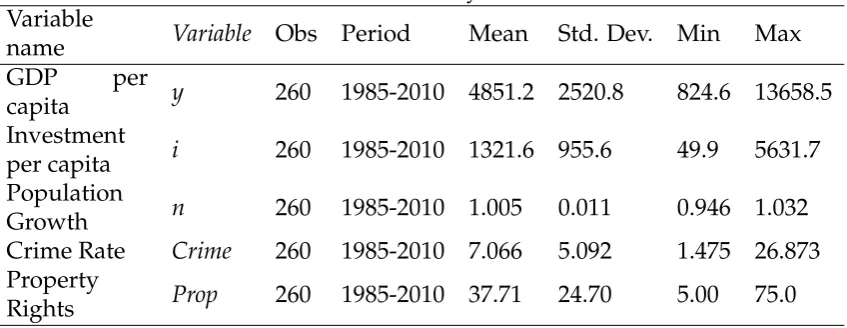
covers the following time period, 1985-2010. Table 1 presents the summary statistics
of all the model variables.
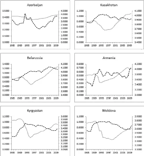
Figure 1 exhibits the pattern of the crime rate and GDP per capita for the
coun-tries in the sample from 1985 to 2010. It is interesting to note that the crime rate
1The official statistics for net capital formation divided into two periods: pre- and post USSR
Table 1: Summary Statistics Variable
name Variable Obs Period Mean Std. Dev. Min Max
GDP per
capita y 260 1985-2010 4851.2 2520.8 824.6 13658.5 Investment
per capita i 260 1985-2010 1321.6 955.6 49.9 5631.7 Population
Growth n 260 1985-2010 1.005 0.011 0.946 1.032 Crime Rate Crime 260 1985-2010 7.066 5.092 1.475 26.873 Property
Rights Prop 260 1985-2010 37.71 24.70 5.00 75.0
(dashed line) has been increasing in all of the CIS countries prior to the collapse of
the USSR. After the USSR collapse, a sharp decline can only be observed in
Azer-baijan (1993-2000), in Tajikistan (1993-2008) and in Uzbekistan (1993-1995). It is also
evident that in all countries, with the exception of Tajikistan and Uzbekistan, the
post USSR crime rate on average is higher than the crime rate that prevailed during
the USSR.
In terms of economic growth, almost all countries experienced a decline during
the first few years of the transition. Some of the countries recovered from the
prob-lems of high inflation, low manufacturing, chaotic budget structures and declining
trade, by the mid 1990s; whereas sin countries such as Russia, Moldova and the
Ukraine, stagnation was observed up until 1998. Following the recovery from the
Russian financial crisis of 1998, robust economic growth was observed in all of the
CIS countries. The average growth rate between 2000 and 2008 was over 6 per cent.
This was a result of macroeconomic stability, high foreign investment, a decline in
government expenditures, fiscal discipline and tax reforms, rising energy exports,
structural reforms in manufacturing, agricultural and service sectors, as well as the
liberalization of trade in the major the CIS countries. The effects of the Global
Finan-cial Crisis on the CIS countries were minimal as the finanFinan-cial institutions were not
exposed directly to US credit markets. The CIS countries have been mostly affected
by the falling commodity prices, as a result of the global slow down in demand for
exports from these economies.
the conventional OLS estimates. In the case of the OLS estimates, we estimate Eq.
(27) using the fixed (FE) and the random effects (RE) estimator without the USSR
dummy, column 1 and 2, respectively; and, with the post-USSR dummy (1 for years
after 1991, and 0 otherwise), column 3 and 4, respectively. In order to address the
problem associated with country specific effects and the regressors, as highlighted
by Baltagi (1995) and Roodman (2009), we conduct a Hausman test. The result of
the Hausman test (Davidson and MacKinnon, 1982, 1993) shows that the
country-specific effects are correlated with the regressors in our model at least at the 5 per
cent significance level. Thus, the RE estimator is rejected in favour of the FE
es-timator. However, due to the presence of the lagged growth variable, the FE is
inconsistent (Baltagi, 1995).
Given the inconsistency of the FE estimator, in the presence of a lagged
endoge-nous variable, the potential endogeneity of other regressors and the number of
in-struments, we employ the system Generalized Method of Moments (GMM)
esti-mator for dynamic panel data.2 We use the GMM estimator, following Arellano
and Bover (1995) and Blundell and Bond (1998), as it allows us to obtain
consis-tent and efficient estimates, given the aforementioned problems associated with
dy-namic models, as discussed by Baltagi (1995) and Roomond 1998). To confirm that
the GMM estimator is appropriate, we test for the hypothesis that the average
au-tocorrelation in the GMM residuals of order 1 and 2 is equal to 0. According to our
results, in all three GMM model specifications (without the post USSR dummy, with
the post USSR dummy, and the inclusion of property rights indicator, columns 5, 6
and 7 respectively of Table 2), the first and second-order autocorrelation are not
vio-lated and are at zero at the 5 per cent significance level. Additionally, the validity of
the moment conditions implied by the model is tested using the Sargan (1958) and
Hansen (1982) tests of overidentifying restrictions. Both tests confirm the choice of
the instruments in our model.
2For further details on the GMM estimator, refer to Holtz-Eakin et al. (1998) and Arellano and
Figure 1: Crime rate (left axis, dashed line) and GDP per capita (right axis, dotted
In all model specifications, the lagged growth variable is positive and statistically
significant at the conventional significance levels. The investment variable is
signif-icant in FE and RE models with the expected sign but not signifsignif-icant in the GMM
estimations. The population and depreciation variables were found to be significant
at the 10 per cent level only with a negative sign in the RE and FE models
with-out the post USSR dummy but insignificant in all other models. It is worth noting
that population was shrinking rather than increasing in some of the CIS countries
partly related due to ageing and death related illnesses. The crime rate was found
to be statistically significant in all our models at the 1 per cent level and had the
expected negative sign. The dummy variable for the post-USSR period indicates
that the negative effect of crime on economic growth has actually reduced due to
the structural changes after the collapse of the USSR. This result can be interpreted
from two perspectives: (i) the productivity of crime driven by rising income levels
reduces crime effort, and hence, might mitigate its negative impact; (ii) as it was
in-dicated in Guriev and Sonin (2009), developing a dictatorship-type governance may
robustness of the results is confirmed using the property rights indicator (Property)
defined as the share of the private sector in GDP, which is significant at the 1 per
cent level.
5
CONCLUSION
In this study we set out to find whether the transition from a command-driven
econ-omy to a market-based econecon-omy influences the effect of crime on economic growth.
First, we consider a simple model where some agents were felonious and commit
crime. By allowing for a structural difference between the two types of economies,
the results of the analysis demonstrate that the transition to a market economy may
reduce the negative effect of crime on economic performance. Especially, it would
be true if such a transition lead to a stronger property right protection. We tested
this conjecture empirically using data for 10 former Soviet Union economies from
1985 to 2010; the results of the empirical exercise confirm the theoretical findings.
However, in light of Guriev and Sonin (2009) arguments, stronger property rights
Table 2: Growth and crime regressions using panel methods
Variables FE RE GMM GMM GMM GMM GMM
with post with post Two-step Two-step with Two-step Two-step HF property USSR dummy USSR dummy post-USSR dummy with Property rights
rights & crime crime IV and crime
ln(yj,t−1)
0.880*** 0.900*** 1.458*** 1.494*** 1.377*** 1.519*** 1.387*** (0.027) (0.021) (0.167) (0.217) (0.389) (0.187) (0.165)
ln(ij,t) 0.096*** 0.100*** -0.125 -0.145 -0.111 -0.162 -0.109 (0.014) (0.014) (0.107) (0.129) (0.086) (0.11) (0.088)
ln(nj,t+δ) (0.888)-0.692 -0.943(0.629) (0.983)-0.601 0.171(0.914) 0.292(0.706) 0.63(1.08) 0.409(0.914)
ln(Crimej,t) -0.130*** -0.047*** -0.104*** -0.201*** -0.259*** -0.170** -0.192*** (0.029) (0.014) (0.029) (0.064) (0.054) (0.076) (0.042)
Dummy∗Crimej,t 0.031*** 0.021** 0.059*** 0.046*
(0.01) (0.009) (0.022) (0.027)
Propertyj,t∗Crimej,t 0.037***(0.009) 0.002***(0.0005)
R2 0.935 0.976
Number of Instruments 8 9 9 9 9
Hausman Test χ2=20.30 Prob>χ2=0.001
Sargan Test χ2(3)=1.56 χ2(3)=1.29 χ2(3)=6.82 χ2(3)=0.73 χ2(3)=3.38 Prob>χ2=0.669 Prob>χ2=0.730 Prob>χ2=0.078 Prob>χ2=0.865 Prob>χ2=0.337 Hansen χ2(3)=2.36 χ2(3)=4.08 χ2(3)=6.74 χ2(3)=3.00 χ2(3)=5.17 J-Test Prob>χ2=0.502 Prob>χ2=0.253 Prob>χ2=0.081 Prob>χ2=0.391 Prob>χ2=0.159
A&B acov res 1st z=-1.84 z=-1.74 z=-1.86 z=-1.72 z=-2.31
Prob>z=0.065 Prob>z=0.082 Prob>z=0.063 Prob>z=0.085 Prob>z=0.021
A&B acov res 2nd z=-0.89 z=-0.97 z=-0.56 z=0.95 z=-0.53
Prob>z=0.371 Prob>z=0.33 Prob>z=0.574 Prob>z=0.342 Prob>z=0.599
Note: The dependent variable is GDP per capita. Standard errors are in parentheses. R-squared is the within R-squared for the fixed effects (FE) model and the
REFERENCES
empty
Arellano, M. and Bond, S. (1991). Some tests of specification for panel data: Monte Carlo evidence and an application to employment equations. Review of Eco-nomic Studies 58, 277–97.
Arellano, M. and Bover, O. (1995). Another look at the instrumental variables estimation of error components models. Journal of Econometrics 68, 29–51.
Barro, R.J. (1991). Economic growth in a cross section of countries. The Quarterly Journal of Economics 106, 407–43.
Barro, R.J. and X. Sala-i-Martin(1995). Economic Growth. Cambridge, MA: MIT Press. Baltagi, B.H. (1995). Econometric Analysis of Panel Data. John Wiley, Chich-ester.
Becker, G.S., (1968). Crime and punishment: an economic approach. Journal of Political Economy 76, 169–217.
Blundell, R. and Bond, S. (1998). Initial conditions and moment restrictions in dynamic panel data models. Journal of Econometrics 87, 11-143.
Bolt, J. and J. L. van Zanden (2013). The First Update of the Maddison Project: Re-Estimating Growth Before 1820. Maddison Project Working Paper 4.
Braguinsky, S. and Myerson, R. (2007a). Capital and growth with oligarchic property rights. Review of Economic Dynamics 10, 676–704.
Braguinsky, S. and Myerson, R. (2007b). A macroeconomic model of Russian transition. Economics of Transition 15(1), 77–107.
Bu, Y. (2006). Fixed capital stock depreciation in developing countries: Some evidence from firm level data. Journal of Development Studies 42(5), 881–901.
Càrdenas, M (2007). Economic growth in Colombia: a reversal of fortune? En-sayos Sobre Politica Economica 25, 220–259.
CIS interstate statistical committee (2013). http://www.cisstat.com/eng/. Czabanski, J. (2008). Estimates of cost of crime: history, methodologies, and implications. Berlin: Springer.
Davidson, R. and James G. MacKinnon (1989), Testing for consistency using ar-tificial regressions, Econometric Theory 5, 363–384.
Davidson, R. and MacKinnon, J.G. (1993). Estimation and inference in econo-metrics. Oxford: University Press.
Detotto, C., Otranto, E., (2010). Does crime affect economic growth? Kyklos 63, 330–345.
Ehrilch, J. (1973). Participation in illegitimate activities: a theoretical and empir-ical investigation. Journal of Politempir-ical Economy 81, 521–565.
Fajnzylber, P., Lederman, D. and Loayza, N. (2002a). What causes violent crime? European Economic Revieww 46, 1323–57.
Fajnzylber, P., D. Lederman and N. Loayza (2002b). Inequality and violent crime. Journal of Law and Economics 45, 1–39.
Glaeser, E.L. and B. Sacerdote (1999). Why is there more crime in cities? Journal of Political Economy 107, S225–S258.
Guriev, S. and K. Sonin (2009). Dictators and oligarchs: A dynamic theory of contested property rights, Journal of Public Economics 93(1?2), 1–13.
Hafer, C. (2006). On the origins of property rights: conflict and production in the state of nature. Review of Economic Studies 73 (1), 119–143.
Holtz-Eakin, D., Newey, W. and Rosen, H. S. (1988). Estimating vector autore-gressions with panel data. Econometrica 56, 1371–95.
Islam, N. (1995). Growth empirics: a panel data approach. Quarterly Journal of Economics 110(4), 1127–1170.
Neanidis, K.C. and Papadopoulou, V. (2013). Crime, fertility, and economic growth: Theory and evidence. Journal of Economic Behavior and Organization 91, 101–121.
Mankiw, G., Romer, D. and Weil, D. (1992). A contribution to the empirics of economic growth. Quarterly Journal of Economics 107(2), 407–437.
Mauro, L., and Carmeci, G. (2007). A poverty trap of crime and unemployment. Review of Development Economics 11, 450–462.
Olavarria-Gambi, M. (2007). The economic cost of crime in Chile. Global Crime 8, 287–310.
Poirson, H. (1998). Economic security, private investment, and growth in devel-oping countries. International Monetary Fund Working Paper, 98/4.
Powell, B., Manish, G.P., and Nair, M. (2010). Corruption, crime and economic growth, in "Handbook on the economics of crime", edited by Benson, B. and Zim-merman, P., Edward Elgar Publishing.
Besley, T. and Ghatak, M. (2010). Property Rights and Economic Development, In D. Rodrik and M. Rosenzweig, ed.: Handbook of Development Economics, Vol. 5. The Netherlands: North-Holland, 4525–4595.
Roodman, D (2009). A note on the theme of too many instruments, Oxford Bul-letin of Economics and Statistics 71 (1), 135–158.
Sargan, J. D., (1958). The Estimation of Economic Relationships Using Instru-mental Variables. Econometrica 26 (3), 393–415.
Shelley. L (1995). Post-Soviet organized crime. European Journal on Criminal Policy and Research 3 (4), 7–25.
Schündeln, M. (2013) Appreciating depreciation: physical capital depreciation in a developing country, Empirical Economics (2013) 44, 1277–1290.
Sonin, K. (2003). Why the rich may favour poor protection of property rights. Journal of Comparative Economics 31, 715–731.