arXiv:1701.07448v1 [astro-ph.GA] 25 Jan 2017
Angular momentum evolution of galaxies over the past 10 Gyr: A
MUSE and KMOS dynamical survey of 400 star-forming galaxies
from
z
= 0.3–1.7
A. M. Swinbank,
1,2C. M. Harrison,
1,2J. Trayford,
1,2M. Schaller,
1,2Ian Smail,
1,2J.
Schaye,
3T. Theuns,
1,2R. Smit,
1,2D. M. Alexander,
1,2R. Bacon,
4R. G. Bower,
1,2T.
Contini,
5,6R. A. Crain,
7C. de Breuck,
8R. Decarli
9, B. Epinat,
5,6,10M. Fumagalli,
1,2M.
Furlong,
1,2A. Galametz,
11H. L. Johnson,
1,2C. Lagos,
12,13,14J. Richard,
4J. Vernet,
8,
R. M. Sharples,
1,2D. Sobral,
15& J. P. Stott
1,2,161Institute for Computational Cosmology, Durham University, South Road, Durham DH1 3LE UK 2Center for Extra-galactic Astronomy, Durham University, South Road, Durham DH1 3LE UK 3Leiden Observatory, Leiden University, PO Box 9513, NL-2300 RA Leiden, Netherlands
4CRAL, Observatoire de Lyon, Universite Lyon 1, 9 Avenue Ch. Andre, F-69561 Saint Genis Laval Cedex, France
5IRAP, Institut de Recherche en Astrophysique et Planetologie, CNRS, 14, avenue Edouard Belin, F-31400 Toulouse, France 6Universite de Toulouse, UPS-OMP, Toulouse, France
7Astrophysics Research Institute, Liverpool John Moores University, 146 Brownlow Hill, Liverpool L3 5RF, UK 8European Southern Observatory, Karl Schwarzschild Straße 2, 85748, Garching, Germany
9Max-Planck Institut f¨ur Astronomie, K¨onigstuhl 17, D-69117, Heidelberg, Germany
10Aix Marseille Universit´e, CNRS, LAM, Laboratoire d’Astrophysique de Marseille, UMR 7326, 13388 Marseille, France 11Max-Planck-Institut fur Extraterrestrische Physik, D-85741 Garching, Germany
12International Centre for Radio Astronomy Research (ICRAR), M468, University of Western Australia, 35 Stirling Hwy, Crawley, WA 6009, Australia 13Australian Research Council Centre of Excellence for All-sky Astrophysics (CAASTRO), 44 Rosehill Street Redfern, NSW 2016, Australia
14Kavli Institute for Theoretical Physics, Kohn Hall, University of California, Santa Barbara, CA 93106, United States 15Department of Physics, Lancaster University, Lancaster, LA1 4BY, UK
16Sub-department of Astrophysics, University of Oxford, Denys Wilkinson Building, Keble Road, Oxford OX1 3RH, UK
∗email: [email protected]
27 January 2017
ABSTRACT
We present a MUSE and KMOS dynamical study 405 star-forming galaxies at redshift
z= 0.28–1.65 (median redshift¯z= 0.84). Our sample are representative of star-forming, main-sequence galaxies, with star-formation rates of SFR = 0.1–30 M⊙yr−
1
and stellar masses M⋆= 108–1011M⊙. For 49±4% of our sample, the dynamics suggest rotational support,
24±3% are unresolved systems and 5±2% appear to be early-stage major mergers with components on 8–30 kpc scales. The remaining 22±5% appear to be dynamically
com-plex, irregular (or face-on systems). For galaxies whose dynamics suggest rotational sup-port, we derive inclination corrected rotational velocities and show these systems lie on a similar scaling between stellar mass and specific angular momentum as local spirals with
j⋆=J/M⋆∝M⋆2/3but with a redshift evolution that scales asj⋆ ∝M2⋆/3(1 +z)−1
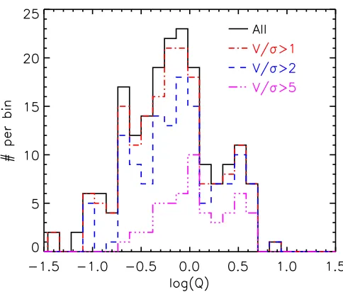
. We also identify a correlation between specific angular momentum and disk stability such that galaxies with the highest specific angular momentum (log(j⋆/ M2⋆/3)>2.5) are the most stable, with
ToomreQ= 1.10±0.18, compared toQ= 0.53±0.22 for galaxies with log(j⋆/ M2⋆/3)<2.5.
At a fixed mass, the HST morphologies of galaxies with the highest specific angular momen-tum resemble spiral galaxies, whilst those with low specific angular momenmomen-tum are morpho-logically complex and dominated by several bright star-forming regions. This suggests that angular momentum plays a major role in defining the stability of gas disks: atz∼1, massive galaxies that have disks with low specific angular momentum, are globally unstable, clumpy and turbulent systems. In contrast, galaxies with high specific angular have evolved in to stable disks with spiral structure where star formation is a local (rather than global) process.
1 INTRODUCTION
Identifying the dominant physical processes that were responsi-ble for the formation of the Hubresponsi-ble sequence has been one of the major goals of galaxy formation for decades (Roberts 1963; Gallagher & Hunter 1984; Sandage 1986). Morphological surveys of high-redshift galaxies, in particular utilizing the high angular resolution of the Hubble Space Telescope; (HST) have suggested that only atz∼1.5 did the Hubble sequence begin to emerge (e.g. Bell et al. 2004; Conselice et al. 2011), with the spirals and ellipti-cals becoming as common as peculiar galaxies (e.g. Buitrago et al. 2013; Mortlock et al. 2013). However, galaxy morphologies reflect the complex (non-linear) processes of gas accretion, baryonic dissi-pation, star formation and morphological transformation that have occured during the history of the galaxy. Furthermore, morpholog-ical studies of high-redshift galaxies are subject to K-corrections and structured dust obscuration, which complicates their interpre-tation.
The more fundamental physical properties of galaxies are their mass, energy and angular momentum, since these are related to the amount of material in a galaxy, the linear size and the rotational ve-locity. As originally suggested by Sandage et al. (1970), the Hub-ble sequence of galaxy morphologies appears to follow a sequence of increasing angular momentum at a fixed mass (e.g. Fall 1983; Fall & Romanowsky 2013; Obreschkow & Glazebrook 2014). One route to identifying the processes responsible for the formation of disks is therefore to measure the evolution of the mass, size and dy-namics (and hence angular momentum) of galaxy disks with cos-mic time – properties which are more closely related to the under-lying dark matter halo.
In the cold dark matter paradigm, baryonic disks form at the centers of dark matter halos. As dark matter halos grow early in their formation history, they acquire angular momentum (J) as a result of large scale tidal torques. The angular momentum acquired has strong mass dependence, with J ∝ Mhalo5/3 (e.g. Catelan & Theuns 1996). Although the halos acquire angular mo-mentum, the centrifugal support of the baryons and dark mat-ter within the virial radius is small. Indeed, whether calculated through linear theory or viaN-body simulations, the “spin” (which defines the ratio of the halo angular speed to that required for the halo to be entirely centrifugally supported) follows approxi-mately a log-normal distribution with average valueλDM= 0.035
(Bett et al. 2007). This quantity is invariant to cosmological param-eters, time, mass or environment (e.g. Barnes & Efstathiou 1987; Steinmetz & Bartelmann 1995; Cole & Lacey 1996).
As the gas collapses within the halo, the baryons can both lose and gain angular momentum between the virial radius and disk scale. If the baryons are dynamically cold, they fall inwards, weakly conserving specific angular momentum. Although the spin of the baryon at the virial radius is small, by the time they reach∼2– 10 kpc (the “size” of a disk), they form a centrifugally supported disk which follows an exponential mass profile (e.g. Fall 1983; Mo et al. 1998). Here, “weakly conserved” is within a factor of two, and indeed, observational studies suggest that late-type spiral disks have a spin ofλ′
disk= 0.025; (e.g. Courteau 1997), suggesting that
that that only∼30% of the initial baryonic angular momentum is lost due to viscous angular momentum redistribution and selective gas losses which occurs as the galaxy disks forms (e.g. Burkert 2009).
In contrast, if the baryons do not make it in to the disk, are redistributed (e.g. due to mergers), or blown out of the galaxy due to winds, then the spin of the disk is much lower than that of the halo.
Indeed, the fraction of the initial halo angular momentum that is lost must be as high as∼90% for early-type and elliptical galaxies (at the same stellar mass as spirals; Bertola & Capaccioli 1975), with Sa and S0 galaxies in between the extremes of late-type spiral-and elliptical- galaxies (e.g. Romanowsky & Fall 2012).
Numerical models have suggested that most of the angu-lar momentum transfer occurs at epochs ealier than z ∼ 1, after which the baryonic disks gain sufficient angular momen-tum to stabilise themselves (Dekel et al. 2009; Ceverino et al. 2010; Obreschkow et al. 2015; Lagos et al. 2016). For example, Danovich et al. (2015) use identify four dominant phases of an-gular momentum exchange that dominate this process: linear tidal torques on the gas beyond and through the virial radius; angular momentum transport through the halo; and dissipation and disk in-stabilities, outflows in the disk itself. These processes can increase and decrease the specific angular momentum of the disk as it forms, although they eventually “conspire” to produce disks that have a similar spin distribution as the parent dark matter halo.
Measuring the processes that control the internal redistribu-tion of angular momentum in high-redshift disks is observaredistribu-tionally demanding. However, on galaxy scales (i.e.∼2–10 kpc), observa-tions suggest redshift evolution according toj⋆= J⋆/ M⋆∝(1+z)n withn∼ −1.5, at least out toz∼2 (e.g. Obreschkow et al. 2015; Burkert et al. 2015). Recently, Burkert et al. (2015) exploited the
KMOS3Dsurvey ofz ∼1–2.5 star-forming galaxies at to infer the angular momentum distribution of baryonic disks, finding that their spin is is broadly consistent the dark matter halos, withλ∼0.037 with a dispersion (σlogλ∼0.2). The lack of correlation between the “spin” (jdisk/jDM) and the stellar densities of high-redshift
galax-ies also suggests that the redistribution of the angular momentum within the disks is the dominant process that leads to compactation (i.e. bulge formation; Burkert et al. 2016; Tadaki et al. 2016). Taken together, these results suggest that angular momentum in high red-shift disks plays a dominant role in “crystalising” the Hubble se-quence of galaxy morphologies.
In this paper, we investigate how the angular momentum and spin of baryonic disks evolves with redshift by measuring the dy-namics of a large, representative sample of star-forming galaxies betweenz ∼0.28–1.65 as observed with the KMOS and MUSE integral field spectrographs. We aim to measure the angular mo-mentum of the stars and gas in large and representative samples of high-redshift galaxies. Only now, with the capabilities of sensitive, multi-deployable (or wide-area) integral field spectrographs, such as MUSE and KMOS, is this becoming possible (e.g. Bacon et al. 2015; Wisnioski et al. 2015; Stott et al. 2016; Burkert et al. 2015). We use our data to investigate how the mass, size, rotational veloc-ity of galaxy disks evolves with cosmic time. As well as providing constraints on the processes which shape the Hubble sequence, the evolution of the angular momentum and stellar mass provides a novel approach to test galaxy formation models since these values reflect the initial conditions of their host halos, merging, and the prescriptions that describe the processes of gas accretion, star for-mation and feedback, all of which can strongly effect the angular momentum of the baryonic disk.
In§2 we describe the observations and data reduction. In§3 we describe the analysis used to derive stellar masses, galaxy sizes, inclinations, and dynamical properties. In§4 we combine the stel-lar masses, sizes and dynamics to measure the redshift evolution of the angular momentum of galaxies. We also compare our re-sults to hydro-dynamical simulations. In§5 we give our conclu-sions. Throughout the paper, we use a cosmology withΩΛ= 0.73,
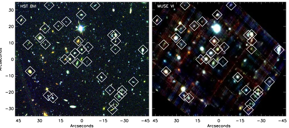
spa-Figure 1.HSTand MUSE images for one of our survey fields, TN J1338−13 which contains az= 4.4 radio galaxy – underlining the fact that our survey of the foreground galaxy population is unbiased. Left:HST BV I-band colour image. The [OII] emitters identified from this field are also marked by open symbols. Center: MUSEV I-band colour image of the cube generated from three equal wavelength ranges. The [OII] emitters are again marked. Each image is centered with (0,0) atα: 13 38 26.1,δ:−19 42 30.5 with North up and East left.
tial resolution of 0.7′′
corresponds to a physical scale of 5.2 kpc at
z= 0.84 (the median redshift of our survey). All quoted magnitudes are on the AB system and we adopt a Chabrier IMF throughout.
2 OBSERVATIONS AND DATA REDUCTION
The observations for this program were acquired from a se-ries of programs (commissioning, guaranteed time and open-time projects; see Table 1) with the new Multi-Unit Spectroscopic Ex-plorer (MUSE; Bacon et al. 2010, 2015) andK-band Multi-Object Spectrograph (KMOS; Sharples et al. 2004) on the ESO Very Large Telescope (VLT). Here, we describe the observations and data re-duction, and discuss how the properties (star-formation rates and stellar masses) of the galaxies in our sample compare to the “main-sequence” population.
2.1 MUSE Observations
As part of the commissioning and science verification of the MUSE spectrograph, observations of fifteen “extra-galactic” fields were taken between 2014 February and 2015 February. The science targets of these programs include “blank” field studies (e.g. ob-servations of the Hubble Ultra-Deep Field; Bacon et al. 2015), as well as high-redshift (z >2) galaxies, quasars and galaxy clus-ters (e.g. Fig. 1) (see also Husband et al. 2015; Richard et al. 2015; Contini et al. 2015). The wavelength coverage of MUSE (4770– 9300 ˚A in its standard configuration) allows us to serendipitously identify [OII] emitters betweenz ∼0.3–1.5 in these fields and so to study the dynamics of star-forming galaxies over this redshift range. We exploit these observation to construct a sample of star-forming galaxies, selected via their [OII] emission. The program IDs, pointing centers, exposure times, seeing FWHM (as measured from stars in the continuum images) for all of the MUSE pointings
are given in Table 1. We also supplement these data with [OII] emit-ters from MUSE observations from two open-time projects (both of whose primary science goals are also to detect and resolve the prop-erties ofz >3 galaxies/QSOs; Table 1). The median exposure time for each of these fields is 12 ks, but ranges from 5.4–107.5 ks. In total, the MUSE survey area exploited here is∼20 arcmin2with a total integration time of 89 hours.
The MUSE IFU provides full spectral coverage spanning 4770–9300 ˚A and a contiguous field of view of 60′′
×60′′
, with a spatial sampling of 0.2′′
/ pixel and a spectral resolution of
R=λ/∆λ= 3500 at λ= 7000 ˚A (the wavelength of the [OII] at the median redshift of our sample) – sufficient to resolve the [OII]λλ3726.2,3728.9 emission line doublet. In all cases, each 1 hour observing block was split in to a number of sub-exposures (typically 600, 1200, or 1800 seconds) with small (2′′
) dithers be-tween exposures to account for bad pixels. All observations were carried out in dark time, good sky transparency. The averageV -band seeing for the observations was 0.7′′
(Table 1).
To reduce the data, we use the MUSEESOREXpipeline which extracts, wavelength calibrates, flat-fields the spectra and forms each datacube. In all of the data taken after August 2014, each 1 hr science observation was interspersed with a flat-field to improve the slice-by-slice flat field (illumination) effects. Sky subtraction was performed on each sub-exposure by identifying and subtract-ing the sky emission ussubtract-ing blank areas of sky at each wavelength slice, and the final mosaics were then constructed using an average with a 3-σclip to reject cosmic rays, using point sources in each (wavelength collapsed) image to register the cubes. Flux calibra-tion was carried out using observacalibra-tions of known standard stars at similar airmass and were taken immediately before or after the sci-ence observations. In each case we confirmed the flux calibration by measuring the flux density of stars with known photometry in the MUSE science field.
To identify [OII] emitters in the cubes, we construct and coadd
[image:3.612.46.540.102.321.2]Table 1. Observing logs
Field Name PID RA Dec texp seeing 3-σSB limit
(J2000) (J2000) (ks) (′′)
MUSE:
J0210-0555 060.A-9302 02:10:39.43 −05:56:41.28 9.9 1.08 9.1
J0224-0002 094.A-0141 02:24:35.10 −00:02:16.00 14.4 0.70 11.0
J0958+1202 094.A-0280 09:58:52.34 +12:02:45.00 11.2 0.80 15.2
COSMOS-M1 060.A-9100 10:00:44.26 +02:07:56.91 17.0 0.90 5.3
COSMOS-M2 060.A-9100 10:01:10.57 +02:04:10.60 12.6 1.0 6.3
TNJ1338 060.A-9318 13:38:25.28 −19:42:34.56 32.0 0.75 4.1
J1616+0459 060.A-9323 16:16:36.96 +04:59:34.30 7.0 0.90 7.6
J2031-4037 060.A-9100 20:31:54.52 −40:37:21.62 37.7 0.83 5.2
J2033-4723 060.A-9306 20:33:42.23 −47:23:43.69 7.9 0.85 7.4
J2102-3535 060.A-9331 21:02:44.97 −35:53:09.31 11.9 1.00 6.2
J2132-3353 060.A-9334 21:32:38.97 −33:53:01.72 6.5 0.70 13.6
J2139-0824 060.A-9325 21:39:11.86 −38:24:26.14 7.4 0.80 5.7
J2217+1417 060.A-9326 22:17:20.89 +14:17:57.01 8.1 0.80 4.9
J2217+0012 095.A-0570 22:17:25.01 +00:12:36.50 12.0 0.69 6.0
HDFS-M2 060.A-9338 22:32:52.71 −60:32:07.30 11.2 0.90 7.3
HDFS-M1 060.A-9100 22:32:55.54 −60:33:48.64 107.5 0.80 2.8
J2329-0301 060.A-9321 23:29:08.27 −03:01:58.80 5.7 0.80 5.6
KMOS:
COSMOS-K1 095.A-0748 09:59:33.54 +02:18:00.43 16.2 0.70 22.5
SSA22 060.A-9460 22:19:30.45 +00:38:53.34 7.2 0.72 31.2
SSA22 060.A-9460 22:19:41.15 +00:23:16.65 7.2 0.70 33.7
Notes: RA and Dec denote the field centers. The seeing is measured from stars in the field of view (MUSE) or from a star placed on one of the IFUs (KMOS). The units of the surface brightness limit are×10−19erg s−1cm−2arcsec−2. The reduced MUSE datacubes for these fields available at:
http://astro.dur.ac.uk/∼ams/MUSEcubes/
cubes over the wavelength rangesλ= 4770–7050 ˚A andλ= 7050– 9300 ˚A respectively. We then useSEXTRACTOR(Bertin & Arnouts 1996) to identify all of the>4σ continuum sources in the “de-tection” images. For each continuum source, we extract a 5×5′′ sub-cube (centered on each continuum source) and search both the one and two-dimensional spectra for emission lines. At this res-olution, the [OII] doublet is resolved and so trivially differenti-ated from other emission lines, such as Lyα, [OIII] 4959,5007 or Hα+[NII] 6548,6583. In cases where an emission line is identified, we measure the wavelength,x/y(pixel) position and RA / Dec of the galaxy. Since we are interested in resolved dynamics, we only include galaxies where the [OII] emission line is detected above 5σin the one dimensional spectrum. To ensure we do not miss any [OII] emitters that do not have continuum counterparts, we also re-move all of the continuum sources from each cube by masking a 5′′ diameter region centered on the continuum counterpart, and search the remaining cube for [OII] emitters. We do not find any additional [OII]-emitting galaxies where the integrated [OII] flux is detected above a signal-to-noise of 5 (i.e. all of the bright [OII] emitters in our sample have at least a 4σdetection in continuum).
In Fig. 1 we show a HSTBV I-band colour image of one of our target fields, TNJ 1338, along with a colour image generated from the 32 ks MUSE exposure. The blue, green and red channels are generated from equal width wavelength ranges between 4770– 9300 AA in the MUSE cube. In both panels we identify all of the [OII] emitters. In this single field alone, there are 33 resolved [OII] emitters.
From all 17 MUSE fields considered in this analysis, we iden-tify a total of 431 [OII] emitters with emission line fluxes
rang-ing from 0.1–170×10−17erg s−1cm−2 with a median flux of
3×10⁻¹⁷erg s−1cm−2and a median redshift ofz= 0.84 (Fig. 2).
Before discussing the resolved properties of these galaxies, we first test how our [OII]-selected sample compares to other [OII] surveys at similar redshifts. We calculate the [OII] lumi-nosity of each galaxy and in Fig. 2 show the [OII] luminosity function in two redshift bins (z= 0.3–0.8 and z= 0.8–1.4). In both redshift bins, we account for the incompleteness caused by the exposure time differences between fields. We highlight the luminosity limits for four of the fields which span the whole range of depths in our survey. This figure shows that the [OII] luminosity function evolves strongly with redshift, with
L⋆ evolving from log
10(L⋆[erg s−1cm−2]) = 41.06±0.17
at z= 0 to log10(L⋆[erg s−1cm−2]) = 41.5±0.20 and
log10(L⋆[erg s−1cm−2]) = 41.7±0.22 at z= 1.4 (see also
Ly et al. 2007; Khostovan et al. 2015). The same evolution has also been seen in at UV wavelengths (Oesch et al. 2010) and in Hαemission (e.g. Sobral et al. 2013a).
2.2 KMOS Observations
Figure 2. Left: [OII] luminosity function for the star-forming galaxies in our sample from the 18 MUSE IFU pointings. We split the sample in two redshift bins,z= 0.3–0.8 andz= 0.8–1.4. The arrows on the plot denote luminosity limits for four of the fields in the MUSE sample (which span the complete range of depths). To baseline these results, we overlay the [OII] luminosity function atz= 0 from SDSS (Ciardullo et al. 2013) which shows that there is strong evolution in L⋆
[OII]fromz∼0 toz∼0.5. This evolution is also seen in other [OII] surveys (e.g. Ly et al. 2007; Khostovan et al. 2015). Right: The redshift
distribution of the [OII] and Hαemitters in our MUSE and KMOS samples. Our sample has a median redshift ofz= 0.84 and a full redshift range ofz= 0.28– 1.67. Since the MUSE observations have a wide range of exposure times, from 5.7–107.5 ks, we overlay the redshift distribution of the [OII] emitters in the two deepest fields, HDFS and TNJ 1338, to highlight that the highest-redshift galaxies are not dominated by the deepest observations. We also overlay the redshift distribution of the galaxies classified as “rotationally supported” (i.e. disks).
24 IFUs, each of size 2.8×2.8′′
sampled at 0.2′′
which can be de-ployed across a 7-arcmin diameter patrol field. The total exposure time was 7.2 ks per pixel, and we used object-sky-object observing sequences, with one IFU from each of the three KMOS spectro-graphs placed on sky to monitor OH variations.
Further KMOS observations were also obtained between 2015 April 25 and April 27 as the first part of a 20-night KMOS guaranteed time programme aimed at resolving the dynamics of 300 mass-selected galaxies at z ∼1.2–1.7. Seventeen galaxies were selected from photometric catalogs of the COSMOS field. We initially selected targets in the redshift rangez= 1.3–1.7 and brighter thanKAB= 22 (a limit designed to ensure we obtain
suf-ficient signal-to-noise per resolution element to spatially resolve the galaxies; see Stott et al. 2016 for details). To ensure that the Hαemission is bright enough to detect and spatially resolve with KMOS, we pre-screened the targets using the Magellan
Multi-object Infra-Red Spectrograph (MMIRS) to search for and mea-sure the Hαflux of each target, and then carried out follow-up observations with KMOS of those galaxies with Hαfluxes brighter than 5×10⁻¹⁷erg s−1cm−2. These KMOS observations were
car-ried out using theH-band filter, which has a spectral resolution ofR=λ/∆λ= 4000. We used object-sky-object sequences, with one of the IFUs placed on a star to monitor the PSF and one IFU on blank sky to measure OH variations. The total exposure time was 16.2 ks (split in to three 5.4 ks OBs, with 600 s sub-exposures). Data reduction was performed using theSPARKpipeline with addi-tional sky-subtraction and mosaicing carried out using customized routines. We note that a similar dymamical / angular momemtum analysis of the∼800 galaxies atz∼1 from the KROSS survey are presented in Harrison et al. (2017).
2.3 Final Sample
Combining the two KMOS samples, in total there are 41 / 46 Hα -emitting galaxies suitable for this analysis (i.e. Hαdetected above a S / N>5 in the collapsed, one-dimensional spectrum). From our MUSE sample of 431 galaxies, 67 of the faintest [OII] emitters are only detected above a S / N = 5 when integrating a 1×1′′region, and so no longer considered in the following analysis, leaving us with a sample of 364 [OII] emitters for which we can measure re-solved dynamics. Together, the MUSE and KMOS sample used in the following analysis comprises 405 galaxies with a redshift range
z= 0.28–1.63. We show the redshift distribution for the full sample in Fig. 2.
3 ANALYSIS
With the sample of 405 emission-line galaxies in our survey fields, the first step is to characterize the integrated properties of the galax-ies. In the following, we investigate the spectral energy distribu-tions, stellar masses and star formation rates, sizes, dynamics, and their connection with the galaxy morphology, and we put our find-ings in the context of our knowledge of the general galaxy popula-tion at these redshifts. We first discuss their stellar masses.
3.1 Spectral Energy Distributions and Stellar Masses
imag-ing. In the optical / near-infrared imaging, we measure 2′′ aper-ture photometry, whilst in the IRAC 3.6 / 4.5-µm bands we use 5′′ apertures (and apply appropriate aperture corrections based on the PSF in each case). We list all of the properties for each galaxy, and show their broad-band SEDs in Table A1. We use HYPER
-z (Bol-zonella et al. 2000) to fit the photometry of each galaxy
at the known redshift, allowing a range of star formation histo-ries from late to early types and redennings of AV= 0–3 in steps
of∆AV= 0.2 and a Calzetti dust reddening curve (Calzetti et al.
2000). In cases of non detections, we adopt a 3σupper limit. We show the observed photometry and overlay the best-fit
HYPER-z SED for all of the galaxies in our sample in Fig. A1– A3. Using the best-fit parameters, we then estimate the stellar mass of each galaxy by integrating the best-fit star-formation history, ac-counting for mass loss according to theSTARBURST99 mass loss rates (Leitherer et al. 1999). We note that we only calculate stellar masses for galaxies that have detections in>3 wavebands, although include the best SEDs for all sources in Fig. A1–A3. Using the stel-lar masses and rest-frameH-band magnitudes, we derive a median mass-to-light ratio for the full sample of M⋆/ LH= 0.20±0.01. The
best-fit reddening values and the stellar masses for each galaxy are also given in Table A1.
As a consistency check that our derived stellar masses are con-sistent with those derived from other SED fitting codes, we com-pare our results with Muzzin et al. (2013) who derive the stellar masses of galaxies in the COSMOS field using theEASY photomet-ric redshift code (Brammer et al. 2008) with stellar mass estimated usingFASTKriek et al. (2009). For the 54 [OII] emitting galaxies in the COSMOS field in our sample, the stellar masses we derive are a factor 1.19±0.06×higher than those derived usingFAST. Most of this difference can be attributed to degeneracies in the redshifts and best-fit star-formation histories. Indeed, if we limit the compar-ison to galaxies where the photometric and spectroscopic redshifts agree within∆z <0.2, and where the luminosity weighted ages also agrees to within a factor of 1.5, then then the ratio of the stel-lar masses fromHYPER-Z/EASYare 1.02±0.04×.
To place the galaxies we have identified in the MUSE and KMOS data in context of the general population at their respective redshifts, next we calculate their star formation rates (and specific star formation rates). We first calculate the [OII] or Hαemission lu-minosity (L[OII]and LHαrespectively). To account for dust obscu-ration, we adopt the best-fit stellar redenning (AV) from the stellar
SED returned by fromHYPER-Zand convert this to the attenua-tion at the wavelength of interest (A[OII]or AHα) using a Calzetti
reddennign law; Calzetti et al. 2000). Next, we assume that the the gas and stellar phases are related by Agas= A⋆(1.9−0.15 A⋆);
(Wuyts et al. 2013), and then calculate the total star-formation rates using SFR =C×10−42L
[OII]100.4Agas with C= 0.82 and
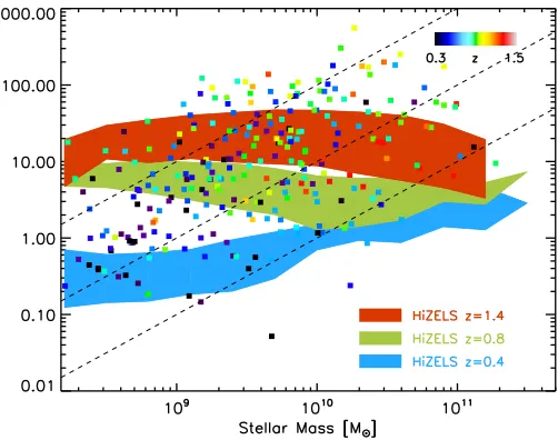
[image:6.612.304.555.100.298.2]C= 4.6 for the [OII] and Hαemitters respectively. The star for-mation rates of the galaxies in our sample range from 0.1– 300 M⊙yr−1. In Fig. 3 we plot the specific star-formation rate (sSFR = SFR / M⋆) versus stellar mass for the galaxies in our sam-ple. This also shows that our sample display a wide range of stellar masses and star-formation rates, with median and quartile ranges of log10(M⋆/ M⊙) = 9.4±0.9 and SFR = 4.7+2−2..25M⊙yr−1. As a guide, in this plot we also overlay a track of constant star forma-tion rate with SFR = 1 M⊙yr−1. To compare our galaxies to the high-redshift star-forming population, we also overlay the specific star formation rate for∼2500 galaxies from the HiZELS survey which selects Hαemitting galaxies in three narrow redshifts slices atz= 0.40, 0.84 and 1.47 (Sobral et al. 2013a). For this compari-son, we calculate the star formation rates for the HiZELS galaxies
Figure 3. Star-formation rate versus mass for the galaxies in our sample (with points colour-coded by redshift). As a guide, we also overlay tracks of constant specific star formation rate (sSFR) with with sSFR = 0.1, 1 and 10 Gyr−1. We also overlay the star formation rate–stellar mass relation at three
redshift slices (z= 0.40, 0.84 and 1.47) from the Hαnarrow-band selected sample from HiZELS (Sobral et al. 2013a). This shows that although the galaxies in our MUSE and KMOS samples span a wide range of stellar mass and star-formation rate, they are comparable to the general field population, with specific star formation rates sSFR∼0.1–10 Gyr−1.
in an identical manner to that for our MUSE and KMOS sample. This figure shows that the median specific star formation rate of the galaxies in our MUSE and KMOS samples appear to be consis-tent with the so-called “main-sequence” of star-forming galaxies at their appropriate redshifts.
3.2 Galaxy Sizes and Size Evolution
Next, we turn to the sizes for the galaxies in our sample. Studies of galaxy morphology and size, particularly from observations made with HST, have shown that the physical sizes of galaxies increase with cosmic time (e.g. Giavalisco et al. 1996; Ferguson et al. 2004; Oesch et al. 2010). Indeed, late-type galaxies have contin-uum (stellar) half light radii that are on average a factor∼1.5×
smaller atz ∼1 than at the present day (van der Wel et al. 2014; Morishita et al. 2014). As one of the primary aims of this study is to investigate the angular momentum of the galaxy disks, the con-tinuum sizes are an important quantity.
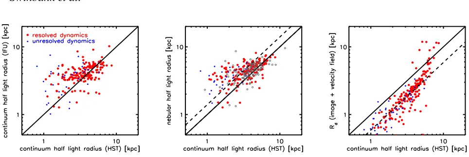
the PSF). In Fig. 4 we compare the half-light radius of the galax-ies in our sample from HST observations with that measured from the MUSE and KMOS continuum images. From this, we derive a median ratio ofr1/2,HST/r1/2,MUSE= 0.97±0.03 with a scatter
of 30% (including unresolved sources in both cases).
For each galaxy in our sample, we also construct a continuum-subtracted narrow-band [OII] or Hαemission line image (using 200 ˚A on either size of the emission line to define the continuum) and use the same technique to measure the half-light radius of the nebular emission. The continuum and nebular emission line half light radii (and their errors) for each galaxy are given in Table A1. As Fig. 4 shows, the nebular emission is more extended that the continuum withr1/2,[OII]/r1/2,HST= 1.18±0.03. This is
consis-tent with recent results from the 3-D HST survey demonstrates that the nebular emission from∼L⋆galaxies atz ∼1 tends to be sys-tematically more extended than the stellar continuum (with weak dependence on mass; Nelson et al. 2015).
We also compare the continuum half light radius with the disk scale length, Rd (see§ 3.4). From the data, we measure a
r1/2,HST/Rd= 1.70±0.05. For a galaxy with an exponential light
profile, the half light radii and disk scale length are related by
r1/2= 1.68Rd, which is consistent with our measurements (and we
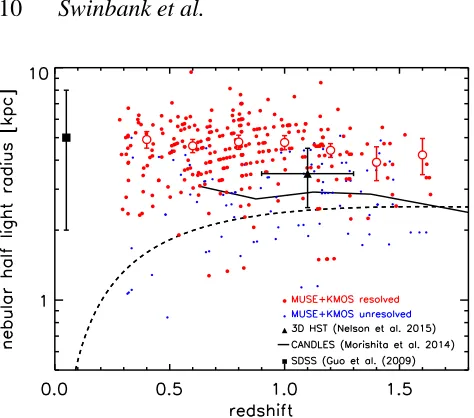
overlay this relation in Fig. 4). In Fig. 6 we plot the evolution of the half-light radii (in kpc) of the nebular emission with redshift for the galaxies in our sample which shows that the nebular emission half-light radii are consistent with similar recent measurements of galaxy sizes from HST (Nelson et al. 2015), and a factor∼1.5×
smaller than late-type galaxies atz= 0.
From the full sample of [OII] or Hαemitters, the spatial extent of the nebular emission of 75% of the sample are spatially resolved beyond the seeing, with little / no dependence on redshift, although the unresolved sources unsurprisingly tend to have lower stel-lar masses (median Munresolved⋆ = 1.0±0.5×10⁹M⊙compared to median Mresolved⋆ = 3±1×10⁹M⊙).
3.3 Resolved Dynamics
Next, we derive the velocity fields and line-of-sight velocity dis-persion maps for the galaxies in our sample. The two-dimensional dynamics are critical for our analysis since the circular velocity, which we will use to determine the angular momentum in§4, must be taken from the rotation curve at a scale radius. The observed circular velocity of the galaxy also depends on the disk inclination, which can be determined using either the imaging, or dynamics, or both.
To create intensity, velocity and velocity dispersion maps for each galaxy in our MUSE sample, we first extract a 5×5′′ “sub-cube” around each galaxy (this is increased to 7×7′′
if the [OII] is very extended) and then fit the [OII] emission line doublet pixel-by-pixel. We first average over 0.6×0.6′′
pixels and attempt the fit to the continuum plus emission lines. During the fitting proce-dure, we account for the increased noise around the sky OH resid-uals, and also account for the the spectral resolution (and spectral line spread function) when deriving the line width. We only accept the fit if the improvement over a continuum-only fit is>5σ. If no fit is achieved, the region size is increased to 0.8×0.8′′and the fit re-attempted. In each case, the continuum level, redshift, line width, and intensity ratio of the 3726.2 / 3728.9 ˚A [OII] emission line doublet is allowed to vary. In cases that meet the signal-to-noise threshold, errors are calculated by perturbing each parameter in turn, allowing the other parameters to find their new minimum, until a∆χ2= 1-σis reached. For the KMOS observations we
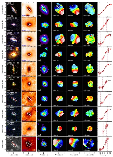
fol-low the same procedure, but fit the Hαand [NII] 6548,6583 emis-sion lines. In Fig. 5 we show example images and velocity fields for the galaxies in our sample (the full sample, along with their spectra are shown in Appendix A). In Fig. 5 the first three panels show the
HST image, with ellipses denoting the disk radius and lines
identi-fying the major morphological and kinematic axis (see§3.4), the MUSEI-band continuum image and the two-dimensional velocity field. We note that for each galaxy, the high-resolution image (usu-ally from HST) is astrometric(usu-ally aligned to the MUSE or KMOS cube by cross correlating the (line free) continuum image from the cube.
The ratio of circular velocity (or maximum velocity if the dy-namics are not regular) to line-of-sight velocity dispersion (V /σ) provides a crude, but common way to classify the dynamics of galaxies in to rotationally- version dispersion- dominated systems. To estimate the maximum circular velocity,V, we extract the ve-locity profile through the continuum center at a position angle that maximises the velocity gradient. We inclination correct this value using the continuum axis ratio from the broad-band contin-uum morphology (see§3.4). For the full sample, we find a range of maximum velocity gradients from 10 to 540 km s−1
(peak-to-peak) with a median of 98±5 km s−1and a quartile range of 48–
192 km s−1. To estimate the intrinsic velocity dispersion, we first
remove the effects of beam-smearing (an effect in which the ob-served velocity dispersion in a pixel has a contribution from the intrinsic dispersion and the flux-weighted velocity gradient across that pixel due to the PSF). To derive the intrinsic velocity disper-sion, we calculate and subtract the luminosity weighted velocity gradient across each pixel and then calculate the average veloc-ity dispersion from the corrected two-dimensional velocveloc-ity dis-persion map. In this calculation, we omit pixels that lie within the central PSF FWHM (typically ∼0.6′′
; since this is the re-gion of the galaxy where the beam-smearing correction is most uncertain). For our sample, the average (corrected) line-of-sight velocity dispersion isσ= 32±4 km s−1 (in comparison, the
aver-age velocity dispersion measured from the galaxy integrated one-dimensional spectrum isσ= 70±5 km s−1). This average intrinsic
velocity dispersion at the median redshift of our sample (z= 0.84) is consistent with the average velocity dispersion seen in a num-ber of other high-redshift samples (e.g. F¨orster Schreiber et al. 2009; Law et al. 2009; Gnerucci et al. 2011; Epinat et al. 2012; Wisnioski et al. 2015).
For the full sample of galaxies in our survey, we derive a me-dian inclination corrected ratio ofV /σ= 2.2±0.2 with a range of
V/σ= 0.1–10 (where we use the limits on the circular velocities for galaxies classed as unresolved or irregular / face-on). We show the full distribution in Fig. 7.
Although the ratio ofV/σprovides a means to separate “ro-tationally dominated” galaxies from those that are dispersion sup-ported, interacting or merging can also be classed as rotationally supported. Based on the two-dimensional velocity field, morphol-ogy and velocity dispersion maps, we also provide a classification of each galaxy in four broad groups (although in the following dy-namical plots, we highlight the galaxies byV /σand their classifi-cation):
(i) Rotationally supported: for those galaxies whose dynamics
Figure 4. Comparison of the physical half-light radii of the galaxies in our sample as measured from HST and MUSE / KMOS imaging. Left: Continuum half-light radii as measured from HST broad-band imaging compared to those measured from the MUSE continuum image. Large red points denote sources that are resolved by MUSE or KMOS. Small blue point denote galaxies that are unresolved (or compact) in the MUSE or KMOS data. The median ratio of the half-light radii isrHST/rMUSE= 0.97±0.03 (including unresolved sources and deconvolved for seeing). Center: Continuum half-light radius from
HST versus nebular emission half-light radius (MUSE and KMOS) for the galaxies in our sample from MUSE and KMOS. The continuum and nebular emission line half-light radii are well correlated, although the nebular emission lines half-light radii are systematically larger than the continuum sizes, with r[OII]/rHST= 1.18±0.03 (see also Nelson et al. 2015). Although not included in the fit, we also include on the plot the contuinuum size measurements from
MUSE and KMOS as small grey points. These increase the scatter (as expected from the data in the left-hand panel), although the median ratio of nebular emission to continuum size is unaffected if these points are included. Right: Comparison of the disk scale length (measured from the dynamical modeling) versus the continuum half-light radius from HST. The median ratio of the half-light radius is larger than the disk radius by a factorrHST/Rd= 1.70±0.05,
which is the consistent with that expected for an exponential disk.
and those whose rotation curves do not appear to have asymptoted at the maximum radius determined by the data (q= 2). This pro-vides an important distinction since for a number ofq= 2 cases the asymptotic rotation speed must be extrapolated (see§3.6). The im-ages, spectra, dynamics and broad-band SEDs for these galaxies are shown in Fig. A1.
(ii) Irregular: A number of galaxies are clearly resolved beyond the
seeing, but display complex velocity fields and morphologies, and so we classify as “Irregular”. In many of these cases, the morphol-ogy appears disturbed (possibly late stage minor / major mergers) and / or we appear to be observing systems (close-to) face-on (i.e. the system is spatially extended by there is little / no velocity struc-ture discernable above the errors). The images, spectra, dynamics and broad-band SEDs for these galaxies are shown in Fig. A2.
(iii) Unresolved: As discussed in§3.2, the nebular emission in a significant fraction of our sample appear unresolved (or “compact”) at our spatial resolution. The images, spectra, dynamics and broad-band SEDs for these galaxies are shown in Fig. A3.
(iv) Major Mergers: Finally, a number of systems appear to
com-prise of two (or more) interacting galaxies on scales separated by 8–30 kpc, and we classify these as (early stage) major mergers. The images, spectra, dynamics and broad-band SEDs for these galaxies are shown in Fig. A2.
From this broad classification, our [OII] and Hα selected sample comprises 24±3% unresolved systems; 49±4% rotation-ally supported systems (27% and 21% with q= 1 and q= 2 re-spectively); 22±2% irregular (or face-on) and ∼5±2% major mergers. Our estimate of the “disk” fraction in this sample is consistent with other dynamical studies over a similar redshift range which found that rotationally supported systems make up
∼40–70% of the Hα- or [OII]-selected star-forming population (e.g. F¨orster Schreiber et al. 2009; Puech et al. 2008; Epinat et al. 2012; Sobral et al. 2013b; Wisnioski et al. 2015; Stott et al. 2016; Contini et al. 2015).
From this classification, the “rotationally supported” systems are (unsurprisingly) dominated by galaxies with highV/σ, with
176/195 (90%) of the galaxies classed as rotationally supoprted with V/σ > 1(and 132 / 195 [67%] with V /σ >2). Concentrat-ing only on those galaxies that are classified as rotationally sup-ported systems (§3.3), we deriveV/σ= 2.9±0.2 [3.4±0.2 and 1.9±0.2 for theq= 1 andq= 2 sub-samples respectively]. We note that 23% of the galaxies that are classified as rotationally supported haveV/σ <1(21% withq= 1 and 24% withq= 2).
3.4 Dynamical Modeling
For each galaxy, we model the broad-band continuum image and two-dimensional velocity field with a disk + halo model. In addi-tion to the stellar and gaseous disks, the rotaaddi-tion curves of local spiral galaxies imply the presence of a dark matter halo, and so the velocity field can be characterized by
v2 = vd2 +vh2 + vHI2
where the subscripts denote the contribution of the baryonic disk (stars + H2), dark halo and extended HIgas disk respectively. For the disk, we assume that the baryonic surface mass density follows an exponential profile (Freeman 1970)
Σd(r) = Md
2πR2 d
e−r/Rd
whereMdandRdare the disk mass and disk scale length
respec-tively. The contribution of this disk to the circular velocity is:
v2D(x) =
1 2
GMd
Rd
(3.2x)2(I0K0−I1K1)
wherex=R/RdandInandKnare the modified Bessel functions
computed at 1.6x. For the dark matter component we assume
vh2(r) = GMh(< r)/ r
with
ρ(r) = ρ0r
3 0
Figure 5. Example images and dynamics of nine galaxies in our sample. (a): HST colour image of each galaxy. given in each sub-image. The galaxies are ranked by increasing redshift. The ellipses denote the disk radius (inner ellipse Rd; outer ellipse 3 Rd). The cross denotes the dynamical center of the galaxy
and the white-dashed and solid red line show the major morphological and kinematic axes respectively. (b): The continuum image from the IFU observations (dark scale denotes high intensity). The dashed lines are the same as in the first panel. (c): Nebular emission line velocity field. Dashed ellipses again show the disk radius at Rdand 3 Rd(the colour scale is set by the range shown in the final panel). (d): Best-fit two-dimensional dynamical model for each galaxy. In
Figure 6. Evolution of the physical half-light radii with redshift for the galaxies in our sample. We plot the nebular emission line sizes in all cases ([OII] for MUSE or Hαfor KMOS). We plot both the extended (red) and unresolved/compact (blue) galaxies individually, but also show the median half-light radii in∆z= 0.2 bins as large filled points with errors (these me-dians include unresolved sources). We also include recent measurements of the nebular emission line half-light radii ofz∼1 galaxies from the 3D-HST survey (Nelson et al. 2015) and the evolution in the continuum sizes (cor-rected to nebular sizes using the results from Fig 4) from (Morishita et al. 2014) for galaxies in the CANDLES fields. We also include the size mea-surements from SDSS (Guo et al. 2009). As a guide, the dashed line shows the half light radius as a function of redshift for a 0.7′′PSF (the median seeing of our observations). This plot shows that the nebular emission half-light radii of the galaxies in our sample are consistent with similar recent measurements of galaxy sizes from HST (Nelson et al. 2015), and a factor ∼1.5×smaller than late-type galaxies atz= 0.
(Burkert 1995; Persic & Salucci 1988; Salucci & Burkert 2000) wherer0 is the core radius and ρ0 the effective core density. It
follows that
Mh(r) = 4M0
ln1 + r
r0
−tan−1r
r0
+ 1 2 ln
1 +r
2
r2 0
withM0= 1.6ρ0r30and
vH2(r) = 6.4G ρ0r
3 0
r
n
ln
1 + r
r0
−tan−1r
r0
+1 2ln
h
1 +
r
r0
2io
This velocity profile is generic: it allows a distribution with a core of sizer0, converges to the NFW profile (Navarro et al. 1997) at
large distances and, for suitable values ofr0, it can mimic the NFW
or an isothermal profile over the limited region of the galaxy which is mapped by the rotation curve.
In luminous local disk galaxies the HIdisk is the dominant baryonic component forr >3Rd. However, at smaller radii the HI
gas disk is negligible, with the dominant component in stars. Al-though we can not exclude the possibility that some fraction of HI
is distributed within 3Rdand so contributes to the rotation curve, for simplicity, here we assume that the fraction of HIis small and so setvHI= 0.
To fit the the dynamical models to the observed images and velocity fields, we use an MCMC algorithm. We first use the imag-ing data to estimate of the size, position angle and inclination of the galaxy disk. Using the highest-resolution image, we fit the galaxy image with a disk model, treating the [xim,yim] center, position
angle (PAim), disk scale length (Rd) and total flux as free
[image:10.612.303.550.94.366.2]param-eters. We then use the best-fit parameter values from the imaging
Figure 7. The ratio of circular velocity to velocity dispersion for the galax-ies in our sample (V /σ), split by their classification (the lower panel shows the cumulative distribution). The circular velocity has been inclination cor-rected, and the velocity dispersion has been corrected for beam-smearing effects. The dashed line shows all of the galaxies in our sample which are spatially resolved. The red solid line denotes galaxies which are classified as disk-like. The grey box denotes the area occupied by the galaxies that are classified as unresolved. Finally, the dotted line shows a ratio ofV /σ= 1. 90% of the galaxies that are classified as disk-like (i.e. a spider-line pat-tern in the velocity field, the line-of-sight velocity dispersion peaks near the dynamical center of the galaxy and the rotation curve rises smoothly) have V /σ >1, and 67% haveV/σ >2.
as the first set of prior inputs to the code and simultaneously fit the imaging + velocity field using the model described above. For the dynamics, the mass model has five free parameters: the disk mass (Md), radius (Rd), and inclination (i), the core radiusr0, and the
central core densityρ0. We allow the dynamical center of the disk
([xdyn,ydyn]) and position angle (PAdyn) to vary, but require that
the imaging and dynamical center lie within 1 kpc (approximately the radius of a bulge atz ∼1; Bruce et al. 2014). We note also that we allow the morphological and dynamical major axes to be independent (but see§3.5).
To test whether the parameter values returned by the disk mod-eling provide a reasonably description of the data, we perform a number of checks, in particular to test the reliability of recover-ing the dynamical center, position angle and disk inclination (since these propagate directly in to the extraction of the rotation curve and hence our estimate of the angular momentum).
the inclinations, withiin=iout±2◦. Allowing a completely uncon-strained fit returns inclinations which are higher than the input val-ues, (iin/iout= 1.2±0.1), the scatter in which can be attributed to degeneracies with other parameters. For example, the disk masses and disk sizes are over-estimated (compared to the input model), with Mdin/Mdout= 0.86±0.12 and Rind /Routd = 0.81±0.05, but
the position angle of the major axis of the galaxy is recovered to within one degree (PAin−PAout= 0.9±0.7◦). For the purposes of
this paper, since we are primarily interested in identifying the ma-jor kinematic axis (the on-sky position angle), extracting a rotation curve about this axis and correcting for inclination effects, the re-sults of the dynamical modeling appear as sufficiently robust that meaningful measurements can be made.
Next, we test whether the inclinations derived from the mor-phologies alone are comparable to those derived from a simultane-ous fit to the images and galaxy dynamics. To obtain an estimate of the inclination, we useGALFIT(Peng et al. 2002) to model the morphologies for all of the galaxies in our sample which have HST imaging. The ellipticity of the projected image is related to the in-clination angle through cos2i=((b/a)2−q2
0)/(1−q0)2wherea
andbare the semi-major and semi-minor axis respectively (here
iis the inclination angle of the disk plane to the plane of the sky andi= 0 represents an edge-on galaxy). The value ofq0(which
ac-counts for the fact that the disks are not thin) depends on galaxy type, but is typically in the range q0= 0.13–0.20 for rotationally
supported galaxies at z ∼0, and so we adoptq0= 0.13. We first
construct the point-spread function for each HST field using non-saturated stars in the field of view, and then runGALFITwith Sersic index allowed to vary fromn= 0.5–7 and free centers and effec-tive radii. For galaxies whose dynamics resemble rotating systems (such that a reasonable estimate of the inclination can be derived) the inclination derived from the morphology is strongly correlated with that inferred from the dynamics, with a median offset of just
∆i= 4◦
with a spread ofσi= 12◦.
The images, velocity fields, best-fit kinematic maps and ve-locity residuals for each galaxy in our sample are shown in Fig. A1–A3, and the best-fit parameters given in Table A1. Here, the errors reflect the range of acceptable models from all of the models attempted. All galaxies show small-scale devia-tions from the best-fit model, as indicated by the typical r.m.s,
<data−model>= 28±5 km s−1. These offsets could be caused
by the effects of gravitational instability, or simply be due to the un-relaxed dynamical state indicated by the high velocity disper-sions in many cases. The goodness of fit and small-scale deviations from the best-fit models are similar to those seen in other dynam-ical surveys of galaxies at similar redshifts, such as KMOS3Dand KROSS (Wisnioski et al. 2015; Stott et al. 2016) where rotational support is also seen in the majority of the galaxies (and with r.m.s of 10–80 km s−1between the velocity field and best-fit disk mod-els).
3.5 Kinematic versus Morphological Position Angle
One of the free parameters during the modeling is the offset be-tween the major morphological axis and the major dynamical axis. The distribution of misalignments may be attributed to physical differences between the morphology of the stars and gas, extinc-tion differences between the rest-frame UV / optical and Hα, sub-structure (clumps, spiral arms and bars) or simply measurement errors when galaxies are almost face on. Following Franx et al. (1991) (see also Wisnioski et al. 2015), we define the misalign-ment parameter,Φ, such that sinΦ=|sin(PAphot−PAdyn)|where
Φ ranges from 0–90◦. For all of the galaxies in our sample whose dynamics resemble rotationally supported systems, we de-rive a median “misalignment” ofΦ= 9.5±0.5◦
(Φ= 10.1±0.8◦ and 8.6±0.9◦
forq= 1 andq= 2 sub-samples respectively). In all of the following sections, when extracting rotation curves (or veloc-ities from the two-dimensional velocity field), we use the position angle returned from the dynamical modeling, but note that using the morphological position angle instead would reduce the peak-to-peak velocity by<∼5%, although this would have no qualitative effect on our final conclusions.
3.6 Velocity Measurements
To investigate the various velocity–stellar mass and angular mo-mentum scaling relations, we require determination of the cir-cular velocity. For this analysis, we use the best-fit dynamical models for each galaxy to make a number of velocity measure-ments. We measure the velocity at the “optical radius”,V(3Rd)
(Salucci & Burkert 2000) (where the half light- and disk- radius are related byr1/2= 1.68 Rd). Although we are using the
dynam-ical models to derive the velocities (to reduce errors in interpo-lating the rotation curve data points), we note that the average velocity offset between the data and model for the rotationally supported systems at r1/2 is small, ∆V= 2.1±0.5 km s−1 and
∆V = 2.4±1.2 km s−1 at 3R
d. In 30% of the cases, the
veloci-ties at 3Rdare extrapolated beyond the extent of the observable rotation curve, although the difference between the velocity of the last data point on the rotation curve and the velocity at 3Rdin this
sub-sample is only∆v= 2±1 km s−1on average.
3.7 Angular Momentum
With measurements of (inclination corrected) circular velocity, size and stellar mass of the galaxies in our sample, we are in a position to combine these results and so measure the specific angular mo-mentum of the galaxies (measuring the specific angular momo-mentum removes the implicit scaling betweenJand mass). The specific an-gular momentum is given by
j⋆=
J M⋆
=
R
r(r×v¯)ρ⋆d 3r
R
rρ⋆d
3r (1)
whererandv¯(r)are the position and mean-velocity vectors (with respect to the center of mass of the galaxy) andρ(r)is the three dimensional density of the stars and gas.
To enable us to compare our results directly with similar mea-surements atz ∼0, we take the same approximate estimator for specific angular momentum as used in Romanowsky & Fall (2012) (although see Burkert et al. 2015 for a more detailed treatment of angular momentum at high-redshift). In the local samples of Romanowsky & Fall (2012) (see also Obreschkow et al. (2015)), the scaling between specific angular momentum, rotational velocity and disk size for various morphological types is given by
jn=knCivsR1/2 (2)
where vs is the rotation velocity at 2× the half-light radii
(R1/2) (which corresponds to ≃ 3RD for an exponential
disk), Ci= sin−1θim is the deprojection correction factor (see
Romanowsky & Fall 2012) andkndepends on the Sersic index (n)
of the galaxy which can be approximated as
For the galaxies withHST images, we runGALFITto estimate the sersic index for the longest-wavelength image available and de-rive a median sersic index ofn= 0.8±0.2, with 90% of the sam-ple havingn < 2.5, and therefore we adoptj⋆=jn=1, which is
applicable for exponential disks. Adopting a sersic index ofn= 2 would result in a∼20% difference inj⋆. To infer the circular ve-locity, we measure the velocity from the rotation curve at 3Rd; Romanowsky & Fall 2012). We report all of our measurements in Table A1.
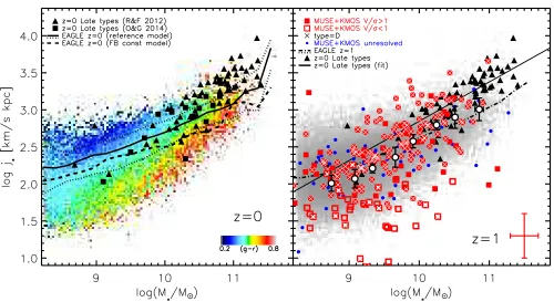
In Fig. 8 we plot the specific angular momentum versus stellar mass for the high-redshift galaxies in our sample and compare to observations of spiral galaxies atz= 0 (Romanowsky & Fall 2012; Obreschkow & Glazebrook 2014). We split the high-redshift sam-ple in to those galaxies with the best samsam-pled dynamics / rotation curves (q= 1) and those with less well constrained dynamics (q= 2). To ensure we are not biased towards large / resolved galax-ies in the high-redshift sample, we also include the unresolved galaxies, but approximate their maximum specific angular momen-tum by j⋆= 1.3r1/2σ (where σ is the velocity dispersion
mea-sured from the collapsed, one-dimensional spectrum and is as-sumed to provide an upper limit on the circular velocity. The pre-factor of 1.3 is derived assuming a Sersic index ofn= 1–2; Romanowsky & Fall 2012). We note that three of our survey fields (PKS1614−9323, Q2059−360 and Q0956+122) do not have ex-tensive multi-wavelength imaging required to derive stellar masses and so do not include these galaxies on the plot.
3.8 EAGLEGalaxy Formation Model
Before discussing the results from Fig. 8, we first need to test whether there may be any observational selection biases that may affect our conclusions. To achieve this, and aid the interpretation of our results, we exploit the hydro-dynamic EAGLEsimulation. We briefly discuss this simulation here, but refer the reader for (Schaye et al. 2015, and references therein) for a details. The Evo-lution and Assembly of GaLaxies and their Environments (EAGLE) simulations follows the evolution of dark matter, gas, stars and black-holes in cosmological (106Mpc3) volumes (Schaye et al. 2015; Crain et al. 2015). The EAGLEreference model is partic-ularly useful as it provide a resonable match to the present-day galaxy stellar mass function, the amplitude of the galaxy-central black hole mass relation, and matches thez ∼0 galaxy sizes and the colour–magnitude relations. With a reasonable match to the properties of thez∼0 galaxy population,EAGLEprovides a useful tool for searching for, and understanding, any observational biases in our sample and also for interpreting our results.
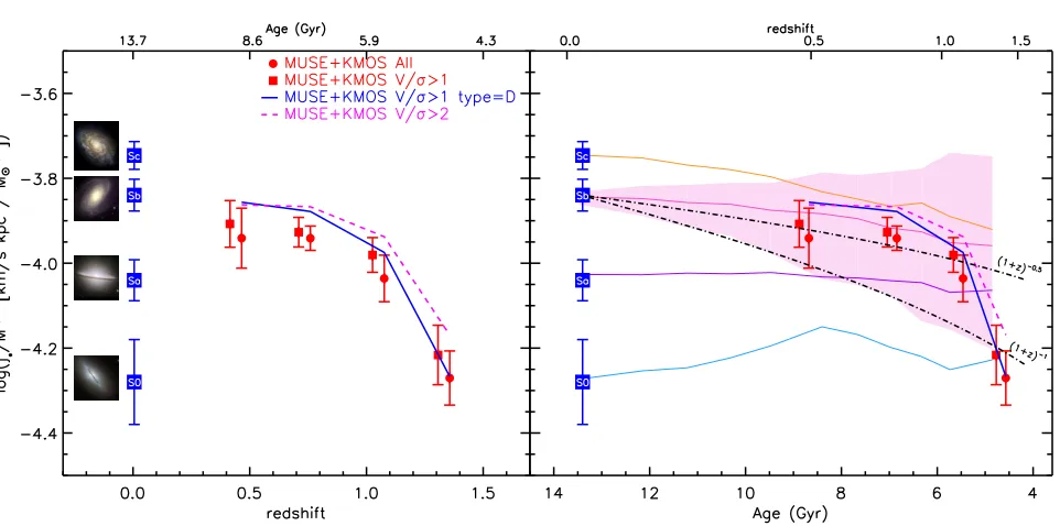
Lagos et al. (2016) show that the redshift evolution of the specific angular momentum of galaxies in theEAGLEsimulation depends sensitively on mass and star formation rate cuts applied. For example, in the model, massive galaxies which are classi-fied as “passive” around z ∼0.8 (those well below the “main-sequene”) show little / no evolution in specific angular momentum fromz ∼0.8 to z= 0, whilst “active” star-forming galaxies (i.e. on or above the “main-sequence”) can increase their specific angu-lar momentum1as rapidly asj⋆/ M⋆2/3 ∝(1 +z)3/2. In principle, these predictions can be tested by observations. .
1 We note that in the angular momentum comparisons below, quantitatively
similar results have been obtained from the Illustris simulation (Genel et al. 2015)
From the EAGLE model, the most direct method for cal-culating angular momentum galaxies is to sum the angular mo-mentum of each star particle that is associated with a galaxy (Jp=Pimiri×vi). However, this does not necessarily provide
a direct comparison with the observations data, where the angu-lar momentum is derived from the rotation curve and a measured galaxy sizes. To ensure a fair comparison between the observations and model can be made, we first calibrate the particle data in the
EAGLEgalaxies with their rotation curves. Schaller et al. (2015) ex-tract rotation curves forEAGLEgalaxies and show that over the ra-dial range where the galaxies are well resolved, their rotation curves are in good agreement with those expected for observed galax-ies of similar mass and bulge-to-disk ratio. We therefore select a subset of 5 000 galaxies atz ∼0 from theEAGLEsimulation that have stellar masses between M⋆= 108–1011.5M⊙and star forma-tion rates of SFR = 0.1–50 M⊙yr−1(i.e. reasonably well matched to the mass and star formation rate range of our observational sam-ple) and derive their rotation curves. In this calculation, we adopt the minimum of their gravitational potential as the galaxy center. We measure their stellar half mass radii (r1/2,⋆), and the circular velocity from the rotation curve at 3 Rdand then compute the
angu-lar momentum from the rotation curve (JRC= M⋆r1/2,⋆V(3 Rd)),
and compare this to the angular momentum derived from the par-ticle data (JP). The angular momentum of theEAGLEgalaxies2 measured from the particular data (JP) broadly agrees with that
es-timated from the rotation curves (JRC), although fitting the data
over the full range of J, we measure a sub-linear relation of log10(JRC) = (0.87±0.10) log10(JP) + 1.75±0.20. Although only
a small effect, this sub-linear offset occurs due to two factors. First, the sizes of the low-mass galaxies become comparable to the
∼1 kpc gravitational softening length of the simulation; and sec-ond, at lower stellar masses, the random motions of the stars have a larger contribution to the total dynamical support. Nevertheless, in all of the remaining sections (and to be consistent with the obser-vational data) we first calculate the “particle” angular momentum ofEAGLEgalaxies and then convert these to the “rotation-curve” angular momentum.
To test how well theEAGLEmodel reproduces the observed mass–specific angular momentum sequence atz= 0, in Fig. 8 we plot the specific angular momentum (j⋆=J/M⋆) of ∼50 late-type galaxies from the observational study of Romanowsky & Fall (2012) and also include the observations of 16 nearby spirals from the The HINearby Galaxy Survey (THINGS; Walter et al. 2008) as discussed in Obreschkow & Glazebrook (2014). As discussed in
§1, these local disks follow a correlation ofj⋆∝M2⋆/3with a scat-ter ofσlog j∼0.2 dex. We overlay the specific angular momentum
of galaxies atz= 0 from the theEAGLEsimulation, colour coded by their rest-frame(g−r)colour (Trayford et al. 2015). This high-lights that theEAGLEmodel provides a reasonable match to the
z= 0 scaling inj⋆∝M2⋆/3 in both normalisation and scatter. Fur-thermore, the colour-coding highlights that, at fixed stellar mass, the blue star-forming galaxies (late-types) have higher angular mo-mentum compared than those with redder (early-type) colours. A similar conclusion was reported by Zavala et al. (2016) who sep-arated galaxies inEAGLEin to early versus late types using their stellar orbits, identifying the same scaling between specific angular momentum and stellar mass for the late-types. Lagos et al. (2016)
2 We note that Lagos et al. (2016) show that inEAGLEthe value ofJ⋆and
the scaling betweenJ⋆and stellar mass is insensitive to whether an aperture
Figure 8. Left: Specific angular momentum (j⋆=J/ M⋆) of late- and early- type galaxies at z= 0 from Romanowsky & Fall (2012) and
Obreschkow & Glazebrook (2014) (R&F 2012 and O&G 2014 respectively), both of which follow a scaling ofj⋆ ∝M2⋆/3. We also show the specific
an-gular momentum of galaxies atz= 0 from theEAGLEsimulation (reference model) with the colour scale set by the rest-frameg−rcolours of the galaxies. The solid line shows the median (and dotted lines denote the 68% distribution width) of theEAGLEgalaxies. For comparison with otherEAGLEmodels, we also include the evolution ofj⋆–M⋆from the “constant feedback” FBconst model (dashed line). Right: The specific angular momentum for the high-redshift
galaxies in our MUSE and KMOS sample. We split the high-redshift sample in to those galaxies with the best sampled dynamics / rotation curves (which we denoteq= 1) and those with less well constrained rotation curves (q= 2). In the lower right corner we show the typical error bar, estimated using a combination of errors on the stellar mass, and uncertainties in the inclination and circular velocity measurement. We also include on the plot the unresolved galaxies from our sample using the limits on their sizes and velocity dispersions (the latter to provide an estimate of the upper limit onvc). The median specific angular momentum (and bootstrap error) in bins of log10(M⋆) = 0.3 dex is also shown. The grey-scale shows the predicted distribution atz ∼1 from theEAGLE simulation and we plot the median specific angular momentum in bins of stellar mass as well as theEAGLEz= 0 model from the left-hand panel. Although there is considerable scatter in the high-redshift galaxy sample, atz∼1, there are very few high stellar mass galaxies with specific angular momentum as large as comparably massive local spirals, suggesting that most of the accretion of high angular momentum material must occur belowz∼1.
also extend the analysis to investigate other morphological proxies such as spin, gas fraction, (u−r) colour, concentration and stellar age and in all cases, the results indicate that galaxies that have low specific angular momentum (at fixed stellar mass) are gas poor, red galaxies with higher stellar concentration and older mass-weighted ages.
In Fig. 8 we also show the predicted scaling between stellar mass and specific angular momentum fromEAGLEatz= 1 after ap-plying our mass and star formation rate limits to the galaxies in the model. This shows thatEAGLEpredicts the same scaling between specific angular momentum and stellar mass atz= 0 andz= 1 with
j⋆ ∝M2⋆/3, with a change in normalisation such that galaxies at
z∼1 (at fixed stellar mass) have systematically lower specific an-gular momentum by∼0.2 dex than those atz ∼0. We will return to this comparison in§4.
Before discussing the high-redshift data, we note that one of the goals of the EAGLEsimulation is to test sub-grid recipes for star-formation and feedback. The sub-grid recipes in the EAGLE
“reference model” are calibrated to match the stellar mass function atz= 0, but this model is not unique. For example, in the reference model the energy from star-formation is coupled to the ISM accord-ing to the local gas density and metallicity. This density dependence has the effect that outflows are able to preferentially expel material
from centers of galaxies, where the gas has low angular momentum. However, as discussed by Crain et al. (2015), in otherEAGLE mod-els that also match thez= 0 stellar mass function, the energetics of the outflows are coupled to the ISM in different ways, with im-plications for the angular momentum. For example, in the FBconst model, the energy from star formation is distributed evenly in to the surrounding ISM, irrespective of local density and metallicity. Since this model also matches thez= 0 stellar mass function, and so it is instructive to compare the angular momentum of the galax-ies in this model compared to the reference model. In Fig. 8 we also overlay thez= 0 relation between the specific angular momentum (j⋆) and stellar mass (M⋆) in theEAGLEFBconst model. For stellar
![Figure 2. Left: [OII] luminosity function for the star-forming galaxies in our sample from the 18 MUSE IFU pointings](https://thumb-us.123doks.com/thumbv2/123dok_us/9382959.441406/5.612.58.533.114.310/figure-left-luminosity-function-forming-galaxies-sample-pointings.webp)