warwick.ac.uk/lib-publications
Manuscript version: Author’s Accepted Manuscript
The version presented in WRAP is the author’s accepted manuscript and may differ from the
published version or Version of Record.
Persistent WRAP URL:
http://wrap.warwick.ac.uk/109823
How to cite:
Please refer to published version for the most recent bibliographic citation information.
If a published version is known of, the repository item page linked to above, will contain
details on accessing it.
Copyright and reuse:
The Warwick Research Archive Portal (WRAP) makes this work by researchers of the
University of Warwick available open access under the following conditions.
Copyright © and all moral rights to the version of the paper presented here belong to the
individual author(s) and/or other copyright owners. To the extent reasonable and
practicable the material made available in WRAP has been checked for eligibility before
being made available.
Copies of full items can be used for personal research or study, educational, or not-for-profit
purposes without prior permission or charge. Provided that the authors, title and full
bibliographic details are credited, a hyperlink and/or URL is given for the original metadata
page and the content is not changed in any way.
Publisher’s statement:
Please refer to the repository item page, publisher’s statement section, for further
information.
RANDOM ADVECTION-DIFFUSION EQUATIONS
ANA DJURDJEVAC, CHARLES M. ELLIOTT, RALF KORNHUBER, AND THOMAS RANNER
Abstract. In this paper, we introduce and analyse a surface finite element discretization of advection-diffusion equations with uncertain coefficients on evolving hypersurfaces. After stating unique solvability of the resulting semi-discrete problem, we prove optimal error bounds for the semi-semi-discrete solution and Monte-Carlo samplings of its expectation in appropriate Bochner spaces. Our theoretical findings are illustrated by numerical experiments in two and three space dimensions.
1. Introduction
Surface partial differential equations, i.e., partial differential equations on sta-tionary or evolving surfaces, have become a flourishing mathematical field with numerous applications, e.g., in image processing [26], computer graphics [6], cell biology [21,34], and porous media [32]. The numerical analysis of surface partial differential equations can be traced back to the pioneering paper of Dziuk [15] on the Laplace-Beltrami equation. Meanwhile there are various extensions to moving hypersurfaces such as, e.g., evolving surface finite element methods [16,17] or trace finite element methods [36], and an abstract framework for parabolic equations on evolving Hilbert spaces [1,2].
Though uncertain parameters are rather the rule than the exception in many applications and though partial differential equations with random coefficients have been intensively studied over the last years (cf., e.g., the monographs [31] and [29]), the numerical analysis of random surface partial differential equations still appears to be in its infancy.
In this paper, we present random evolving surface finite element methods for the advection-diffusion equation
∂•u− ∇Γ(α∇Γu) +u∇Γ·v =f
on an evolving compact hypersurface Γ(t) ⊂ Rn, n = 2, 3, with a uniformly bounded random coefficient α and deterministic velocity v on a compact time intervall t ∈ [0, T]. Here ∂• denotes the path-wise material derivative and ∇Γ
is the tangential gradient. While the analysis and numerical analysis of random advection-diffusion equations is well developed in the flat case [8, 25, 28, 33], to
2010Mathematics Subject Classification. 65N12, 65N30, 65C05.
Key words and phrases. geometric partial differential equations, surface finite elements, ran-dom advection-diffusion equation, uncertainty quantification.
The research of TR was funded by the Engineering and Physical Sciences Research Council (EPSRC EP/J004057/1). The research of CME was partially supported by the Royal Society via a Wolfson Research Merit Award and by the EPSRC programme grant (EP/K034154/1) EQUIP.
1
our knowledge, existence, uniqueness and regularity results for curved domains have been first derived only recently in [14]. Following Dziuk & Elliott [16], the space discretization is performed by random piecewise linear finite element func-tions on simplicial approximafunc-tions Γh(t) of the surface Γ(t),t∈[0, T]. We present
optimal error estimates for the resulting semi-discrete scheme which then provide corresponding error estimates for expectation values and Monte-Carlo approxima-tions. Application of efficient solution techniques, such as adaptivity [13], multigrid methods [27], and Multilevel Monte-Carlo techniques [3, 9, 10] is very promising but beyond the scope of this paper. In our numerical experiments we investigate a corresponding fully discrete scheme based on an implicit Euler method and observe optimal convergence rates.
The paper is organized as follows. We start by setting up some notation, the notion of hypersurfaces, function spaces, and material derivatives in order to de-rive a weak formulation of our problem according to [14]. Section 3 is devoted to the random ESFEM discretization in the spirit of [16] leading to the precise formulation and well-posedness of our semi discretization in space presented in Sec-tion4. Optimal error estimates for the approximate solution, its expectation and a Monte-Carlo approximation are contained in Section 5. The paper concludes with numerical experiments in two and three space dimensions suggesting that our optimal error estimates extend to corresponding fully discrete schemes.
2. Random advection-diffusion equations on evolving hypersurfaces
Let (Ω,F,P) be a complete probability space with sample space Ω, a σ-algebra of eventsFand a probabilityP:F →[0,1]. In addition, we assume thatL2(Ω) is a separable space. For this assumption it suffices to assume that (Ω,F,P) is separable [23, Exercise 43.(1)]. We consider a fixed finite time interval [0, T], where T ∈
(0,∞).Furthermore, we denote byD((0, T);V) the space of infinitely differentiable functions with values in a a Hilbert spaceV and compact support in (0, T).
2.1. Hypersurfaces. We first recall some basic notions and results concerning hypersurfaces and Sobolev spaces on hypersurfaces. We refer to [11] and [19] for more details.
Let Γ⊂Rn+1 (n= 1,2) be aC3-compact, connected, orientable,n-dimensional hypersurface without boundary. For a function f: Γ→R allowing for a differen-tiable extension ˜f to an open neighbourhood of Γ inRn+1 we define thetangential
gradient by
(2.1) ∇Γf(x) :=∇f˜(x)− ∇f˜(x)·ν(x)ν(x), x∈Γ,
whereν(x) denotes the unit normal to Γ.
Note that ∇Γf(x) is the orthogonal projection of ∇f˜onto the tangent space
to Γ at x (thus a tangential vector). It depends only on the values of ˜f on Γ [19, Lemma 2.4], which makes the definition (2.1) independent of the extension ˜f. The tangential gradient is a vector-valued quantity and for its components we use the notation∇Γf(x) = (D1f(x), . . . , Dn+1f(x)).TheLaplace-Beltrami operator is
defined by
∆Γf(x) =∇Γ· ∇Γf(x) =
n+1 X
i=1
In order to prepare weak formulations of PDEs on Γ, we now introduce Sobolev spaces on surfaces. To this end, letL2(Γ) denote the Hilbert space of all measurable functions f: Γ→R such thatkfkL2(Γ):=
R Γ|f(x)|
21/2 is finite. We say that a
functionf ∈L2(Γ) has a weak partial derivativegi=Dif ∈L2(Γ),(i={1, . . . , n+
1}), if for every functionφ∈ C1(Γ) and everyithere holds Z
Γ
f Diφ=−
Z
Γ φgi+
Z
Γ f φHνi
whereH =−∇Γ·ν denotes the mean curvature. The Sobolev spaceH1(Γ) is then
defined by
H1(Γ) ={f ∈L2(Γ)|Dif ∈L2(Γ), i= 1, . . . , n+ 1}
with the normkfkH1(Γ)= (kfk2L2(Γ)+k∇Γfk2L2(Γ))1/2.
For a description of evolving hypersurfaces we consider two approaches, starting with evolutions according to a given velocity field v. Here, we assume that Γ(t) satisfies the same properties as Γ(0) = Γ for everyt∈[0, T], and we set Γ0:= Γ(0).
Furthermore, we assume the existence of a flow, i.e., of a diffeomorphism
Φ0t(·) := Φ(·, t) : Γ0→Γ(t), Φ∈ C1([0, T],C1(Γ0)n+1)∩ C0([0, T],C3(Γ0)n+1),
that satisfies
(2.2) d
dtΦ 0
t(·) = v(t,Φ
0
t(·)), Φ
0
0(·) = Id(·),
with aC2-velocity field v : [0, T]×
Rn+1→Rn+1with uniformly bounded divergence (2.3) |∇Γ(t)·v(t)| ≤C ∀t∈[0, T].
It is sometimes convenient to alternatively represent Γ(t) as the zero level set of a suitable function defined on a subset of the ambient spaceRn+1. More precisely, under the given regularity assumptions for Γ(t), it follows by the Jordan-Brouwer theorem that Γ(t) is the boundary of an open bounded domain. Thus, Γ(t) can be represented as the zero level set
Γ(t) ={x∈ N(t)|d(x, t) = 0}, t∈[0, T],
of a signed distance function d=d(x, t) defined on an open neighborhoodN(t) of Γ(t) such that|∇d| 6= 0 fort∈[0, T]. Note thatd, dt,dxi,dxixj ∈ C
1(NT) withi, j= 1, . . . , n+ 1 holds for
NT := [
t∈[0,T]
N(t)× {t}.
We also choose N(t) such that for every x ∈ N(t) and t ∈ [0, T] there exists a uniquep(x, t)∈Γ(t) such that
(2.4) x=p(x, t) +d(x, t)ν(p(x, t), t),
and fix the orientation of Γ(t) by choosing the normal vector fieldν(x, t) :=∇d(x, t). Note that the constant extension of a functionη(·, t) : Γ(t)→RtoN(t) in normal direction is given byη−l(x, t) =η(p(x, t), t),p∈ N(t). Later on, we will use (2.4)
2.2. Function spaces. In this section, we define Bochner-type function spaces of random functions that are defined on evolving spaces. The definition of these spaces is taken from [14] and uses the idea from Alphonse et al. [1] to map each domain at timetto the fixed initial domain Γ0by a pull-back operator using the flow Φ0t. Note
that this approach is similar to Arbitrary Lagrangian Eulerian (ALE) framework. For eacht∈[0, T], let us define
V(t) :=L2(Ω, H1(Γ(t)))∼=L2(Ω)⊗H1(Γ(t)) (2.5)
H(t) :=L2(Ω, L2(Γ(t)))∼=L2(Ω)⊗L2(Γ(t)) (2.6)
where the isomorphisms hold because all considered spaces are separable Hilbert spaces (see [35]). The dual space of V(t) is the space V∗(t) =L2(Ω, H−1(Γ(t))),
whereH−1(Γ(t)) is the dual space ofH1(Γ(t)). Using the tensor product structure
of these spaces [22, Lemma 4.34], it follows thatV(t)⊂H(t)⊂V∗(t) is a Gelfand triple for every t ∈ [0, T]. For convenience we will often (but not always) write
u(ω, x) instead of u(ω)(x), which is justified by the tensor structure of the spaces. For an evolving family of Hilbert spacesX = (X(t))t∈[0,T], such as, e.g., V =
(V(t))t∈[0,T]orH = (H(t))t∈[0,T]we connect the spaceX(t) for fixedt∈[0, T] with
the initial spaceX(0) by using a family of so-called pushforward mapsφt:X(0)→
X(t), satisfying certain compatibility conditions stated in [1, Definition 2.4]. More precisely, we use its inverse mapφ−t:X(t)→X(0), called pullback map, to define
general Bochner-type spaces of functions defined on evolving spaces as follows (see [1,14])
L2X :=
u: [0, T]3t7→(¯u(t), t)∈ [
t∈[0,T]
X(t)× {t} |φ−(·)u¯(·)∈L2(0, T;X(0))
,
L2X∗:=
f : [0, T]3t7→( ¯f(t), t)∈ [
t∈[0,T]
X∗(t)× {t} |φ−(·)f¯(·)∈L2(0, T;X(0)∗)
.
In the following we will identifyu(t) = (u(t);t) withu(t). From [1, Lemma 2.15] it follows thatL2
X∗ and (L2X)∗ are isometrically
isomor-phic. The spacesL2
X andL
2
X∗ are separable Hilbert spaces [1, Corollary 2.11] with
the inner product defined as
(u, v)L2
X =
Z T
0
(u(t), v(t))X(t)dt (f, g)L2
X∗ =
Z T
0
(f(t), g(t))X∗(t)dt.
For the evolving familyH defined in (2.6) we define the pullback operatorφ−t:
H(t)→H(0) for fixedt∈[0, T] and eachu∈H(t) by
(φ−tu)(ω, x) :=u(ω,Φt0(x)), x∈Γ0= Γ(0), ω∈Ω,
utilizing the parametrisation Φ0
t of Γ(t) over Γ0. Exploiting V(t) ⊂ H(t), the
pullback operator φ−t:V(t)→V(0) is defined by restriction. It follows from [14,
Lemma 3.5] that the resulting spacesL2
V,L2V∗ andL2H are well-defined and
L2V ⊂L2H ⊂L2V∗
2.3. Material derivative. Following [14], we introduce a material derivative of sufficiently smooth random functions that takes spatial movement into account.
First let us define the spaces of pushed-forward continuously differentiable func-tions
CXj :={u∈L2X |φ−(·)u(·)∈ Cj([0, T], X(0))} forj ∈ {0,1,2}.
Foru∈ C1
V the material derivative∂•u∈ CV0 is defined by
(2.7) ∂•u:=φt
d
dtφ−tu
=ut+∇u·v.
More precisely, the material derivative of uis defined via a smooth extension ˜uof
utoNT with well-defined derivatives ∇u˜ and ˜ut and subsequent restriction to
GT :=[
t
Γ(t)× {t} ⊂ NT.
Since, due to the smoothness of Γ(t) and Φt0, this definition is independent of the
choice of particular extension ˜u, we simply writeuin (2.7).
Remark 2.1. Replacing classical derivatives in time by weak derivatives leads to a
weak material derivative∂•u∈L2V∗. It coincides with the strong material derivative
for sufficiently smooth functions. As we will concentrate on the smooth case later
on, we omit a precise definition here and refer to [14, Definition 3.9] for details.
2.4. Weak formulation and well-posedness. We consider an initial value prob-lem for an advection-diffusion equation on the evolving surface Γ(t),t∈[0, T], which in strong form reads
(2.8) ∂
•u− ∇
Γ·(α∇Γu) +u∇Γ·v =f u(0) =u0
.
Here the diffusion coefficient α and the initial functionu0 are random functions,
and we setf ≡0 for ease of presentation.
We will consider weak solutions of (2.8) from the space
(2.9) W(V, H) :={u∈LV2 |∂•u∈L2H}
where∂•ustands for the weak material derivative. W(V, H) is a separable Hilbert space with the inner product defined by
(u, v)W(V,H)= Z T
0 Z
Ω
(u, v)H1(Γ(t))+ Z T
0 Z
Ω
(∂•u, ∂•v)L2(Γ(t)).
Now aa weak solution of (2.8) is a solution of the following problem.
Problem 2.1(Weak form of the random advection-diffusion equation on{Γ(t)}).
Find u∈W(V, H)that point-wise satisfies the initial condition u(0) =u0 ∈V(0)
and
(2.10)
Z
Ω Z
Γ(t)
∂•u(t)ϕ+
Z
Ω Z
Γ(t)
α(t)∇Γu(t)· ∇Γϕ+ Z
Ω Z
Γ(t)
u(t)ϕ∇Γ·v(t) = 0,
for everyϕ∈L2(Ω, H1(Γ(t))) and a.e. t∈[0, T].
Existence and uniqueness can be stated on the following assumption.
Assumption 2.1. The diffusion coefficientαsatisfies the following conditions
b) α(ω,·,·) ∈ C1(GT) holds for
P-a.e ω ∈ Ω, which implies boundedness of
|∂•α(ω)|on GT, and we assume that this bound is uniform inω∈Ω.
c) αis uniformly bounded from above and below in the sense that there exist
positive constants αmin andαmax such that
(2.11) 0< αmin≤α(ω, x, t)≤αmax<∞ ∀(x, t)∈ GT
holds forP-a.e. ω∈Ω
and the initial function satisfies u0∈L2(Ω, H1(Γ0)).
The following proposition is a consequence of [14, Theorem 4.9].
Proposition 2.1. Let Assumption 2.1 hold. Then, under the given assumptions
on{Γ(t)}, there is a unique solutionu∈W(V, H)of Problem2.1and we have the
a priori bound
kukW(V,H)≤Cku0kV(0)
with some C∈R.
The following assumption of the diffusion coefficient will ensure regularity of the solution.
Assumption 2.2. Assume that there exists a constant C independent of ω ∈ Ω
such that
|∇Γα(ω, x, t)| ≤C ∀(x, t)∈ GT
holds forP-almost all ω∈Ω.
Note that (2.11) and Assumption 2.2 imply that kα(ω, t)kC1(Γ(t)) is uniformly
bounded in ω ∈ Ω. This will be used later to prove an H2(Γ(t)) bound. In the subsequent error analysis, we will assume further that u has a path-wise strong material derivative, i.e. thatu(ω)∈C1
V holds for allω∈Ω.
In order to derive a more convenient formulation of Problem 2.1with identical solution and test space, we introduce the time dependent bilinear forms
(2.12)
m(u, ϕ) :=
Z
Ω Z
Γ(t)
uϕ, g(v;u, ϕ) :=
Z
Ω Z
Γ(t)
uϕ∇Γ·v,
a(u, ϕ) :=
Z
Ω Z
Γ(t)
α∇Γu· ∇Γϕ, b(v;u, ϕ) := Z
Ω Z
Γ(t)
B(ω,v)∇Γu· ∇Γϕ
for u, ϕ∈ L2(Ω, H1(Γ(t))) and each t ∈[0, T]. The tensor B in the definition of b(v;u, ϕ) takes the form
B(ω,v) = (∂•α+α∇Γ·v)Id−2αDΓ(v)
with Id denoting the identity in (n+ 1)×(n+ 1) and (DΓv)ij =Djvi. Note that
(2.3) and the uniform boundedness of ∂•α onGT imply that |B(ω,v)| ≤C holds
P-a.e. ω∈Ω with some C∈R.
The transport formula for the differentiation of the time dependent surface in-tegral then reads (see e.g. [14])
d
dtm(u, ϕ) =m(∂
•u, ϕ) +m(u, ∂•ϕ) +g(v;u, ϕ),
(2.13)
Problem 2.2(Weak form of the random advection-diffusion equation on{Γ(t)}).
Find u∈W(V, H)that point-wise satisfies the initial condition u(0) =u0 ∈V(0)
and
(2.14) d
dtm(u, ϕ) +a(u, ϕ) =m(u, ∂
•ϕ) ∀ϕ∈W(V, H).
This formulation will be used in the sequel.
3. Evolving simplicial surfaces
As a first step towards a discretization of the weak formulation (2.14) we now consider simplicial approximations of the evolving surface Γ(t),t∈[0, T]. Let Γh,0
be an approximation of Γ0consisting of nondegenerate simplices{Ej,0}Nj=1=:Th,0
with vertices {Xj,0}Jj=1 ⊂Γ0 such that the intersection of two different simplices
is a common lower dimensional simplex or empty. For t ∈ [0, T], we let the ver-tices Xj(0) = Xj,0 evolve with the smooth surface velocity Xj0(t) = v(Xj(t), t),
j= 1, . . . , J, and consider the approximation Γh(t) of Γ(t) consisting of the
corre-sponding simplices{Ej(t)}Mj=1=:Th(t). We assume that shape regularity ofTh(t)
holds uniformly int∈[0, T] and thatTh(t) is quasi-uniform, uniformly in time, in the sense that
h:= sup
t∈(0,T)
max
E(t)∈Th(t)
diamE(t)≥ inf
t∈(0,T)
min
E(t)∈Th(t)
diamE(t)≥ch
holds with some c ∈ R. We also assume that Γh(t) ⊂ N(t) for t ∈[0, T] and, in
addition to (2.4), that for everyp∈Γ(t) there is a uniquex(p, t)∈Γh(t) such that
(3.1) p=x(p, t) +d(x(p, t), t)ν(p, t).
Note that Γh(t) can be considered as interpolation of Γ(t) in {Xj(t)}Jj=1 and a
discrete analogue of the space time domainGT is given by
Gh T :=
[
t
Γh(t)× {t}.
We define the tangential gradient of a sufficiently smooth functionηh: Γh(t)→R in an element-wise sense, i.e., we set
∇Γhηh|E =∇ηh− ∇ηh·νhνh, E∈ Th(t).
Hereνhstands for the element-wise outward unit normal toE ⊂Γh(t). We use the
notation∇Γhηh= (Dh,1ηh, . . . , Dh,n+1ηh).
We define the discrete velocityVhof Γh(t) by interpolation of the given velocity v,
i.e. we set
Vh(X(t), t) := ˜Ihv(X(t), t), X(t)∈Γh(t),
with ˜Ihdenoting piecewise linear interpolation in{Xj(t)}Jj=1.
We consider the Gelfand triple on Γh(t)
(3.2) L2(Ω, H1(Γh(t)))⊂L2(Ω, L2(Γh(t)))⊂L2(Ω, H−1(Γh(t)))
and denote
Vh(t) :=L2(Ω, H1(Γh(t))) and Hh(t) :=L2(Ω, L2(Γh(t))).
As in the continuous case, this leads to the following Gelfand triple of evolving Bochner-Sobolev spaces
(3.3) L2V
h(t)⊂L
2
Hh(t)⊂L
2 V∗
The discrete velocityVh induces a discrete strong material derivative in terms
of an element-wise version of (2.7), i.e., for sufficiently smooth functionsφh∈L2Vh
and anyE(t)∈Γh(t) we set
(3.4) ∂h•φh|E(t):= (φh,t+Vh· ∇φh)|E(t).
We define discrete analogues to the bilinear forms introduced in (2.12) onVh(t)× Vh(t) according to
mh(uh, ϕh) :=
Z
Ω Z
Γh(t)
uhϕh, gh(Vh;uh, ϕh) :=
Z
Ω Z
Γh(t)
uhϕh∇Γh·Vh,
ah(uh, ϕh) :=
Z
Ω Z
Γh(t)
α−l∇Γhuh· ∇Γhϕh,
bh(Vh;φ, Uh) :=
X
E(t)∈Th(t)
Z
Ω Z
E(t)
Bh(ω, Vh)∇Γhφ· ∇ΓhUh
involving the tensor
Bh(ω, Vh) = (∂h•α
−l+α−l∇
Γh·Vh)Id−2α
−lD h(Vh)
denoting (Dh(Vh))ij =Dh,jVhi. Here, we denote
(3.5) α−l(ω, x, t) :=α(ω, p(x, t), t) ω∈Ω, (x, t)∈ Gh T
exploiting{Γh(t)} ⊂ N(t) and (2.4). Laterα−l will be called the inverse lift ofα.
Note thatα−lsatisfies a discrete version of Assumption2.1and2.2. In particular,
α−l is an F ⊗ B(Gh
T)-measurable function, α−l(ω,·,·)|ET ∈ C
1(E
T) for all
space-time elements ET :=StE(t)× {t}, andαmin≤α−l(ω, x, t)≤αmax for allω∈Ω,
(x, t)∈ Gh T.
The next lemma provides a uniform bound for the divergence ofVhand the norm
of the tensorBh that follows from the geometric properites of Γh(t) in analogy to
[20, Lemma 3.3].
Lemma 3.1. Under the above assumptions on{Γh(t)}, it holds
sup
t∈[0,T]
k∇Γh·VhkL∞(Γh(t))+kBhkL2(Ω,L∞(Γh(t)))
≤c sup
t∈[0,T]
kv(t)kC2(NT)
with a constant c depending only on the initial hypersurface Γ0 and the uniform
shape regularity and quasi-uniformity ofTh(t).
Since the probability space does not depend on time, the discrete analogue of the corresponding transport formulae hold, where the discrete material velocity and discrete tangential gradients are understood in an element-wise sense. The resulting discrete result is stated for example in [17, Lemma 4.2]. The following lemma follows by integration over Ω.
Lemma 3.2 (Transport lemma for triangulated surfaces). Let {Γh(t)} be a
fam-ily of triangulated surfaces evolving with discrete velocity Vh. Let φh, ηh be time
dependent functions such that the following quantities exist. Then
d dt
Z
Ω Z
Γh(t)
φh=
Z
Ω Z
Γh(t)
∂•hφh+φh∇Γh·Vh.
In particular,
(3.6) d
dtmh(φh, ηh) =m(∂ •
4. Evolving surface finite element methods
Following [16], we now introduce an evolving surface finite element discretization (ESFEM) of Problem2.2.
4.1. Finite elements on simplicial surfaces. For eacht ∈[0, T] we define the
evolving finite element space
(4.1) Sh(t) :={η∈ C(Γh(t))|ηE is affine∀E∈ Th(t)}.
We denote by {χj(t)}j=1,...,J the nodal basis of Sh(t), i.e. χj(Xi(t), t) = δij
(Kronecker-δ). These basis functions satisfy the transport property [17, Lemma 4.1]
(4.2) ∂h•χj= 0.
We consider the following Gelfand triple
(4.3) Sh(t)⊂Lh(t)⊂Sh∗(t),
where all three spaces algebraically coincide but are equipped with different norms inherited from the corresponding continuous counterparts, i.e.,
Sh(t) := (Sh(t),k · kH1(Γh(t))) and Lh(t) := (Sh(t),k · kL2(Γh(t))).
The dual spaceS∗h(t) consists of all continuous linear functionals onSh(t) and is
equipped with the standard dual norm
kψkS∗
h(t):= sup
{η∈Sh(t)| kηkH1 (Γh(t))=1}
|ψ(η)|.
Note that all three norms are equivalent as norms on finite dimensional spaces, which implies that (4.3) is the Gelfand triple. As a discrete counterpart of (3.2), we introduce the Gelfand triple
(4.4) L2(Ω, Sh(t))⊂L2(Ω, Lh(t))⊂L2(Ω, S∗h(t)).
Setting
Vh(t) :=L2(Ω, Sh(t)) Hh(t) :=L2(Ω, Lh(t)) Vh∗(t) :=L
2(Ω, S∗
h(t))
we obtain the finite element analogue
(4.5) L2V
h(t)⊂L
2
Hh(t)⊂L
2
V∗
h(t)
of the Gelfand triple (3.3) of evolving Bochner-Sobolev spaces. Let us note that since the sample space Ω is independent of time, it holds
(4.6) L2(Ω, L2X)∼=L2(Ω)⊗L2X ∼=L2L2(Ω,X)
for any evolving family of separable Hilbert spaces X (see, e.g., Section 3). We will exploit this isomorphism forX =Sh in the following definition of the solution
space for the semi-discrete problem, where we will rather consider the problem in a path-wise sense.
We define the solution space for the semi-discrete problem as the space of func-tions that are smooth for each path in the sense that φh(ω) ∈ CS1h holds for all
ω∈Ω. Hence,∂•hφh is defined path-wise for path-wise smooth functions. In
addi-tion, we require∂h•φh(t)∈Hh(t) to define the semi-discrete solution space
The scalar product of this space is defined by
(Uh, φh)Wh(Vh,Hh):=
Z T
0 Z
Ω
(Uh, φh)H1(Γ
h(t))+
Z T
0 Z
Ω
(∂•hUh, ∂h•φh)L2(Γ
h(t))
with the associated normk · kWh(Vh,Hh).
The semi-discrete approximation of Problem2.2, on{Γh(t)}now reads as follows.
Problem 4.1(ESFEM discretization in space). FindUh∈Wh(Vh, Hh)that
point-wise satisfies the initial conditionUh(0) =Uh,0 ∈Vh(0)and
(4.7) d
dtmh(Uh, ϕ) +ah(Uh, ϕ) =mh(Uh, ∂ •
hϕ) ∀ϕ∈Wh(Vh, Hh).
In contrast to W(V, H), the semidiscrete space Wh(Vh, Hh) is not complete so
that the proof of the following existence and stability result requires a different kind of argument.
Theorem 4.1. The semi-discrete problem (4.9) has a unique solutionUh∈Wh(Vh, Hh)
which satisfies the stability property
(4.8) kUhkW(Vh,Hh)≤CkUh,0kVh(0)
with a mesh-independent constantCdepending only onT,αmin, and the bound for
k∇Γh·Vhk∞ from Lemma3.1.
Proof. In analogy to Subsection2.4, Problem4.1is equivalent to findUh∈Wh(Vh, Hh)
that point-wise satisfies the initial conditionUh(0) =Uh,0 ∈Vh(0) and
(4.9) mh(∂h•Uh, ϕ) +a(Uh, ϕ) +g(Vh;Uh, ϕ) = 0
for everyϕ∈L2(Ω, S
h(t)) and a.e. t∈[0, T].
Letω ∈Ω be arbitrary but fixed. We start with considering the deterministic path-wise problem to findUh(ω)∈ CS1h such thatUh(ω; 0) =Uh,0(ω) and
(4.10)
Z
Γh(t)
∂h•Uh(ω)ϕ+
Z
Γh(t)
α−l(ω)∇ΓhUh(ω)· ∇Γhϕ+
Z
Γh(t)
Uh(ω)ϕ∇Γh·Vh= 0
holds for all ϕ∈Sh(t) and a.e. t ∈[0, T]. Following Dziuk & Elliott [17, Section
4.6], we insert the nodal basis representation
(4.11) Uh(ω, t, x) =
J
X
j=1
Uj(ω, t)χj(x, t)
into (4.10) and take ϕ = χi(t) ∈ Sh(t), i = 1, . . . , J, as test functions. Now the
transport property (4.2) implies
J
X
j=1 ∂ ∂tUj(ω)
Z
Γh(t)
χjχi + J
X
j=1 Uj(ω)
Z
Γh(t)
α−l(ω)∇Γhχj· ∇Γhχi
(4.12)
+
J
X
j=1 Uj(ω)
Z
Γh(t)
χjχi∇Γh·Vh= 0.
We introduce the evolving mass matrixM(t) with coefficients
M(t)ij :=
Z
Γh(t)
and the evolving stiffness matrixS(ω, t) with coefficients
S(ω, t)ij :=
Z
Γh(t)
α−l(ω, t)∇Γhχj(t)∇Γhχi(t).
From [17, Proposition 5.2] it follows
dM dt =M
0
where
M0(t)ij :=
Z
Γh(t)
χj(t)χi(t)∇Γh·Vh(t).
Therefore, we can write (4.12) as the following linear initial value problem
(4.13) ∂
∂t(M(t)U(ω, t)) +S(ω, t)U(ω, t) = 0, U(ω,0) =U0(ω),
for the unknown vector U(ω, t) = (Uj(ω, t))Ji=1 of coefficient functions. As in [17],
there exists an unique path-wise semi-discrete solution Uh(ω) ∈ CS1h, since the
matrixM(t) is uniformly positive definite on [0, T] and the stiffness matrixS(ω, t) is positive semi-definite for everyω ∈Ω. Note that the time regularity of Uh(ω)
follows fromM,S(ω)∈C1(0, T) which in turn is a consequence of our assumptions on the time regularity of the evolution of Γh(t).
The next step is to prove the measurability of the map Ω3ω 7→Uh(ω)∈ CS1h.
OnC1
Sh we consider the Borelσ−algebra induced by the norm
(4.14) kUhk2 C1
Sh
:=
Z T
0
kUh(t)k2H1(Γ
h(t))+k∂
•
hUh(t)k2L2(Γ
h(t)).
We write (4.12) in the following form
∂
∂tU(ω, t) +A(ω, t)U(ω, t) = 0, U(ω,0) =U0(ω),
where
A(ω, t) :=M−1(t) (M0(t) +S(ω, t)).
As Uh,0 ∈ Vh(0), the function ω 7→ U0(ω) is measurable and since α−l is a
F ⊗ B(Gh
T)-measurable function, it follows from Fubini’s Theorem [23, Sec. 36,
Thm. C] that
Ω3ω7→(U0(ω), A(ω))∈RJ× C1 [0, T],RJ,k · k∞
is measurable function. Utilizing Gronwall’s lemma it can be shown that the map-ping
RJ× C1 [0, T],RJ,k · k∞3(U0, A)7→U ∈ C1 [0, T],RJ,k · k∞
is continuous. Furthermore, the mapping
C1 [0, T],RJ,k · k∞3U 7→U ∈ C1 [0, T],RJ,k · k2
with
kUk2 2:=
Z T
0
kU(t)k2
RJ+k
d dtU(t)k
2
RJ
is continuous. Exploiting that the triangulation Th(t) of Γh(t) is quasi-uniform,
uniformly in time, the continuity of the linear mapping
C1 [0, T],RJ ,k · k2
follows from the triangle inequality and the Cauchy-Schwarz inequality. We finally conclude that the function
Ω3ω7→Uh(ω)∈ CS1h
is measurable as a composition of measurable and continuous mappings.
The next step is to prove the stability property (4.8). For each fixed ω ∈ Ω, path-wise stability results from [17, Lemma 4.3] imply
(4.15) kUh(ω)k2C1
Sh
≤CkUh,0(ω)k2H1(Γh(0))
where C = C(αmin, αmax, Vh, T,GhT) is independent of ω and Uh,0(x) ∈ L2(Ω).
Integrating (4.15) over Ω we get the bound
kUhkW(Vh,Hh)=kUhk
2
L2(Ω,C1
Sh)
≤CkUh,0k2Vh(0).
In particular, we haveUh∈Wh(Vh, Hh).
It is left to show that Uh solves (4.9) and thus Problem 4.1. Exploiting the
tensor product structure of the test spaceL2(Ω, S
h(t))∼=L2(Ω)⊗Sh(t) (see (4.6)),
we find that
{ϕh(x, t)η(ω)|ϕh(t)∈Sh(t), η∈L2(Ω)} ⊂L2(Ω)⊗Sh(t)
is a dense subset of L2(Ω, S
h(t)). Taking any test functionϕh(x, t)η(ω) from this
dense subset, we first insertϕh(x, t)∈Sh(t) into the pathwise problem (4.10), then
multiply withη(ω), and finally integrate over Ω to establish (4.9). This completes
the proof.
4.2. Lifted finite elements. We exploit (3.1) to define the lift ηl
h(·, t) : Γ(t)→R
of functionsηh(·, t) : Γh(t)→Rby
ηhl(p, t) :=ηh(x(p, t)), p∈Γ(t).
Conversely, (2.4) is utilized to define the inverse liftη−l(·, t) : Γh(t)→Rof functions
η(·, t) : Γ(t)→Rby
η−l(x, t) :=η(p(x, t), t), x∈Γh(t).
These operators are inverse to each other, i.e., (η−l)l = (ηl)−l = η, and, taking
characteristic functions ηh, each element E(t) ∈ Th(t) has its unique associated
lifted elemente(t)∈ Tl
h(t). Recall that the inverse liftα−1of the diffusion coefficient
αwas already introduced in (3.5).
The next lemma states equivalence relations between corresponding norms on Γ(t) and Γh(t) that follow directly from their deterministic counterparts (see [15]).
Lemma 4.1. Let t ∈ [0, T], ω ∈ Ω, and let ηh(ω) : Γh(t) → R with the lift
ηhl(ω) : Γ → R. Then for each plane simplex E ⊂ Γh(t) and its curvilinear lift
e⊂Γ(t), there is a constant c >0 independent of E, h, t, andω such that
1
c kηhkL2(Ω,L2(E))≤ kη
l
hkL2(Ω,L2(e))≤ckηhkL2(Ω,L2(E))
(4.16)
1
c k∇ΓhηhkL2(Ω,L2(E))≤ k∇Γη
l
hkL2(Ω,L2(e))≤ck∇ΓhηhkL2(Ω,L2(E))
(4.17)
1
c k∇ 2
ΓhηhkL2(Ω,L2(E))≤ck∇
2 Γη
l
hkL2(Ω,L2(e))+chk∇ΓηhlkL2(Ω,L2(e)),
(4.18)
The motion of the vertices of the triangles E(t) ∈ {Th(t)} induces a discrete velocity vh of the surface {Γ(t)}. More precisely, for a given trajectory X(t) of
a point on {Γh(t)} with velocityVh(X(t), t) the associated discrete velocity vh in
Y(t) =p(X(t), t) on Γ(t) is defined by
(4.19) vh(Y(t), t) =Y0(t) =
∂p
∂t(X(t), t) +Vh(X(t), t)· ∇p(X(t), t).
The discrete velocity vh gives rise to a discrete material derivative of functions
ϕ∈L2V in an element-wise sense, i.e., we set
∂h•ϕ|e(t):= (ϕt+ vh· ∇ϕ)|e(t)
for alle(t)∈ Tl
h(t), whereϕtand∇ϕare defined via a smooth extension, analogous
to the definition (2.7).
We introduce a lifted finite element space by
Shl(t) :={ηl∈ C(Γ(t))|η∈Sh(t)}.
Note that there is a unique correspondence between each element η ∈ Sh(t) and
ηl∈Sl
h(t). Furthermore, one can show that for everyφh∈Sh(t) here holds
(4.20) ∂•h(φlh) = (∂h•φh)l.
Therefore, by (4.2) we get
∂h•χlj= 0.
We finally state an analogon to the transport Lemma3.2on simplicial surfaces.
Lemma 4.2. (Transport lemma for smooth triangulated surfaces.)
Let Γ(t)be an evolving surface decomposed into curved elements {Th(t)} whose
edges move with velocityvh. Then the following relations hold for functionsϕh, uh
such that the following quantities exist
d dt
Z
Ω Z
Γ(t) ϕh=
Z
Ω Z
Γ(t)
∂h•ϕh+ϕh∇Γ·vh.
and
(4.21) d
dtm(ϕ, uh) =m(∂ •
hϕh, uh) +m(ϕh, ∂h•uh) +g(vh;ϕh, uh).
Remark 4.1. Let Uh be the solution of the semi-discrete Problem 4.1 with initial
conditionUh(0) =Uh,0 and letuh=Uhl withuh(0) =uh,0=Uh,l0 be its lift. Then,
as a consequence of Theorem 4.1,(4.20), and Lemma4.1, the following estimate
(4.22) kuhkW(V,H)≤C0kuh(0)kV(0)
holds with C0 depending on the constants C andc appearing in Theorem4.1 and
Lemma4.1, respectively.
5. Error estimates
Furthermore, we need to show that the extended definitions of the interpolation operator and Ritz projection operator are integrable with respect toP.
We start with an interpolation error estimate for functionsη∈L2(Ω, H2(Γ(t))), where the interpolation Ihη is defined as the lift of piecewise linear nodal
inter-polation Iehη ∈ L2(Ω, Sh(t)). Note that Ieh is well-defined, because the vertices
(Xj(t))Jj=1 of Γh(t) lie on the smooth surface Γ(t) andn= 2, 3.
Lemma 5.1. The interpolation error estimate
kη−IhηkH(t)+hk∇Γ(η−Ihη)kH(t)
≤ch2 k∇2
ΓηkH(t)+hk∇ΓηkH(t)
(5.1)
holds for all η ∈ L2(Ω, H2(Γ(t))) with a constant c depending only on the shape
regularity ofΓh(t).
Proof. The proof of the lemma follows directly from the deterministic case and
Lemma4.1.
We continue with estimating the geometric perturbation errors in the bilinear forms.
Lemma 5.2. Let t ∈ [0, T] be fixed. For Wh(·, t) and φh(·, t) ∈ L2(Ω, Sh(t))
with corresponding lifts wh(·, t) and ϕh(·, t) ∈ L2(Ω, Slh(t)) we have the following
estimates of the geometric error
|m(wh, ϕh)−mh(Wh, φh)| ≤ch2kwhkH(t)kϕhkH(t)
(5.2)
|a(wh, ϕh)−ah(Wh, φh)| ≤ch2k∇ΓwhkH(t)k∇ΓϕhkH(t)
(5.3)
|g(vh;wh, ϕh)−gh(Vh;Wh, φh)| ≤ch2kwhkV(t)kϕhkV(t)
(5.4)
|m(∂h•wh, ϕh)−mh(∂h•Wh, φh)| ≤ch2k∂h•whkH(t)kϕkH(t).
(5.5)
Proof. The assertion follows from uniform bounds of α(ω, t) and ∂h•α(ω, t) with
respect toω∈Ω together with corresponding deterministic results obtained in [17]
and [30].
Since the velocity v of Γ(t) is deterministic, we can use [17, Lemma 5.6] to control its deviation from the discrete velocity vh on Γ(t). Furthermore, [17, Corollary
5.7] provides the following error estimates for the continuous and discrete material derivative.
Lemma 5.3. For the continuous velocity v of Γ(t) and the discrete velocity vh
defined in (4.19)the estimate
(5.6) |v−vh|+h|∇Γ(v−vh)| ≤ch2
holds pointwise onΓ(t). Moreover, there holds
k∂•z−∂h•zkH(t)≤ch2kzkV(t), z∈V(t),
(5.7)
k∇Γ(∂•z−∂h•z)kH(t)≤chkzkL2(Ω,H2(Γ)), z∈L2(Ω, H2(Γ(t))),
(5.8)
provided that the left hand sides are well-defined.
Remark 5.1. Sincevhis aC2-velocity field by assumption, (5.6) implies a uniform
upper bound for∇Γ(t)·vh which in turn yields the estimate
(5.9) |g(vh;w, ϕ)| ≤ckwkH(t)kϕkH(t), ∀w, ϕ∈H(t)
5.2. Ritz projection. For each fixedt∈[0, T] andβ∈L∞(Γ(t)) with 0< βmin≤ β(x)≤βmax<∞a.e. on Γ(t) the Ritz projection
H1(Γ(t))3v7→ Rβv∈Sl h(t)
is well-defined by the conditionsR Γ(t)R
βv= 0 and
(5.10)
Z
Γ(t)
β∇ΓRβv· ∇Γϕh=
Z
Γ(t)
β∇Γv· ∇Γϕh ∀ϕh∈Shl(t),
because{η∈Slh(t)| R
Γ(t)η= 0} ⊂H
1(Γ(t)) is finite dimensional and thus closed.
Note that
(5.11) k∇ΓRβvkL2(Γ(t))≤ βmax
βmink∇ΓvkL2(Γ(t)).
For fixed t ∈ [0, T], the pathwise Ritz projection up : Ω 7→ Shl(t) of u ∈
L2(Ω, H1(Γ(t))) is defined by
(5.12) Ω3ω→up(ω) =Rα(ω,t)u(ω)∈Shl(t).
In the following lemma, we state regularity anda-orthogonality.
Lemma 5.4. Let t∈[0, T] be fixed. Then, the pathwise Ritz projection up: Ω7→
Sl
h(t)of u∈L2(Ω, H1(Γ(t))) satisfiesup∈L2(Ω, Shl(t))and the Galerkin
orthogo-nality
(5.13) a(u−up, ηh) = 0 ∀ηh∈L2(Ω, Shl(t)).
Proof. By Assumption2.1the mapping
Ω3ω7→α(ω, t)∈ B:={β ∈L∞(Γ(t))|αmin/2≤β(x)≤2αmax} ⊂L∞(Γ(t))
is measurable. Hence by, e.g., [24, Lemma A.5], it is sufficient to prove that the mapping
B 3β7→Rβ∈ L(H1(Γ(t)), Shl(t))
is continuous with respect to the canonical norm in the spaceL(H1(Γ(t)), Sl h(t)) of
linear operators fromH1(Γ(t)) toSl
h(t). To this end, letβ,β
0 ∈ Bandv∈H1(Γ(t))
be arbitrary and we skip the dependence ontfrom now on. Then, inserting the test functionϕh= (Rβ− Rβ
0
)v∈Shl(t) into the definition (5.10), utilizing the stability (5.11), we obtain
αmin/2 k(Rβ
0
− Rβ)vk2H1(Γ)≤(1 +C 2
P)
Z
Γ
β|∇Γ(Rβ
0
− Rβ)v|2
= (1 +CP2)(
Z
Γ
(β−β0)∇ΓRβ
0
v∇Γ(Rβ
0
− Rβ)v
+
Z
Γ
β0∇ΓRβ
0
v∇Γ(Rβ
0
− Rβ)v−Z
Γ
β∇Γv∇Γ(Rβ
0
− Rβ)v)
= (1 +CP2)
Z
Γ
(β0−β)(∇Γv− ∇ΓRβ
0
v)∇Γ(Rβ
0
− Rβ)v
≤ (1 +CP2)kβ0−βkL∞(Γ)k∇Γ(v− Rβ 0
v)kL2(Γ)k∇Γ(Rβ
0
− Rβ)vkL2(Γ)
≤
1 + 4αmax
αmin
(1 +CP2)kβ0−βkL∞(Γ)kvkH1(Γ)k(Rβ
0
− Rβ)vkH1(Γ),
where CP denotes the Poincar´e constant in {η ∈H1(Γ)|
R
Γη = 0}(see, e.g., [19,
The norm of up in L2(Ω, H1(Γ(t))) is bounded, because Poincar´e’s inequality
and (2.11) lead to
αmin Z
Ω
kup(ω)k2H1(Γ(t))≤(1 +CP2) Z
Ω
α(ω, t)k∇ΓRα(ω,t)(u(ω))k2L2(Γ(t))
≤(1 +CP2)αmax Z
Ω
k∇Γu(ω)k2L2(Γ(t))≤(1 +CP2)k∇Γuk2L2(Ω,H1(Γ(t))).
This impliesup∈L2(Ω, Shl(t)).
It is left to show (5.13). For that purpose we select an arbitrary test func-tion ϕh(x) in (5.10), multiply with arbitrary w∈ L2(Ω), utilise w(ω)∇Γϕh(x) = ∇Γ(w(ω)ϕh(x)), and integrate over Ω to obtain
Z
Ω Z
Γ(t)
α(ω, x)∇Γ(u(ω, x)−up(ω, x))∇Γ(ϕh(x)w(ω)) = 0.
Since {v(x)w(ω)| v ∈ Sl
h(t), w ∈L
2(Ω)} is a dense subset of V
h(t), the Galerkin
orthogonality (5.13) follows.
An error estimate for the pathwise Ritz projectionupdefined in (5.12) is
estab-lished in the next theorem.
Theorem 5.1. For each fixedt∈[0, T], the pathwise Ritz projectionup∈L2(Ω, Shl(t))
of u∈L2(Ω, H2(Γ(t))) satisfies the error estimate
(5.14) ku−upkH(t)+hk∇Γ(u−up)kH(t)≤ch2kukL2(Ω,H2(Γ(t)))
with a constantcdepending only on the properties ofαas stated in Assumptions2.1
and2.1and the shape regularity of Γh(t).
Proof. The Galerkin orthogonality (5.13) and (2.11) provide
αmink∇Γ(u−up)kH(t)≤αmax inf
v∈L2(Ω,Sl h(t))
k∇Γ(u−v)kH(t)
≤αmaxk∇Γ(u−Ihv)kH(t).
Hence, the bound for the gradient follows directly from Lemma5.1.
In order to get the second order bound, we will use a Aubin-Nitsche duality argument. For every fixed ω ∈ Ω, we consider the path-wise problem to find
w(ω)∈H1(Γ(t)) withR
Γ(t)w= 0 such that
(5.15)
Z
Γ(t)
α∇Γw(ω)· ∇Γϕ= Z
Γ(t)
(u−up)ϕ ∀ϕ∈H1(Γ(t)).
Since Γ(t) is C2, it follows by [19, Theorem 3.3] that w(ω)∈ H2(Γ(t)). Inserting
the test function ϕ=w(ω) into (5.15) and utilizing the Poincar´e’s inequality, we obtain
k∇Γw(ω)kL2(Γ(t)) ≤ CP
αmin
ku−upkL2(Γ(t)).
Previous estimate together with the product rule for the divergence imply
k∆Γw(ω)kL2(Γ(t))≤
1
αmin
ku−upkL2(Γ(t))+ CP
α2 min
kα(ω)kC1(Γ(t))ku−upkL2(Γ(t)).
Hence, we have the following estimate
with a constant C depending only on the properties of α as stated in Assump-tions 2.1 and 2.2. Furthermore, well-known results on random elliptic pdes with uniformly bounded coefficients [7, 9] imply measurablility ofw(ω), ω ∈ Ω. Inte-grating (5.16) over Ω, we therefore obtain
(5.17) kwkL2(Ω,H2(Γ(t)))≤Cku−upkH(t).
Using again Lemma5.1, Galerkin orthogonality (5.13), and (5.17), we get
ku−upk2H(t)=a(w, u−up) =a(w−Ihw, u−up) ≤αmaxk∇Γ(w−Ihw)kH(t)k∇Γ(u−up)kH(t)
≤c0h2kwkL2(Ω,H2(Γ(t)))kukL2(Ω,H2(Γ(t)))
≤c0ch2ku−upkH(t)kukL2(Ω,H2(Γ(t))).
with a constantc0 depending on the shape regularity of Γh(t). This completes the
proof.
Remark 5.2. The first order error bound fork∇Γ(u−up)kH(t)still holds, if spatial
regularity ofαas stated in Assumption2.2 is not satisfied.
We conclude with an error estimate for the material derivative ofupthat can be
proved as in the deterministic setting [17, Theorem 6.2 ].
Theorem 5.2. For each fixed t ∈ [0, T], the discrete material derivative of the pathwise Ritz projection satisfies the error estimate
k∂h•u−∂h•upkH(t)+hk∇Γ(∂h•u−∂•hup)kH(t)
≤ch2(kukL2(Ω,H2(Γ))+k∂•ukL2(Ω,H2(Γ)))
(5.18)
with a constantCdepending only on the properties ofαas stated in Assumptions2.1
and2.2.
5.3. Error estimates for the evolving surface finite element discretization. Now we are in the position to state an error estimate for the evolving surface finite element discretization of Problem2.2as formulated in Problem4.1.
Theorem 5.3. Assume that the solutionuof Problem2.2has the regularity prop-erties
(5.19) sup
t∈(0,T)
ku(t)kL2(Ω,H2(Γ(t)))+ Z T
0
k∂•u(t)k2
L2(Ω,H2(Γ(t)))dt <∞
and letUh∈Wh(Vh, Hh)be the solution of the approximating Problem4.1with an
initial conditionUh(0) =Uh,0∈Vh(0) such that
(5.20) ku(0)−Uh,l0kH(0)≤ch2
holds with a constant c >0 independent of h. Then the lift uh :=Uhl satisfies the
error estimate
(5.21) sup
t∈(0,T)
ku(t)−uh(t)kH(t)≤Ch2
Proof. Utilizing the preparatory results from the preceding sections, the proof can be carried out in analogy to the deterministic version stated in [17, Theorem 4.4].
The first step is to decompose the error for fixedtinto the pathwise Ritz projec-tion error and the deviaprojec-tion of the pathwise Ritz projecprojec-tionupfrom the approximate
solutionuh according to
ku(t)−uh(t)kH(t)≤ ku(t)−up(t)kH(t)+kup(t)−uh(t)kH(t), t∈(0, T).
For ease of presentation the dependence ont is often skipped in the sequel. As a consequence of Theorem5.1and the regularity assumption (5.19), we have
sup
t∈(0,T)
ku−upkH(t)≤ch2 sup
t∈(0,T)
kukL2(Ω,H2(Γ(t)))<∞.
Hence, it is sufficient to show a corresponding estimate for
θ:=up−uh∈L2(Ω, Shl).
Here and in the sequel we setϕh=φlhforφh∈L2(Ω, Sh).
Utilizing (4.7) and the transport formulae (3.6) in Lemma 3.2 and (4.21) in Lemma4.2, respectively, we obtain
(5.22) d
dtm(uh, ϕh) +a(uh, ϕh)−m(uh, ∂ •
hϕh) =F1(ϕh), ∀ϕh∈L2(Ω, Shl)
denoting
F1(ϕh) :=m(∂h•uh, ϕh)−mh(∂•hUh, φh)
+a(uh, ϕh)−ah(Uh, φh) +g(vh;uh, ϕh)−gh(Vh;Uh, φh).
(5.23)
Exploiting that u solves Problem 2.2 and thus satisfies (2.14) together with the Galerkin orthogonality (5.13) and rearranging terms, we derive
(5.24) d
dtm(up, ϕh) +a(up, ϕh)−m(up, ∂ •
hϕh) =F2(ϕh), ∀ϕh∈L2(Ω, Shl)
denoting
(5.25) F2(ϕh) :=m(u, ∂•ϕh−∂h•ϕh) +m(u−up, ∂h•ϕh)−
d
dtm(u−up, ϕh).
We subtract (5.22) from (5.24) to get
(5.26) d
dtm(θ, ϕh) +a(θ, ϕh)−m(θ, ∂ •
hϕh) =F2(ϕh)−F1(ϕh) ∀ϕh∈L2(Ω, Shl).
Inserting the test functionϕh =θ ∈L2(Ω, Shl) into (5.26), utilizing the transport
Lemma4.2, and integrating in time, we obtain
1 2kθ(t)k
2
H(t)− 1 2kθ(0)k
2
H(0)+ Z t
0
a(θ, θ) +
Z t
0
g(vh;θ, θ) =
Z t
0
F2(θ)−F1(θ).
Hence, Assumption2.1together with (5.9) in Remark5.1provides the estimate
(5.27)
1 2kθ(t)k
2+α min
Z t
0
k∇Γθk2H(t)≤
1 2kθ(0)k
2+ c Z t
0
kθk2
H(t)+ Z t
0
|F1(θ)|+|F2(θ)|.
Lemma5.2allows to control the geometric error terms in|F1(θ)|according to
The transport formula (4.21) provides the identity
F2(ϕh) =m(u, ∂•ϕh−∂h•ϕh)−m(∂h•(u−up), ϕh)−g(vh;u−up, ϕh)
from which Lemma5.3, Theorem5.2, and Theorem5.1imply
|F2(θ)| ≤ch2kukH(t)kθhkV(t)+ch2(kukL2(Ω,H2(Γ(t)))+k∂•ukL2(Ω,H2(Γ(t))))kθhkH(t).
We insert these estimates into (5.27), rearrange terms, and apply Young’s inequality to show that for eachε >0 there is a positive constantc(ε) such that
1 2kθ(t)k
2
H(t)+ (αmin−ε) Z t
0
k∇Γθk2H(t)≤
1 2kθ(0)k
2
H(0)+c(ε) Z t
0
kθk2H(t)
+c(ε)h4 Z t
0
kuk2
L2(Ω,H2(Γ(t)))+k∂•uk2L2(Ω,H2(Γ(t)))+k∂h•uk2H(t)+kuhk2V(t)
.
For sufficiently smallε >0, Gronwall’s lemma implies
(5.28) sup
t∈(0,T)
kθ(t)k2H(t)+
Z T
0
k∇Γθk2H(t)≤ckθ(0)k 2
H(0)+ch 4
Ch,
where
Ch=
Z T
0
[kuk2
L2(Ω,H2(Γ(t))+k∂•uk2L2(Ω,H2(Γ(t))+k∂h•uk2H(t)+kuhk2V(t)].
Now the consistency assumption (5.20) yieldskθ(0)k2
H(0)≤ch
4 while the stability
result (4.22) in Remark4.1together with the regularity assumption leads to (5.19)
Ch≤C <∞with a constantCindependent ofh. This completes the proof.
Remark 5.3. Observe that without Assumption2.2we still get the H1-bound
Z T
0
k∇Γ(u(t)−uh(t))k2H(t) !1/2
≤Ch.
The following error estimate for the expectation
E[u] =
Z
Ω u
is an immediate consequence of Theorem5.3and the Cauchy-Schwarz inequality.
Theorem 5.4. Under the assumptions and with the notation of Theorem 5.3 we have the error estimate
(5.29) sup
t∈(0,T)
kE[u(t)]−E[uh(t)]kL2(Γ(t))≤Ch2.
We close this section with an error estimate for the Monte-Carlo approximation of the expectationE[uh]. Note that E[uh](t) = E[uh(t)], because the probability
measure does not depend on timet. For each fixedt∈(0, T) and someM ∈N, the Monte-Carlo approximationEM[uh](t) ofE[uh](t) is defined by
(5.30) EM[uh(t)] :=
1
M
M
X
i=1
uih(t)∈L2(ΩM, L2(Γ(t))),
whereuih are independent identically distributed copies of the random fielduh.
Lemma 5.5. For each fixed t∈(0, T), w∈L2(Ω, L2(Γ(t))), and any M ∈N we
have the error estimate
(5.31) kE[w]−EM[w]kL2(ΩM,L2(Γ(t)))= √1
MVar[w]
1 2 ≤√1
MkwkL2(Ω,L2(Γ(t)))
withVar[w] denoting the varianceV ar[w] =E[kE[w]−wk2
L2(Ω,Γ(t))]of w.
Theorem 5.5. Under the assumptions and with the notation of Theorem 5.3 we have the error estimate
sup
t∈(0,T)
kE[u](t)−EM[uh](t)kL2(ΩM,L2(Γ(t)))≤C
h2+√1
M
with a constantC independent of handM.
Proof. Let us first note that
(5.32) sup
t∈(0,T)
kuhkH(t)≤(1 +C) sup
t∈(0,T)
kukH(t)<∞
follows from the triangle inequality and Theorem5.3. For arbitrary fixedt∈(0, T) the triangle inequality yields
kE[u](t)−EM[uh](t)kL2(ΩM,L2(Γ(t)))≤
kE[u](t)−E[uh](t)kL2(Γ(t))) + kE[uh(t)]−EM[uh(t)]kL2(ΩM,L2(Γ(t)))
so that the assertion follows from Theorem5.4, Lemma5.5, and (5.32).
6. Numerical Experiments
6.1. Computational aspects. In the following numerical computations we con-sider a fully discrete scheme as resulting from an implicit Euler discretization of the semi-discrete Problem 4.1. More precisely, we select a time step τ > 0 with
Kτ =T, set
χkj =χj(tk), k= 0, . . . , K,
withtk =kτ, and approximateUh(ω, tk) by
Uhk(ω) = J
X
j=1
Ujk(ω)χkj, k= 0, . . . , J,
with unknown coefficientsUjk(ω) characterized by the initial condition
Uh0=
J
X
j=1
Uh,0(Xj(0))χ0j
and the fully discrete scheme
(6.1) 1
τ m
k h(U
k h, χ
k j)−m
k−1
h (U k−1
h , χ k−1
j )
+akh(Uhk, χkj) =
Z
Ω Z
Γ(tk)
f(tk)χkj
for k = 1, . . . , J. Here, for t = tk the time-dependent bilinear forms mh(·,·)
and ah(·,·) are denoted by mkh(·,·) and a k
h(·,·), respectively. The fully discrete
scheme (6.1) is obtained from an extension of (4.7) to non-vanishing right-hand sides f ∈ C((0, T), H(t)) by inserting ϕ= χj, exploiting (4.2), and replacing the
ambient space in the subsequent numerical experiments, the inverse liftα−l occur-ring inah(·,·) is replaced byα|Γh(t), and the integral is computed using a quadrature
formula of degree 4. The expectationE[Uk
h] is approximated by the Monte-Carlo method
EM[Uhk] =
1
M
M
X
i=1
Uhk(ωi), k= 1, . . . , K,
with independent, uniformly distributed samplesωi∈Ω. For each sampleωi, the evaluation ofUhk(ωi) from the initial condition and (6.1) amounts to the solution of
J linear systems which is performed by iteratively by a preconditioned conjugate gradient method up to the accuracy 10−8.
From our theoretical findings stated in Theorem5.5and the fully discrete deter-ministic results in [18, Theorem 2.4], we expect that the discretization error
(6.2) sup
k=0,...,K
kE[u](tk)−EM[Uhk]kL2(ΩM,L2(Γh(tk)))
behaves likeOh2+√1
M +τ
. This conjecture will be investigated in our
numeri-cal experiments. To this end, the integral over ΩM in (6.2) is always approximated
by the average of 20 independent, identically distributed sets of samples.
The implementation was carried out in the framework of Dune (Distributed Unified Numerics Environment) [4,5, 12], and the corresponding code is available
athttps://github.com/tranner/dune-mcesfem.
6.2. Moving curve. We consider the ellipse
Γ(t) =
x= (x1, x2)∈R2
x21 a(t)+
x22 b(t) = 1
, t∈[0, T],
with oscillating axesa(t) = 1 +14sin(t),b(t) = 1 +14cos(t), andT = 1. The random diffusion coefficientαoccurring inah(·,·) is given by
α(x, ω) = 1 +Y1(ω)
4 sin(2x1) +
Y2(ω)
4 sin(2x2),
whereY1 andY2stand for independent, uniformly distributed random variables on
Ω = (−1,1). The right-hand sidef in (6.1) is selected in such a way that for each
ω∈Ω the exact solution of the resulting path-wise problem is given by
u(x, t, ω) = sin(t)
cos(3x1) + cos(3x2) +Y1(ω) cos(5x1) +Y2(ω) cos(5x2) ,
and we setu0(x, ω) =u(x,0, ω) = 0.
The initial polygonal approximation Γh,0of Γ(0) is depicted in Figure6.2for the
mesh sizesh=hj,j = 0, . . . ,4, that are used in our computations. We select the
corresponding time step sizesτ0= 1,τj =τj−1/4 and the corresponding numbers of
samplesM1= 1,Mj = 16Mj−1forj = 1, . . . ,4. The resulting discretization errors
(6.2) are reported in Table6.2suggesting the optimal behaviorO(h2+M−1/2+τ).
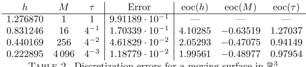
6.3. Moving surface. We consider the ellipsoid
Γ(t) =
x= (x1, x2, x3)∈R3
x2 1 a(t)+x
2 2+x
2 3= 1
Figure 1. Polygonal approximation Γh,0 of Γ(0) forh=h0, . . . , h4.
h M τ Error eoc(h) eoc(M) eoc(τ)
1.500000 1 1 3.00350 — — —
0.843310 16 4−1 2.23278·10−1 4.51325 −0.93743 1.87487 0.434572 256 4−2 1.86602·10−1 0.27066 −0.06472 0.12944 0.218962 4 096 4−3 4.88096·10−2 1.95642 −0.48368 0.96736 0.109692 65 536 4−4 1.29667·10−2 1.91768 −0.47809 0.95618
Table 1. Discretization errors for a moving curve inR2.
with oscillating x1-axis a(t) = 1 + 14sin(t) and T = 1. The random diffusion
coefficientαoccurring inah(·,·) is given by
α(x, ω) = 1 +x21+Y1(ω)x41+Y2(ω)x42,
where Y1 and Y2 denote independent, uniformly distributed random variables on
Ω = (−1,1). The right-hand side f in (6.1) is chosen such that for eachω∈Ω the exact solution of the resulting path-wise problem is given by
u(x, t, ω) = sin(t)x1x2+Y1(ω) sin(2t)x21+Y2(ω) sin(2t)x2,
and we setu0(x, ω) =u(x,0, ω) = 0.
The initial triangular approximation Γh,0of Γ(0) is depicted in Figure6.3for the
[image:23.612.149.460.580.649.2]mesh sizesh=hj,j= 0, . . . ,3. We select the corresponding time step sizesτ0= 1,
Figure 2. Triangular approximation Γh,0 of Γ(0) forh=h0, . . . , h3.
h M τ Error eoc(h) eoc(M) eoc(τ)
1.276870 1 1 9.91189·10−1 — — —
0.831246 16 4−1 1.70339·10−1 4.10285 −0.63519 1.27037 0.440169 256 4−2 4.61829·10−2 2.05293 −0.47075 0.94149 0.222895 4 096 4−3 1.18779·10−2 1.99561 −0.48977 0.97954
Table 2. Discretization errors for a moving surface inR3.
we observe that the discretization error behaves likeO(h2+M−1/2+τ). This is in accordance with our theoretical findings stated in Theorem 5.5and fully discrete deterministic results [18, Theorem 2.4].
References
[1] A. Alphonse, C. M. Elliott, and B. Stinner. An abstract framework for parabolic PDEs on evolving spaces. Port. Math., 72(1):1–46, 2015. doi: 10.4171/pm/1955.
[2] A. Alphonse, C. M. Elliott, and B. Stinner. On some linear parabolic PDEs on moving hypersurfaces. Interfaces Free Bound., 17(2):157–187, 2015. doi: 10.4171/ifb/338.
[3] A. Barth, Ch. Schwab, and N. Zollinger. Multi-level Monte Carlo finite element method for elliptic pde’s with stochastic coefficients. Numer. Math., 119(1): 123–161, 2011. doi: 10.1007/s00211-011-0377-0.
[4] P. Bastian, M. Blatt, A. Dedner, C. Engwer, R. Kl¨ofkorn, M. Oldberger, and O. Sander. A generic grid interface for parallel and adaptive scientific comput-ing. Part I: Abstract framework. Computing, 82:103–119, 2008.
[5] P. Bastian, M. Blatt, A. Dedner, C. Engwer, R. Kl¨ofkorn, M. Oldberger, and O. Sander. A generic grid interface for parallel and adaptive scientific com-puting. Part II: Implementation and tests inDune. Computing, 82:121–138, 2008.
[6] M. Bertalm´ıo, Li-Tien Cheng, S. J. Osher, and G. Sapiro. Variational problems and partial differential equations on implicit surfaces. J. Comput. Phys., 174 (2):759–780, 2001. ISSN 0021-9991.
[7] J. Charrier. Strong and weak error estimates for elliptic partial differential equations with random coefficients. SIAM J. Numer. Anal., 50(1):216–246, 2012. doi: 10.1137/100800531.
[8] J. Charrier. Numerical analysis of the advection-diffusion of a solute in porous media with uncertainty. SIAM/ASA J. Uncertain. Quantif., 3(1):650–685, 2015. doi: 10.1137/130937457.
[9] J. Charrier, R. Scheichl, and A. L. Teckentrup. Finite element error analysis of elliptic pdes with random coefficients and its application to multilevel Monte Carlo methods. SIAM J. Numer. Anal., 51(1):322–352, 2013. doi: 10.1137/ 110853054.
[10] A. Cliffe, M. Giles, R. Scheichl, and A. L. Teckentrup. Multilevel Monte Carlo methods and applications to elliptic pdes with random coefficients. Comput.
Vis. Sci., 14(1):3–15, 2011. doi: 10.1007/s00791-011-0160-x.
[11] K. Deckelnick, G. Dziuk, and C. M. Elliott. Computation of geometric partial differential equations and mean curvature flow. Acta Numer., 14:139–232, 2005. doi: 10.1017/s0962492904000224.
[12] A. Dedner., R. Kl¨ofkorn, M. Nolte, and M. Ohlberger. A generic interface for parallel and adaptive discretization schemes: abstraction principles and the Dune-Fem module. Computing, 90(3-4):165–196, 2010. doi: 10.1007/ s00607-010-0110-3.
[14] A. Djurdjevac. Advection-diffusion equations with random coefficients on evolving hypersurfaces. Technical report, Freie Universit¨at Berlin ( to appear in Interfaces and Free Boundaries), 2015.
[15] G. Dziuk. Finite elements for the Beltrami operator on arbitrary surfaces. In S. Hildebrandt and R. Leis, editors,Partial differential equations and calculus
of variations, volume 1357 of Lecture Notes in Mathematics, pages 142–155.
Springer, Berlin, Heidelberg, 1988.
[16] G. Dziuk and C. M. Elliott. Finite elements on evolving surfaces. IMA J.
Numer. Anal., 27(2):262–292, 2006. doi: 10.1093/imanum/drl023.
[17] G. Dziuk and C. M. Elliott. L2-estimates for the evolving surface
fi-nite element method. Math. Comp., 82(281):1–24, 2012. doi: 10.1090/ s0025-5718-2012-02601-9.
[18] G. Dziuk and C. M. Elliott. A fully discrete evolving surface finite ele-ment method. SIAM J. Numer. Anal., 50(5):2677–2694, 2012. doi: 10.1137/ 110828642.
[19] G. Dziuk and C. M. Elliott. Finite element methods for surface PDEs. Acta
Numer., 22:289–396, 2013. doi: 10.1017/s0962492913000056.
[20] C. M. Elliott and T. Ranner. Evolving surface finite element method for the Cahn-Hilliard equation. Numer. Math., 129(3):483–534, 2014. doi: 10.1007/ s00211-014-0644-y.
[21] C. M. Elliott, B. Stinner, and C. Venkataraman. Modelling cell motility and chemotaxis with evolving surface finite elements.J. R. Soc. Interface, 82, 2012. doi: doi:10.1098/rsif.2012.0276.
[22] W. Hackbusch. Tensor Spaces and Numerical Tensor Calculus. Springer. Berlin, Heidelberg, 2012. doi: 10.1007/978-3-642-28027-6.
[23] P. R. Halmos. Measure Theory. Graduate Texts in Mathematics. Springer, 1976.
[24] L. Herrmann, A. Lang, and Ch. Schwab. Numerical analysis of lognormal diffusions on the sphere. arXiv:1601.02500v2, 2016.
[25] V. H. Hoang and Ch. Schwab. Sparse tensor galerkin discretization of para-metric and random parabolic PDEs—analytic regularity and generalized poly-nomial chaos approximation. SIAM J. Math. Anal., 45(5):3050–3083, 2013. doi: 10.1137/100793682.
[26] H. Jin, T. Yezzi, and J. Matas. Region-based segmentation on evolving surfaces with application to 3d reconstruction of shape and piecewise constant radiance.
In Computer Vision - ECCV 2004: 8th European Conference on Computer
Vision, Proceedings, Part II, pages 114–125. Springer Berlin Heidelberg, 2004.
doi: 10.1007/978-3-540-24671-8 9.
[27] R. Kornhuber and H. Yserentant. Multigrid methods for discrete elliptic prob-lems on triangular surfaces. Comp. Vis. Sci., 11(4-6):251–257, 2008.
[28] S. Larsson, C. Mollet, and M. Molteni. Quasi-optimality of Petrov-Galerkin discretizations of parabolic problems with random coefficients. arXiv:1604.06611, 2016.
[29] G. Lord, C. E. Powell, and T. Shardlow. An Introduction to Computational
Stochastic PDEs. Cambridge University Press, 2014.
[31] O. P. Le Maˆıtre and O. M. Knio. Spectral Methods for Uncertainty
Quantifi-cation. Springer Netherlands, 2010. doi: 10.1007/978-90-481-3520-2.
[32] N. R. Morrow and G. Mason. Recovery of oil by spontaneous imbibition.
Current Opinion in Colloid and Interface Science, 6(4):321–337, 2001. doi:
10.1016/S1359-0294(01)00100-5.
[33] F. Nobile and R. Tempone. Analysis and implementation issues for the nu-merical approximation of parabolic equations with random coefficients.Int. J.
Numer. Meth. Engng., 80(6-7):979–1006, 2009. doi: 10.1002/nme.2656.
[34] R.G. Plaza, F. S´anchez-Gardu˜no, P. Padilla, R.A. Barrio, and P.K. Maini. The effect of growth and curvature on pattern formation. J. Dynamics and
Differential Equations, 16:1093–1121, 2004.
[35] M. Reed and B. Simon. Methods of modern mathematical physics. vol. 1.
Functional analysis. Academic, New York, 1980.
[36] A. Reusken and M.A. Olshanskii. Trace finite element methods for PDEs on surfaces. arXiv:1612.0005, 2016.
Institut f¨ur Mathematik, Freie Universit¨at Berlin, 14195 Berlin, Germany
E-mail address:[email protected]
Mathematics Institute, University of Warwick, Coventry. CV4 7AL. UK
E-mail address:[email protected]
Institut f¨ur Mathematik, Freie Universit¨at Berlin, 14195 Berlin, Germany
E-mail address:[email protected]
School of Computing, University of Leeds, Leeds. LS2 9JT. UK