PSS for various electromechanical

Abstract— Power systems stabilizers (PSS) are very effective

for damping oscillation due to occurring disturbances and keeping synchronism in excitation circuits of synchronous generators. Design and tuning of PSS are crucial issues for researchers involved in the development of power systems control . It is because of inaccurate setting of PSS that not only it causes damping oscillations but it also contributes to the amplification of instability leading to the loss of synchronism. In this paper, an optimum PSS is designed using a novel method called combinatorial discrete and continuous action reinforcement learning automata (CDCARLA). The proposed method is implemented for a single machine-infinite bus (SMIB) and it is compared with an IEEE standard PSS. Simulation results show that the proposed PSS has a significantly better performance as well as satisfactory robustness compared to the standard PSS. The advantage of CDCARLA is that it does not need system dynamics or any other information on power system. It can be said that, this method utlizes nonlinear features of power system. The CDCARLA method can be considered as one of the automatic design techniques using PSS.

Index Terms— Power system stabilizer, Reinforcement

learning automata, SMIB, Transient stability

1. INTRODUCTION

Due to increasing complexity of electric power systems, there is significant interests in the stabilization of such systems. Power system stabilizers(pss) are the most effective devices for stabilizing and damping low frequency oscillations, while increasing the stability margin of power systems [1]. A PSS prepares a supplementary input signal in-phase with the synchronous rotor speed deviations to excitation systems resulting in generator stability.

In the last two decades, various types of PSS have been designed. For example, conventional power system stabilizers (CPSS) are composed of fixed lag-lead compensators and they are widely used in power systems [2]. Adaptive controller-based PSS have been used in many applications [3-4]. However, most of these controllers are based on system identification and parameter estimation; therefore from computational point of view they are time consuming. It is evident from the various publications that interest in applications of Fuzzy logic based PSS (FLPSS) has also grown in recent years [5-8].

Low computation burden, simplicity and robustness make FLPSS suitable for stabilization purposes. Different methods for designing such devices are proposed using genetic

1. Shahid Bahonr University of Kerman,Keman,Iran 2. Shahrood University of Technology, Iran 3. London Metropolitan University, UK

algorithm (GA) [9] and artificial neural networks (ANN) [10].

In this paper, a novel design method based on Reinforcement Learning Automata (RLA) is proposed. The methodology employed for designing PSS involves two major stages. In the first stage, the best variation limits of controller parameters are obtained using discrete action reinforcement learning automata (DARLA). In the second stage, the best value of these parameters in a pre-specified limit is determined. In fact, the second stage was proposed originally by Howell et. al. [11] for a vehicle suspension control application in 1997 and named as the combinatorial discrete and continuous action reinforcement learning automata

(CARLA). One of the major advantages of CARLA is high speed convergence; while it requires pre-specified decision variables variation limits. These limits can be obtained by using any simple method such as local linearization. CARLA requires system dynamics in the initial step which can be considered as one of its main disadvantage. Moreover, system equations can not be achieved easily for any application. DARLA has similar properties as CARLA such as fast convergence, system dynamics independency and nonlinear characteristic. The proposed method is based on combination of both DARLA and CARLA and it is called combined discrete and continuous action reinforcement learning automata (CDCARLA) with the all of above desirable properties. For evaluating the performance of CDCARLA design, a PSS is designed and its stabilization behavior is simulated and compared with IEEE standard PSS for a single machine infinite bus. Simulation results show that the proposed method has a better performance in comparison with standard PSS for various electromechanical disturbances.

In the following sections, power system modeling techniques used is first described. The coverage of the design methodology and the two major stages involved are then dealt with in section 3. Simulation and related results are described in section 4 and finally the paper ends with conclusion in section 5.

2. POWER SYSTEM MODELING

The block diagram for the designed conventional PSS is shown in Fig. 1.

Fig.1. Conventional .Power System Stabilizer

Note that the PSS excitation signal is the only output variable that leads to PSSou. while it has five unknown variables.

A Novel Automatic Designing Technique for

Tuning Power System Stabilizer

SMIB MODEL

A single machine infinite bus (SMIB) model of a power system for evaluating the proposed design method is considered. Using this model, we consider a typical 500MVA, 13.8 kV, 50Hz synchronous generator together with a 500MVA, 13.8/400kV transformer and a 400kv, 350 km transmission line connected to an infinite bus. Single line diagram of the model is shown in Fig. 2 [15].

G

Synchronous Generator 500 MVA, 13.8 KV, 50 Hz

Power Transformer 500 MVA, 13.8/400 KV, 50 Hz

Power Transmission Line 400 KV, 350 Km, 50 Hz

Infinite Bus

[image:2.595.51.289.158.209.2]

Network 10,000 MVA, 400 KV, 50 Hz Power Plant Bus

Fig. 2. Single line diagram of SMIB model

Fig 3 shows a generation unit consisting of a synchronous generator, a turbine, a governor, an excitation system, an automatic voltage regulator (AVR) and a PSS.

Synchronous Generator

Turbine Δω

Governor

+ _ PRef

Exciter AVR

+ +

VTRef

VT

VA

PSS VS +

P

Δ ω Δ / TM

PSV

Fig. 3. Generation unit diagram

Next, a transient model of a synchronous machine is considered and its mechanical parts are modeled by;

0 0

) ( ) (

) ( )

( 2

1 ) (

ω + ω Δ = ω

ω Δ − − =

ω

Δ

_∫

t t

t K dt T T H

t _d

t

E

M (1)

(2) Where, Δω is speed variation, ω is mechanical speed of rotor, H is the inertia constant, T_M / T_E are mechanical /

electrical torque respectively and K_d is a damping factor.

Electrical parts of synchronous machine can be described by a sixth order state space model. Table 3 in the Appendix show the synchronous generator parameters.

[image:2.595.318.522.221.379.2]

A nonlinear model [12] for hydraulic turbine and governor shown in Fig 4 is used to for the SMIB power system. Hydraulic turbine and governor parameters are presented in the Appendix (table 4).

Fig. 4. Turbine and Governor model

AVR and excitation system are modeled based upon IEEE standard 421.5 [13] and their parameters are reported in the Appendix (Table 5).

Mathematical model for the power transformer considers core saturation, core and winding losses and leakage flux. Equivalent circuit parameters of power transformer are also shown in the Appendix (table 6).

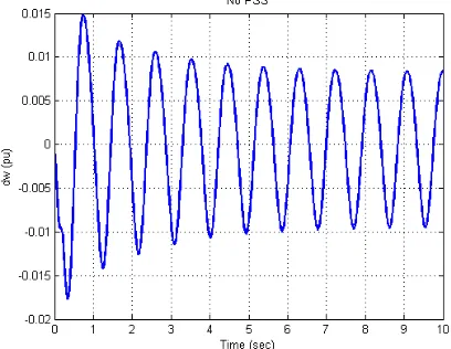
[image:2.595.68.269.283.404.2]

Mathematical model for transmission line that implements lumped losses is based on Bergeron traveling wave method [14]. Open loop response of rotor speed variation is shown in Fig. 5.

Fig.5. Rotor speed deviation for single earth fault (no control)

3. DESIGN METHODOLOGY

The proposed design methodology is based on Reinforcement Learning Automata (RLA) and has two stages. First stage is based on discrete action and determines the best variation limits for each coefficient (DARLA). Second stage searches the best value of each parameter that is specified at previous stage (CARLA). The key idea of DARLA and CARLA is that, if a value of decision variable results in a good performance for a system, then closed values for decision variable have probably a relative good performance. Both methods use probability distribution function (PDF) through changing for sufficient time in order to obtain an optimal value for decision variables.

Design Stage : DARLA

In DARLA, the variation limits of controller coefficients are usually divided into the same length limits. Then a discrete probability distribution function (DPDF) for each of those limits will be assigned in which DPDFs initially set as a uniform type. The probability of selecting each limit is performed by DPDF, while after each selection the shape of DPDFs is changed in proportion to the fitness of that selection. Fig. 6 shows a block diagram of DARLA method. GT

2 ⎟⎟ ⎠ ⎞ ⎜⎜ ⎝ ⎛

w

G G

Σ

+

β

ω Δ

_

Σ

+ _ 1

w T

1 ∫

x

Turbine Gain G Gw

TM

Hydraulic Turbine PID

Σ

wRef

we

+

Σ

Σ

PRef

Pe

+ RP

Permanent Droop _

+ _

_ Σ +

1

+

s T

k

A A

Servo Motor

∫ Speed Limit

Position Gate _

[image:2.595.51.251.655.751.2]

Updating DPDF by Reinforcement Signal β

Reinforcement Signal For Selected Limits Cost J

Reinforcement Signal β Selecting Limits

By DPDF

[image:3.595.65.273.50.170.2]

Selected Limits _{TSFLPSS and} Power System

Fig. 6. DARLA workflow

PSS should be able to turn back this system to stable conditions (Δω=0) at a minimum time. A training power system is shown in Fig. 7 in which a single earth fault occurs at 0.1 sec in phase A and it is cleared at 0.2 sec.

G Infinite Bus

Power Plant Bus

Generator

Singke Phase Earth Fault On Phase A @ 0.1 sec

[image:3.595.72.268.235.308.2]

And Cleared @ 0.2 sec

Fig. 7. Training power system diagram

As it is stated, there are 5 controller coefficients and let assume each variable varies between -10 and 10. This limit is divided into 20 equal divisions. Number of divisions does not severely affect the design performance, yet its selected value must be large enough. As a result, we have 6 DPDFs with 20 elements that initially defined as Eq. (3).

27 , , 2 , 1 0 20 , , 2 , 1 )

( 201 ) 0 ( L L = ⎩ ⎨ ⎧ = = i otherwise n n f_i (3) Where ( )( )

p

fik is the probability of selecting pth limit in ith

controller coefficients at kth iteration.

After selecting limits by cumulative probability of DPDFs, center of each limit is taken to construct the proposed PSS and J cost function is calculated based on Eq. (4).

SS t T k G G dt G

J =

∫

Δ

ω

+ 2 Δ

ω

+ 3Δ

ω

0

1 )

( _sup

(4) where J(k) _{is cost function at kth iteration, T is simulation time}

that must be large enough (for example T=3sec_{), Δω is rotor}

speed deviation, ΔωSS is steady state error of speed deviation,

G1, G2 and G3 are cost function weights. After calculating cost

function, reinforcement signal β is calculated using Eq. (5).

⎭ ⎬ ⎫ ⎩ ⎨ ⎧ ⎭ ⎬ ⎫ ⎩ ⎨ ⎧ − − = β min ) ( )

( _{min 1,max 0,}

J J J J mean k mean k (5) Where β(k) _{is kth reinforcement signal, and J}

mean and Jmin are

average and minimum of previous costs, respectively. Defining reinforcement signal as Eq. (5) gives the average of costs with non-increasing behavior that guarantees convergence.

After obtaining reinforcement signal, DPDFs are updated by Eq. (6).

(

() () ()

)

) ( ) 1

( _{( ) ( )} k

i k k i k i k

i n f n Q

f + =α +β (6)

Where (k) i

Q is an exponential function centered in selected

limit and defined as Eq. (7). 2

) ~ ( )

( ₂ n ni

q k i r

Q = − − (7)

Note n~_ia is the selected limit and rq is is a positive constant. )

(k i

α in Eq. (6) is a normalization factor calculated by Eq.(8).

∑

= β + = α ₂₀ 1 ) ( ) ( ) ( ) ( ) ( 1 n k i k k i k i Q n f (8)

After sufficient iterations, the selection probability of optimal limit for each DPDF is maximized. Fig. 8 shows discrete convergence surface of one of the controller coefficients for 100 iterations with the following parameters:

401 3

2

1=10,G =100,G =500,rq = G

[image:3.595.317.523.256.683.2]

Fig. 9 shows the cost variations versus number of iterations. As it is expected a non-increasing behavior can be seen. The limit with highest probability of selection at the end of iterations for each of controller coefficient is the optimum limit for the corresponding coefficient. These intervals are shown in Table 1.

Fig 8. Convergence surface for coefficient T1

0 20 40 60 80 100

0 5 10

15x 10

4

Iterations C

ost

Cost Variation

Fig. 9. Cost variation of DARLA design stage

Table 1. Optimum interval of coefficients

Parameter Optimum Interval Ks [9,10] T1 [5,6] T2 [2,3] T3 [0,1] T4 [1,2]

Design Stage 2: CARLA

The mathematical relations for calculating cost and reinforcement signal is the same as DARLA and they are given by equations (4) and (5). CPDF updating rule is a little different and is performed by Eq. (9).

(

)

i

k i k k

i k i k

i

X x i

H x f x

f

∈ =

β + α

=

+

; 27 , , 2 , 1

) ( )

( () () () () )

1 (

L (9)

Where f(x) is CPDF, Xi is an optimum limit and H is

exponential function centered on the selected coefficient value defined by Eq. (10).

⎟⎟ ⎠ ⎞ ⎜⎜

⎝

⎛ −

− =

w i h

k i

g x x g

H

2 ) ~ ( exp

2 )

(

(10) Note gh and gw are height and width of exponential function,

respectively. (k) i

α in equation (9) is a normalization factor calculated as shown in Eq.(11).

∫

∈

β + =

α

i X x

k i k k

i k i

dx H x

f() () () )

(

) (

1

(11) By carrying out enough iteration of the above steps, the CARLA method will converge to an optimum value for each controller coefficient in an optimal limit. Fig. 10 shows continuous convergence surface of one of the controller coefficients for 100 iterations with the following parameters:

9 . 0 , 003 . 0 , 500 ,

100 ,

10 2 3

1= G = G = gw= gh=

G

Fig10. Convergence surface for coefficient T1

The variation of cost versus iterations is shown in Fig. 11. The limit with highest probability of selection at the end of iterations for each of controller coefficient is the optimum limit for the corresponding coefficient. These values are shown in Table 2.

0 10 20 30 40 50 60 70 80 90 100

0 200 400 600 800

Iterations C

ost

[image:4.595.353.499.61.141.2]

CARLA Cost Variation

Fig 11. Variation of CARLA cost function due to iterations

Table 2. Optimum Value of coefficients

Paramete r

Optimum Value

Ks 9.6693

T1

5.988

T2

2.0541

T3

0.0561

T4

1.0902

4. SIMULATION AND RESULTS

In this section, performance of designed controller is evaluated and compared with IEEE conventional PSS from IEEE standard 421.5 [15]. The simulations carried out using MATLAB® and SIMULINK® environment for training system Fig. 6. For evaluating robustness of proposed PSS stabilizations of these PSSs is simulated for other different types of disturbances.

4.1 Design Performance Evaluation

[image:4.595.333.512.338.630.2]

Fig. 12 shows rotor speed deviation of single phase earth fault on a generator bus at two situations: proposed PSS (Optimum PSS) and conventional PSS. Fig. 13 also shows line power variations for different PSS.

Fig 12. Rotor speed deviation for single earth fault

Fig. 13. Line power variations for single earth fault

It can be seen in figures 12, 13, the optimum PSS (OPSS) designed by the proposed method has better performance than that of the conventional PSS in damping low frequency oscillation.

4.2. Robustness Evaluation

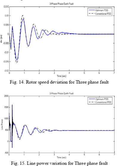
[image:4.595.55.273.644.729.2]

[image:5.595.324.528.51.674.2]

above disturbances for different types of PSSs are drawn in Fig. 14 and Fig. 15.

Fig. 14. Rotor speed deviation for Three phase fault

Fig. 15. Line power variation for Three phase fault

Note that the proposed PSS is relatively more robust and more effective than other PSS types due to various power disturbances. For comparing stabilization performance of different PSSs the following two properties of rotor speed deviation have been considered:

• Required time for complete system stabilization (Δω=0)

• Maximum magnitude of rotor speed deviation Both of these properties are measured after transient period of synchronous machine and they can be selected as stabilization performance index.

5. CONCLUSIONS

In this paper, a novel heuristic design method for a conventional power system stabilizer, called CDCARLA, is proposed. This method is based upon reinforcement learning automata and does not require system dynamics or any further information. In comparison with the other heuristic search methods such as Genetic Algorithm and Particle Swarm Optimization (PSO), CDCARLA converges in very little iteration. In addition, the proposed design method does not ignore any nonlinear feature of power systems. Simulation results prove a better performance and design robustness of the proposed algorithm. In summary, CDCARLA can be used as a good automatic design method for a wide range of applications.

6. APPENDIX

Table 3. Synchronous machine parameter

Parameter Value

Rotor Type Salient-pole

Number of Poles 64

Nominal Power 500 MVA

Line to Line Voltage (RMS) 13.8 kV

Frequency 50 Hz

Reactances (pu)

Xd 1.305

X’

d 0.296

X”

d 0.252

Xq 0.474

X”

q 0.283

XI 0.18

Time Constants (s) T’

d 1.01

T”

d 0.053

T”

q0 0.1

Stator Resistance (pu) 0.0028544

Inertia Factor 3.7

[image:5.595.326.526.72.673.2]

Friction Factor 0

Table 4. Hydraulic turbine and governor parameters

Parameter Value

Governor

Permanent Droop 0.05

Servo Motor

KA 3.33

TA (s) 0.07

Speed Limit (pu) [-0.1,0.1]

PID Regulator

KP 1.163

KI 0.105

KD 0.01

Hydraulic Turbine

Β 0

TW (s) 2.67

GT 1

Table 5. AVR and excitation system parameters

Parameter Value

Low pass Filter Time Constant (TR) 0.002

Regulator

Gain (KA) 200

Time Constant (TA) 0.001

Exciter

Gain (KE) 1

Time Constant (TE) 0

Lag-Lead Compensator

TB 0

TC 0

Damping Filter

Gain (KF) 0.001

Time Constant (TF) 0.1

Table 6. Power transformer parameters

Parameter Value

Nominal Power 500 MVA

Frequency 50 Hz

Winding 1

Connection Δ

Phase-Phase Voltage (RMS) 13.8 kV

Resistance (pu) 0.002

Inductance (pu) 0

Winding 2

Connection Y

Phase-Phase Voltage (RMS) 400 kV

Resistance (pu) 0.002

Inductance (pu) 0.12

Magnetizing Resistance (pu) 500

Magnetizing Reactance (pu) 500

7. Acknowledgements

[image:5.595.69.267.73.351.2]

REFERENCES

[1] P. M. Anderson and A. A. Fouad, Power System Control and Stability,

Iowa State University Press, Iowa, U.S.A., 1997.

[2] E. Larsen and D. Swann, “Applying Power System Stabilizers,” IEEE

Transaction PAS, Vol. 100, No. 6., 1981, pp. 3017-3046.

[3] J. J. Dai and A. A. Ghandakly, “A Decentralized Adaptive Control Algorithm and the Application in Power System Stabilizer (PSS) Design,” 1997

[4] R. Segal, M. L. Kothari and S. Madnani, “Radial Basis Function (RBF) Network Adaptive Power System Stabilizer,” IEEE Transactions on

Power Systems, Vol. 15, May 2000, pp. 722-727.

[5] N. Nallathambi, P. N. Neelakantan, “Fuzzy Logic Based Power System Stabilizer,” in Proceeding 2004 E-Tech Conference, pp. 68-73.

[6] N. Hosseinzadeh and A. Kalam, “A Direct Adaptive Fuzzy Power System Stabilizer,” IEEE Transactions on Energy Conversion, Vol. 14, Dec 1999, pp. 1564-1571.

[7] P. Hoang and K. Tomsovic, “Design And Analysis Of An Adaptive Fuzzy Power System Stabilizer,” IEEE Transactions on Energy

Conversion, Vol. 455-461, June 1996.

[8] T. Hiyama, M. Kugimiya and H. Satoh, “Advanced PID Type Fuzzy Logic Power System Stabilizer,” IEEE Transactions on Energy

Conversion, Vol. 9, Sep 1994, pp. 514-520.

[9] M. A. Abido and Y. L. Abdel-Magid, “A Genetic-Based Fuzzy Logic Power System Stabilizer For Multimachine Power Systems,” in

Proceeding of 1997 IEEE International Conference on Computational

Cybernetics and Simulation Systems, pp. 329-334.

[10] A. Hariri, O. P. Malik, “Adaptive-Network-Based Fuzzy Logic Power System Stabilizer,” in Proceeding of 1995 Communications, Power, and

Computing Conference, pp. 111-116.

[11] M. N. Howell, G. P. Frost, T. J.Gordon and Q. H. Wu, “Continuous Action Reinforcement Learning Applied to Vehicle Suspension Control,” Mechatronics, 1997, pp. 263-276.

[12] IEEE Working Group on Prime Mover and Energy Supply Models for System Dynamic Performance Studies, “Hydraulic Turbine and Turbine Control Models for Dynamic Studies,” IEEE Transactions on Power

Systems, Vol. 7, Feb 1992, pp. 167-179.

[13] Recommended Practice for Excitation System Models for Power System

Stability Studies, IEEE Standard 421.5-1992, August, 1992.

[14] H. Dommel, “Digital Computer Solution of Electromagnetic Transients in Single and Multiple Networks,” IEEE Transactions on Power

Apparatus and Systems, Vol. PAS-88, April 1969.

[15] N. Martins, A.A. Barbosa, J.C.R. Ferraz, M.G. dos Santos, A.L.B. Bergamo, C.S. Yung, V.R. Oliveira, and N.J.P. Macedo, “Retuning

Stabilizersfor the North-South Brazilian Interconnection, “ IEEE PES

SummerMeeting, 18-22 July 1999 , Vol. 1, pp. 58–67.

[16] R. Grondin, I. Kamwa, G. Trudel, L. Gérin-Lajoie, and J. Taborda, “Modelingand Closed-Loop Validation of a New PSS Concept, The Multi-BandPSS,” Presented at the 2003 IEEE/PES General Meeting, Panel Sessionon New PSS Technologies, Toronto, Canada