http://wrap.warwick.ac.uk
Original citation:
Rubio, Francisco J. and Johansen, Adam M.. (2013) A simple approach to maximum
intractable likelihood estimation. Electronic Journal of Statistics, Volume 7 . pp.
1632-1654. ISSN 1935-7524
Permanent WRAP url:
http://wrap.warwick.ac.uk/63809
Copyright and reuse:
The Warwick Research Archive Portal (WRAP) makes this work of researchers of the
University of Warwick available open access under the following conditions.
This article is made available under the Creative Commons Attribution 2.5 Licence (CC
BY 2.5) and may be reused according to the conditions of the license. For more details
see: http://creativecommons.org/licenses/by/2.5/
A note on versions:
The version presented in WRAP is the published version, or, version of record, and may
be cited as it appears here.
Vol. 7 (2013) 1632–1654 ISSN: 1935-7524 DOI:10.1214/13-EJS819
A simple approach to
maximum intractable likelihood
estimation
F. J. Rubio∗ and Adam M. Johansen†
University of Warwick, Department of Statistics, Coventry, CV4 7AL, UK e-mail:[email protected];[email protected]
Abstract: Approximate Bayesian Computation (ABC) can be viewed as
an analytic approximation of an intractable likelihood coupled with an elementary simulation step. Such a view, combined with a suitable in-strumental prior distribution permits maximum-likelihood (or maximum-a-posteriori) inference to be conducted, approximately, using essentially the same techniques. An elementary approach to this problem which simply ob-tains a nonparametric approximation of the likelihood surface which is then maximised is developed here and the convergence of this class of algorithms is characterised theoretically. The use of non-sufficient summary statistics in this context is considered. Applying the proposed method to four prob-lems demonstrates good performance. The proposed approach provides an alternative for approximating the maximum likelihood estimator (MLE) in complex scenarios.
Keywords and phrases:Approximate Bayesian Computation, density
estimation, maximum likelihood estimation, Monte Carlo methods.
AMS 2000 subject classifications:62E17, 62F10, 62F12, 62G07, 65C05.
Received January 2013.
Contents
1 Introduction . . . 1633
2 Approximate Bayesian Computation . . . 1635
3 Maximising intractable likelihoods . . . 1636
3.1 Algorithm . . . 1636
3.2 Asymptotic behaviour . . . 1637
3.3 Use of kernel density estimators . . . 1644
4 Examples . . . 1644
4.1 Binomial model . . . 1644
4.2 Normal model . . . 1646
4.3 α-stable logarithmic daily returns model . . . 1646
4.4 Superposed gamma point processes . . . 1648
5 Discussion . . . 1651
Acknowledgements . . . 1652
References . . . 1652
∗FJR acknowledges support from Conacyt, M´exico.
†AMJ gratefully acknowledges support from EPSRC grant EP/I017984/1.
1. Introduction
Modern applied statistics must deal with many settings in which the point-wise evaluation of the likelihood function, even up to a normalising constant, is impossible or computationally infeasible. Areas such as financial modelling, genetics, geostatistics, neurophysiology and stochastic dynamical systems pro-vide numerous examples of this (see e.g. Cox and Smith,1954; Pritchard et al., 1999; and Toni et al.,2009). It is consequently difficult to perform any inference (classical or Bayesian) about the parameters of the model. Various approaches to overcome this difficulty have been proposed. For instance, Composite Likelihood methods (Cox and Reid,2004), for approximating the likelihood function, and Approximate Bayesian Computational methods (ABC; Pritchard et al., 1999; Beaumont et al.,2002), for approximating the posterior distribution, have been extensively studied in the statistical literature. Here, we study the use of ABC methods, under an appropriate choice of the instrumental prior distribution, to approximate the maximum likelihood estimator.
It is well-known that ABC produces a sample approximation of the poste-rior distribution (Beaumont et al., 2002) in which there exists a deterministic approximation error in addition to Monte Carlo variability. The quality of the approximation to the posterior and theoretical properties of the estimators ob-tained with ABC have been studied in Wilkinson (2008); Blum (2010); Marin et al. (2011); Dean et al. (2011); and Fearnhead and Prangle (2012). The use of ABC posterior samples for conducting model comparison was studied in Dide-lot et al. (2011) and Robert et al. (2011). Using this sample approximation to characterise the mode of the posterior would in principle allow (approximate) maximum a posteriori (MAP) estimation. Furthermore, using a uniform prior distribution, under the parameterisation of interest, over any set which contains the MLE will lead to a MAP estimate which coincides with the MLE. This is an immediate consequence of Bayes’ Theorem. In low-dimensional problems if we have a sample from the posterior distribution of the parameters, we can estimate its mode by using either nonparametric estimators of the density or another mode–seeking technique such as the mean-shift algorithm (Fukunaga and Hostetler,1975). Therefore, in contexts where the likelihood function is in-tractable we can use these results to obtain an approximation of the MLE. We will denote the estimator obtained with this approximation AMLE.
of unknown parameters and latent states are available — not a requirement of the more general ABC technique developed below. The same idea was ap-plied and analysed in the context of the estimation of location parameters, with particular emphasis on symmetric distributions, by Jaki and West (2008).
Bret´o et al. (2009) proposed the plug-and-play technique which permits con-ducting likelihood-based inference, despite the complexity of the corresponding likelihood function, on time series models which allow for simulating realisations at any parameter values. The particular case of parameter estimation in hidden Markov models was also investigated by Dean et al. (2011), whose approach relies upon the specific structure of Markov models (essentially the standard particle filtering estimate of the likelihood for a modified model is employed) and an attempt to numerically optimise the likelihood using these Monte Carlo point estimates is made. They note that even in simple univariate models the simulation cost can be rather high. Their approximation (denoted ABC MLE) can be interpreted as a maximum likelihood estimation of a misspecified model. At the cost of some loss of efficiency the bias introduced by the use of finite tolerance can be eliminated by a noisy ABC (Fearnhead and Prangle, 2012) argument.
Another approach to estimation in intractable models is provided by the
indirect inference approach of Gouri´eroux et al. (1993), but this approach re-quires the introduction of an explicit proxy model and a relationship between the parameters of the original model and its proxy to be specified.
To the best of our knowledge neither MAP estimation nor maximum likeli-hood estimation in general, implemented directly via the “ABC approximation” combined with maximisation of an estimated density, have been studied in the literature. However, there has been a lot of interest in this type of problem using different approaches (Cox and Kartsonaki,2012; Ehrlich et al.,2012; Fan et al., 2012; Mengersen et al., 2013; and Biau et al.,2012who establish a number of results including one closely related to our Proposition1in settings in which a particular post-simulation approach to the specification of the tolerance param-eter is adopted) since we completed the first version of this work (Rubio and Johansen,2012).
The use of the mode of a nonparametric kernel density estimate to estimate the mode of a density, which may seem, at first, to be a hopeless task has also received a lot of attention (see e.g. Parzen,1962; Konakov,1973; Romano,1988; Abraham et al., 2003; Bickel and Fr¨uwirth, 2006). Alternative nonparametric density estimators which could also be considered within the AMLE context have been proposed recently in Cule et al. (2010); Jing et al. (2012).
2. Approximate Bayesian Computation
We assume throughout this and the following section that all distributions of interest admit densities with respect to an appropriate version of Lebesgue measure, wherever this is possible, although this assumption can easily be re-laxed. Let x= (x1, . . . , xn)∈Rq×n be a sample with joint distribution f(·|θ),
θ ∈Θ⊂Rd; L(θ;x) be the corresponding likelihood function,π(θ) be a prior distribution over the parameterθ and π(θ|x) the corresponding posterior dis-tribution. Consider the following approximation to the posterior
b
πε(θ|x) = b
fε(x|θ)π(θ) R
Θfbε(x|t)π(t)dt
, (1)
where
b
fε(x|θ) = Z
Rq×n
Kε(x|y)f(y|θ)dy, (2)
is an approximation of the likelihood function and Kε(x|y) is a normalised
Markov kernel. Kε(·|y) is typically concentrated around y with ε acting as a
scale parameter. It is clear that (2) is a smoothed version of the true likelihood and it has been argued that the maximisation of such an approximation can in some circumstances lead to better performance than the maximisation of the likelihood itself (Ionides, 2005), providing an additional motivation for the investigation of MLE via this approximation. The approximation can be further motivated by noting that under weak regularity conditions, the distribution
b
πε(θ|x) is close (in some sense) to the true posteriorπ(θ|x) whenεis sufficiently
small. The simplest approach to ABC samples directly from (1) by the rejection sampling approach presented in Algorithm1.
Algorithm 1The basic ABC algorithm.
1: Simulateθ′from the prior distributionπ(·). 2: Generateyfrom the modelf(·|θ′). 3: Acceptθ′with probability∝K
ε(x|y) otherwise return to step 1.
Letρ:Rq×n×Rq×n →R+ be a metric and ε >0. The simplest ABC algo-rithm — the rejection algoalgo-rithm of Pritchard et al. (1999) — can be formulated in this way using the kernel
Kε(x|y)∝ (
1 ifρ(x,y)< ε,
0 otherwise. (3)
we provide some results which characterise the large sample behaviour and the smallεbehaviour.
Several modifications to the ABC method have been proposed in order to improve the computational efficiency, see Beaumont et al. (2002), Marjoram et al. (2003) and Sisson et al. (2007) for examples of these. An exhaustive summary of these developments falls outside the scope of the present paper.
3. Maximising intractable likelihoods
3.1. Algorithm
Point estimation of θ, by MLE and MAP estimation in particular, has been extensively studied (Lehmann and Casella,1998). Recall that the MLE,θb, and the MAP estimator, ˜θ, are the values of θ which maximise the likelihood or posterior density for the realised data.
These two quantities coincide when the prior distribution is constant (e.g. a uniform prior π(θ) on some set D which contains θb). Therefore, if we use a suitable uniform prior (which must be over a bounded set as we require a proper prior from which to sample) then it is possible to approximate the MLE by using ABC methods to generate an approximate sample from the posterior and then approximating the MAP using this sample. In a different context in which the likelihood can be evaluated pointwise, simulation-based MLEs which use a similar construction have been shown to perform well (see, e.g., Gaetan and Yao,2003, Lele et al.,2007and Johansen et al.,2008). In the present setting the optimisation step can be implemented by estimating the posterior density ofθusing a nonparametric estimator (e.g. a kernel density estimator) and then maximising this function: Algorithm2.
We have not here considered similar simulation-based approaches to the direct optimisation of the likelihood function due to the associated computational cost and also because the proposed method has the additional advantages that it fully characterises the likelihood surface and can be conducted concurrently with Bayesian analysis with no additional simulation effort.
Algorithm 2The AMLE Algorithm
1: Obtain a sampleθ∗
ε= (θε,∗1, . . . ,θε,k∗ ) frombπε(θ|x).
2: Using the sampleθ∗
εconstruct a nonparametric estimatorbπk,ε(θ|x) of the densitybπε(θ|x).
3: Calculate the maximum ofbπk,ε(θ|x), ˜θε. This is an approximation of the MLEθb.
Note that the first step of this algorithm can be implemented rather gener-ally by using essentigener-ally any algorithm which can be used in the standard ABC context. It is not necessary to obtain ani.i.d. sample from the distributionπbε:
A still more general algorithm could be implemented: using any prior which has mass in some neighbourhood of the MLE and maximising the product of the estimated likelihood and the reciprocal of this prior (assuming that the like-lihood estimate has lighter tails than the prior, not an onerous condition when density estimation is used to obtain that estimate) will also provide an estimate of the likelihood maximiser, an approach which was exploited by de Valpine (2004) (who provided also an analysis of the smoothing bias produced by this technique in their context). In the interests of parsimony we do not pursue this approach here, and throughout the remainder of this document we assume that a uniform prior over some set D which includes the MLE is used, although we note that such an extension eliminates the requirement that a compact set containing a maximiser of the likelihood be identified in advance.
One obvious concern is that the approach could not be expected to work well when the parameter space is of high dimension: it is well known that den-sity estimators in high-dimensional settings converge very slowly. Three things mitigate this problem in the present context:
(i) Many of the applications of ABC have been to problems with extremely complex likelihoods which have only a small number of parameters (such as the examples considered below).
(ii) When the parameter space is of high dimension one could employ com-posite likelihood techniques with low-dimensional components estimated via AMLE. Provided appropriate parameter subsets are selected, the loss of efficiency will not be too severe in many cases. Alternatively, a differ-entmode-seeking algorithm could be employed (Fukunaga and Hostetler, 1975).
(iii) In certain contexts, as discussed below Proposition2, it may not be nec-essary to employ the density estimation step at all.
Finally, we note that direct maximisation of the smoothed likelihood approx-imation (2) can be interpreted as a pseudo-likelihood technique (Besag,1975), with the Monte Carlo component of the AMLE algorithm providing an approx-imation to this pseudo-likelihood.
3.2. Asymptotic behaviour
In this section we provide some theoretical results which justify the approach presented in Section3.1under similar conditions to those used to motivate the standard ABC approach. We assume throughout that the MLE exists in the model under consideration but that the likelihood is intractable; in the case of non-compact parameter spaces, for example, this may require verification on a case-by-case basis.
Condition K A family of symmetric Markov kernels with densitiesKεindexed
by ε > 0 is said to satisfy the concentration condition provided that its members become increasingly concentrated asεdecreases such that
Z
Bε(x)
Kε(x|y)dy= Z
Bε(x)
Kε(y|x)dy= 1, ∀ε >0.
where Bε(x) :={z:|z−x| ≤ε}.
As the user can freely specify Kε this is not a problematic condition. It
serves only to control the degree of smoothing which the ABC approximation of precisionεcan effect.
Proposition 1. Let x = (x1, . . . , xn) ∈ Rq×n be a sample with a continuous joint distributionf(·|θ),θ∈Θ⊂Rd;π(θ)be a bounded prior distribution with support contained in Θ; and let Kε be the densities of a family of symmetric Markov kernels, which satisfies the concentration condition (K).
Suppose that
sup
(z,θ)∈B
ǫ(x)×Θ
f(z|θ)<∞,
for someǫ >0. Then, for eachθ∈Θ lim
ε→0bπε(θ|x) =π(θ|x).
Proof. It follows from the concentration condition that:
b
fε(x|θ) = Z
Bε(x)
Kε(x|y)f(y|θ)dy.
Furthermore, for eachθ∈Θ
|fbε(x|θ)−f(x|θ)| ≤ Z
Bε(x)
Kε(x|y)|f(y|θ)−f(x|θ)|dy
≤ sup
y∈Bε(x)
|f(y|θ)−f(x|θ)|
due to the symmetry of Kε which allows us to treatKε(x|y) as a probability
density over y. The right hand side of this inequality converges to 0 as ε→0 by continuity. Therefore
b
fε(x|θ) ε→0
−−−→f(x|θ). (4)
Now, by bounded convergence (noting that boundedness offbε(x|θ), forε < ǫ,
follows from that off itself), we have that:
lim
ε→0
Z
Θ
b
fε(x|θ′)π(θ′)dθ′ = Z
Θ
f(x|θ′)π(θ′)dθ′. (5)
Note that the assumption of boundedness off(z|θ) over (z,θ)∈ Bǫ(x)×Θ
is a rather mild condition if we restrict the parameter space to a bounded set D ⊂Rd. In the context of this paper this is immediate as we assume that we make use of a uniform instrumental prior on a suitable bounded setD.
Remark 1. Using a similar argument we can show that the result also applies to discrete sampling models since, for ε small enough,y ∈ Bε(x) is equivalent
to y=x.
Remark 2. The same result applies mutatis mutandis in the case in which summary statistics are used, but in this context one finds that as ε tends to zero the approximating posterior distribution converges to the approximate dis-tribution of the parameters conditional upon the summary statistics (i.e. that limε→0bπε(θ|η(x)) = π(θ|η(x))), whereη :Rq×n →Rm denotes the summary
statistic. This distribution coincides with the full data posterior (as can be es-tablished via the factorisation of Lehmann and Casella (1998, Theorem 6.5), say) only when the statistics are sufficient for inference about the parameters of interest.
This result can be strengthened by noting that it is straightforward to obtain bounds on the error introduced at finite εif we assume Lipschitz continuity of the true likelihood. Unfortunately, such conditions are not typically verifiable in problems of interest. The following result, in which we show that whenever a sufficient statistic is employed the simple ABC approximation converges point-wise to the posterior distribution, follows as a simple corollary to the previous proposition. However, we provide an explicit proof based on a slightly different argument in order to emphasise the role of sufficiency.
Corollary 1. Let x= (x1, . . . , xn)∈Rq×n be a sample with joint distribution
f(·|θ),η:Rq×n →Rm be a sufficient statistic forθ∈Θ⊂Rd,ρ:Rm×Rm→
R+ be a metric and suppose that the density of η, fη(·|θ), is ρ−continuous for
every θ∈D. Let D⊂Rd be a compact set, suppose that
sup
(t,θ)∈Bǫ(η(x))(η(x))×D
fη(t|θ)<∞,
Then, for each θ∈Dand the kernel(3)
lim
ε→0bπε(θ|x) =π(θ|x).
Proof. Using the integral Mean Value Theorem (as used in a similar context by Dean et al. (2011, Equation 6)) we find that forθ∈Dand anyε∈(0, ǫ):
b
fε(x|θ)∝ Z
I(ρ(η(y), η(x))< ε)f(y|θ)dy
=
Z
Bε
fη(η′|θ)dη′=λ(B
for someξ(θ,x, ε)∈ Bε(η(x)), where λis the Lebesgue measure andI(·) is the
indicator function. Then
b
πε(θ|x) =
fη(ξ(θ,x, ε)|θ)π(θ) R
Dfη(ξ(θ′,x, ε)|θ′)π(θ′)dθ′
.
As this holds for any sufficiently smallε >0, we have byρ−continuity offη(·|θ):
lim
ε→0f
η(ξ(
θ,x, ε)|θ) =fη(η(x)|θ). (6)
Using the Dominated Convergence Theorem we have
lim
ε→0
Z
D
fη(ξ(θ′,x, ε)|θ′)π(θ′)dθ′ =
Z
D
fη(η(x)|θ′)π(θ′)dθ′. (7)
By the Fisher-Neyman factorisation Theorem we have that there exists a func-tionh:Rq×n→R+ such that
f(x|θ) =h(x)fη(η(x)|θ). (8) The result follows by combining (6), (7) and (8).
The result also holds for discrete and mixed continuous-discrete models with the obvious changes to the proof.
With only a slight strengthening of the conditions, Proposition 1 allows us to show convergence of the mode asε→0 to that of the true likelihood. It is known that pointwise convergence together with equicontinuity on a compact set implies uniform convergence (Rudin,1976; Whitney,1991). Therefore, if in addition to the conditions of Proposition1 we assume equicontinuity ofbπε(·|x)
on D, a rather weak additional condition, then the convergence to π(·|x) is uniform and we have the following direct corollary to Proposition1:
Corollary 2. Letπbε(·|x)achieve its global maximum at θε for eachε >0 and suppose thatπ(·|x) has unique maximiser θ0. Under the conditions of
Proposi-tion 1; ifbπε(·|x)is equicontinuous, then
lim
ε→0bπε(θε|x) =π(θ0|x).
Using these results we can show that for a simple random sample θ∗
ε =
(θε,∗1, . . . ,θ∗ε,k) from the distributionbπε(·|x) with mode atθεand an estimator
˜
θε, based onθ∗ε, of θε, such that ˜θε→θεalmost surely whenk→ ∞, we have
that for anyγ >0 there existsε >0 such that
lim
k→∞
bπk,ε
˜
θε|x
−π(θ0|x)
≤γ, a.s.
for large enough ABC samples, almost surely be γ−close to the maximum of the posterior distribution of interest, which coincides with the MLE under the given conditions. A simple continuity argument suffices to justify the use of ˜θε
to approximateθ0 for largekand smallε.
The convergence shown in the above results depends on the use of a sufficient statistic in order to guarantee convergence to the MLE. In contexts where the likelihood is intractable, such a statistic may not be available. In the ABC liter-ature, it has become common to employ summary statistics which are not suffi-cient in this setting. Although it is possible to characterise the likelihood approx-imation in this setting, it is difficult to draw useful conclusions from such a char-acterisation. The construction of appropriate summary statistics remains an ac-tive research area (see e.g. Peters et al.,2010and Fearnhead and Prangle,2012). We finally present one result which provides some support for the use of cer-tain non-sufficient statistics when there is a sufficient quantity of data available. In particular we appeal to the large-sample limit in which it can be seen that for a class of summary statistics the AMLE can almost surely be made arbitrarily close to the true parameter value if a sufficiently small value of εcan be used. This is, of course, an idealisation, but provides some guidance on the properties required for summary statistics to be suitable for this purpose and it provides some reassurance that the use of such statistics can in principle lead to good estimation performance. In this result we assume that the AMLE algorithm is applied with the summary statistics filling the role of the data and hence the ABC kernel is defined directly on the space of the summary statistics.
In order to establish this result, we require that, allowingηn(x) =ηn(x1, . . . , xn)
to denote a sequence of m-dimensional summary statistics, the following four conditions hold:
S.i There exists some functiong: Θ→Rmsuch that, forxa simple random sample, limn→∞ηn(x)
a.s.
= g(θ) forπ−a.e. θ.
S.ii The functiong: Θ→Rmis an injective mapping. Letting H =g(D)⊂ Rmdenote the image of the feasible parameter space underg,g−1:H → Θ is anα-Lipschitz continuous function for someα∈R+.
S.iii The ABC kernels, defined in the space of the summary statistics, satisfy conditionK, i.e.Kη
ε(·|η′) it is concentrated within a ball of radiusε for
all ε: suppKε(·|η′) ⊆ Bε(η′) and for any fixed ε > 0 we require that
supη,η′Kε(η′|η)<∞.
S.iv The nonparametric estimator used always provides an estimate of the mode which lies within the convex hull of the sample.
Proposition 2. Letx= (x1, x2, . . .)denote a simple random sample with joint distribution µ(·|θ)for some θ ∈D⊂Θ. Letπ(θ) denote a prior density over
D. Let ηn(x) = ηn(x1, . . . , xn) denote a sequence of m-dimensional summary statistics with distributions µηn(·|θ). Allow η⋆
n to denote an observed value of the sequence of statistics obtained from the model with θ=θ⋆.
Assume that conditions S.i–S.ivhold. Then, for any ε >0:
(a) supp limn→∞bπε(θ|ηn⋆) ⊆ Bαε(θ⋆) for the statistics, η⋆, associated with
µ(·|θ⋆)-almost every collection of observations for π-almost everyθ⋆. (b) The AMLE approximation of the MLE lies within Bαε(θ⋆)almost surely. Proof. Allowing fηn
ε (η|θ) to denote the ABC approximation of the density of
ηn givenθ, we have:
lim
n→∞f
ηn
ε (η|θ) = limn
→∞
Z
µηn(dη′|θ)K
ε(η|η′)a.s.= Kε(η|g(θ))
with the final equality following fromS.iandS.iii(noting that almost sure con-vergence ofηn tog(θ) together with the boundedness ofKε(η|·) yields directly
thatKε(η|ηn) a.s.
→ Kε(η|g(θ))). From which it is clear that supp limn→∞fηn
ε (·|θ)⊆
Bε(g(θ)) by S.iii.
And the ABC approximation to the posterior density ofθ, limn→∞bπε(·|ηn),
may be similarly constrained:
lim
n→∞bπε(θ|ηn)>0⇒ nlim→∞f
ηn
ε (ηn|θ)>0⇒ lim
n→∞||ηn−g(θ)||
a.s.
≤ε
⇒ lim
n→∞||g −1(η
n)−θ|| a.s.
≤αε
usingS.ii. And by assumptionsS.iandS.iitogether with the continuous map-ping theorem we have that g−1(η⋆
n) a.s.
→ θ⋆ giving result (a); result (b) follows
immediately fromS.iv.
It is noteworthy that this proposition suggests that, at least in the large sample limit, one can use any estimate of the mode which lies within the convex hull of the sampled parameter values. The posterior mean would satisfy this requirement and thus for large enough data sets it is not necessary to employ the nonparametric density estimator at all in order to implement AMLE. This is perhaps an unsurprising result and seems close in spirit to the result of Marin et al. (2013) in the model selection context, although their argument is quite different, but it does have implications for implementation of AMLE in settings with large amounts of data for which the summary statistics are with high probability close to their limiting values.
Example 1 (Binomial Sampling Model). Ifxis a simple random sample from a Binomial model with known size r and unknown success probability p, the familiar sufficient statisticηn(x) =nr1 Pni=1xisatisfies the required conditions:
S.i is satisfied withg= Id on [0,1], where Id denotes the identity function, by the strong law of large numbers.
S.ii is satisfied: Id is injective on [0,1] and has 1-Lipschitz inverse.
While the remaining conditions are easily satisfied:
S.iii Is immediate with the simple kernelKε(η′|η) =1Bε(η)(η
′)/2ε. andS.ivis
readily satisfiable.
However, sufficiency of the statistic is not required, one could instead use the proportion of the samples which take the value zero,ηen(x) = 1n|{i∈1, . . . , n:
xi= 0}|and thenηen a.s.
→ (1−p)r.
S.i is satisfied withg(p) = (1−p)r by the strong law of large numbers.
S.ii is satisfied as g is injective on [0,1] and g−1(
e
η) = 1−eη1/r has derivative
absolutely bounded by 1/r on [0,1].
Some care is needed in the selection of statistics, however, even in simple models such as this one: the sample variance of the binomial model also con-verges almost surely — torp(1−p) — but using this statistic would not satisfy the requirements of Proposition 2 as it is not an injective mapping and one would not be able to differentiate between parameter values ofpand 1−p.
Example 2 (Location-Scale Families and Empirical Quantiles). Consider a simple random sample from a location-scale family, in which we can write the distribution functions in the form:
F(xi|µ, σ) =F0((xi−µ)/σ)
Allow η1
n = Fb−1(q1) andηn2 =Fb−1(q2) to denote two empirical quantiles. By
the Glivenko-Cantelli theorem, these empirical quantiles converge almost-surely to the true quantiles:
lim n→∞ η1 n η2 n a.s. =
F−1(q1|µ, σ) F−1(q2|µ, σ)
In the case of the location-scale family, we have that:
F−1(qi|µ, σ) =σF−1
0 (q
i) +µ
and we can find explicitly the mapping g−1:
g−1(η1n, η2n) =
η1
n−η
2
n
F−1 0 (q1)−F
−1 0 (q2)
η1
n− η1
n−η
2
n
F−1 0 (q1)−F
−1 0 (q2)F
−1 0 (q1) a.s. → σ µ
3.3. Use of kernel density estimators
In this section we demonstrate that the simple Parzen estimator can be employed within the AMLE context with the support of the results of the previous section.
Definition 1. (Parzen, 1962) Consider the problem of estimating a density with support onRn fromm independent random vectors (Z1, . . . ,Zm). Let K
be a kernel,hmbe a bandwidth such thathm→0 whenm→ ∞, then a kernel
density estimator is defined by
b
ϕm(z) = 1
mhn m
m X
j=1 K
z−Zj
hm
.
Under the conditionshm→0 andmhnm/log(m)→ ∞together with Theorem
1 from Abraham et al. (2003), we have that ˜θm a.s.
−−→θ˜asm→ ∞. Therefore, the results presented in the previous section apply to the use of kernel den-sity estimation. This demonstrates that this simple non-parametric estimator is adequate for approximation of the MLE via the AMLE strategy, at least asymptotically.
This is, of course, just one of many ways in which the density could be estimated and more sophisticated techniques could very easily be employed and justified in the AMLE context.
We note that we have focussed upon the more challenging setting of contin-uous parameter spaces. Naturally, the AMLE approach can be implemented in cases where the parameter space is either continuous, discrete or a combination of discrete and continuous. This will be illustrated in the next section through some examples.
4. Examples
We present four examples in order of increasing complexity. The first two exam-ples illustrate the performance of the algorithm in simple scenarios in which the solution is known; the third compares the algorithm with a numerical method in a setting which has recently been studied using ABC and the final exam-ple demonstrates performance on a challenging estimation problem which has recently attracted some attention in the literature. In all the examples the sim-ple ABC rejection algorithm was used, together with ABC kernel (3) and the Euclidean norm. For the second, third and fourth examples, kernel density esti-mation is conducted using the R command ‘kde’ together with the bandwidth matrix obtained via the smoothed cross validation approach of Duong and Hazel-ton (2005) using the command ‘Hscv’ from the R package ‘ks’ (Duong, 2011). R source code for these examples is available from the first author upon request.
4.1. Binomial model
0.52
0.54
0.56
0.58
0.60
(a)D= (0.45,0.65)
0.52
0.54
0.56
0.58
0.60
(b)D= (0,1)
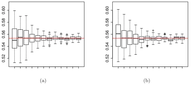
Fig 1. Effect ofk∈ {30,100,1,000,2,000, . . . ,10,000}forε= 0.05. The continuous red line
represents the true MLE value.
0.52
0.54
0.56
0.58
0.60
0.52
0.54
0.56
0.58
0.60
(a) (b)
Fig 2. Effect of ε ∈ {1,0.9, . . . ,0.1,0.05,0.01} for k = 10,000: (a) D = (0.45,0.65); (b)
D= (0,1). The continuous red line represents the true MLE value
and the Euclidean metric we simulate an ABC sample of size 10,000 which, together with Gaussian kernel estimation of the posterior, gives the AMLE ˜
θ= 0.552.
[image:15.612.129.429.121.271.2] [image:15.612.126.433.326.465.2]−0.02
−0.01
0.00
0.01
0.02
µ
0.98
0.99
1.00
1.01
1.02
σ
(a) (b)
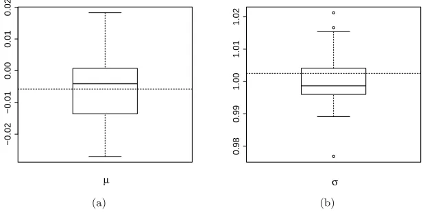
Fig 3. Monte Carlo variability of the AMLE: (a)µ; (b)σ. The dashed lines represent the
true MLE value.
fixed kand two different choices of D. In this case we can note that the effect of ε on the precision is significant. The estimation precision is similar when ε is small for both choices of D. However, we can see that larger values of ε produce the acceptance of more extreme values of θ when combined with the choiceD= (0,1). This is reflected, for instance, in the median of the boxplots corresponding toε= 1 in Figure 2. This interaction arises becauseεis similar in scale to the diameter ofDand would not be expected to produce a noticeable effect in realistic settings in whichD would typically be much larger than ε— smoothing on a similar scale to the total prior uncertainty in the range of the parameters is unlikely to be desirable.
4.2. Normal model
Consider a sample of size 100 simulated from a Normal(0,1) with sample mean ¯
x = −0.005 and sample variance s2 = 1.004. Suppose that both parameters (µ, σ) are unknown. The MLE of (µ, σ) is simply (µ,b bσ) = (−0.005,1.002).
Consider the priors µ ∼ Unif(−0.25,0.25) and σ ∼ Unif(0.75,1.25) (crude estimates of location and scale can often be obtained from data, justifying such a choice; using broader prior support here increases computational cost but does not prevent good estimation), a tolerance ε = 0.01, a sufficient statistic η(x) = (¯x, s), the Euclidean metric, an ABC sample of size 5,000, and Gaussian kernel estimation of the posterior. Figure3illustrates Monte Carlo variability of the AMLE of (µ, σ). Boxplots were obtained using 50 replicates of the algorithm.
4.3. α-stable logarithmic daily returns model
[image:16.612.177.487.121.276.2]−0.10 −0.05 0.00 0.05 0.10
0
50
100
150
200
250
300
350
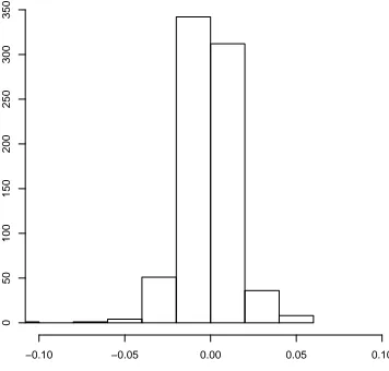
Fig 4. Logarithmic daily returns using the closing price of IBM ordinary stock Jan. 1 2009
to Jan. 1 2012.
using an infinitely divisible distribution. It has been found empirically that these observations have tails heavier than those of the normal distribution, and therefore an attractive option is the use of the 4−parameter (α, β, µ, σ)α−stable family of distributions, which can account for this behaviour. It is well known that maximum likelihood estimation for this family of distributions is difficult. Various numerical approximations of the MLE have been proposed (see e.g. Nolan,2001). From a Bayesian perspective, Peters et al. (2010) proposed the use of ABC methods to obtain an approximate posterior sample of the parameters. They propose six summary statistics that can be used for this purpose.
Here, we analyse the logarithmic daily returns using the closing price of IBM ordinary stock from January 1 2009 to January 1 2012. Figure 4 shows the corresponding histogram. For this data set, the MLE obtained using the nu-merical method implemented in the R package ‘fBasics’ (Wuertz et al., 2010) is (ˆα,β,ˆ µ,ˆ σ)= (1.6295,ˆ −0.05829,−0.0008,0.0078).
Given the symmetry observed and in the spirit of parsimony, we consider the skewness parameterβto be 0 in order to calculate the AMLE of the parameters (α, µ, σ). Based on the interpretation of these parameters (shape, location and scale) and the data we use the priors
α∼U(1,2), µ∼U(−0.1,0.1), σ∼U(0.0035,0.0125)
which due to the scale of the data may appear concentrated but are, in fact, rather uninformative, allowing a location parameter essentially anywhere within the convex hull of the data, scale motivated by similar considerations and any value of the shape parameter consistent with the problem at hand.
[image:17.612.187.365.124.294.2]func-0.5 0.4 0.3 0.2 0.125
1.3
1.4
1.5
1.6
1.7
ε
0.5 0.4 0.3 0.2 0.125
−0.004
−0.002
0.000
0.002
ε
0.5 0.4 0.3 0.2 0.125
0.006
0.007
0.008
0.009
ε
(a) (b) (c)
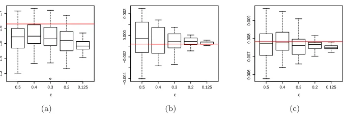
Fig 5. Monte Carlo variability of the AMLE: (a)α; (b)µ; (c)σ. Horizontal lines represent
MLE estimator produced by the R package ‘fBasics’.
tion evaluated on an appropriate grid. We use the grid t ∈ {-250, -200, -100, -50, -10, 10, 50, 100, 200, 250}, an ABC sample of size 2,500, a tolerance ε ∈ {0.5,0.4,0.3,0.2,0.125}and Gaussian kernel density estimation. Figure 5 illustrates Monte Carlo variability of the AMLE of (α, µ, σ). Boxplots were ob-tained using 50 replicates of the AMLE procedure. In general, considerable care must of course be taken in the selection of statistics.
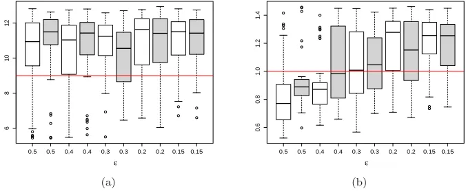
4.4. Superposed gamma point processes
The modelling of an unknown number of superposed gamma point processes pro-vides another scenario with intractable likelihoods which is currently attracting some attention (Cox and Kartsonaki,2012; Mengersen et al.,2013). Intractabil-ity of the likelihood in this case is a consequence of the dependency between the observations, which complicates the construction of their joint distribution. Superposed point processes have applications in a variety of areas, for instance Cox and Smith (1954) present an application of this kind of processes in the context of neurophysiology. In this example we consider a simulated sample of size 88 ofN = 2 superposed point processes with inter-arrival times identically distributed as a gamma random variable with shape parameterα= 9 and rate parameterβ = 1 observed in the interval (0, t0), with t0 = 420. This choice is inspired by the simulated example presented in Cox and Kartsonaki (2012).
[image:18.612.164.502.124.237.2]0.5 0.5 0.4 0.4 0.3 0.3 0.2 0.2 0.15 0.15
6
8
10
12
14
ε
0.5 0.5 0.4 0.4 0.3 0.3 0.2 0.2 0.15 0.15
0.4
0.6
0.8
1.0
1.2
1.4
ε
(a) (b)
Fig 6. Effect ofε∈ {0.5,0.4,0.3,0.2,0.15}fork= 5,000: (a)α; (b)β. The AMLE samples
with 8and9 summary statistics are presented in white and gray boxplots, respectively. The continuous red line represents the true value of the parameter.
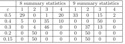
Table 1
Replicate study with a single data realisation. Empirical distribution ofNb for different values ofε
8 summary statistics 9 summary statistics
ε 1 2 3 4 1 2 3 4
0.5 29 0 1 20 33 0 15 2
0.4 5 0 35 10 0 0 50 0
0.3 0 4 46 0 0 37 13 0
0.2 0 50 0 0 0 50 0 0
0.15 0 50 0 0 0 50 0 0
successive points are likely to be useful whenN is small, therefore we consider a second set of summary statistics by adding a ninth quantity based on the third moment: the sample skewness of the intervals between successive points
Pn
j=1(xj−x)¯ 3/(Pnj=1(xj−x)¯ 2/n)3/2. The summary statistics of the simulated
data are (0.210,0.669,−0.355,4.74,0.910,0.476,0.268,0.200,0.493).
[image:19.612.177.385.346.419.2]7.5 8.0 8.5 9.0 9.5 10.0 10.5 11.0
0.8
0.9
1.0
1.1
α
β
7.5 8.0 8.5 9.0 9.5
0.75
0.80
0.85
0.90
0.95
1.00
α
β
(a) (b)
Fig 7. AMLE estimators of β vs. AMLE estimators ofα: (a) 8 summary statistics; (b) 9
summary statistics.
0.5 0.5 0.4 0.4 0.3 0.3 0.2 0.2 0.15 0.15
6
8
10
12
ε
0.5 0.5 0.4 0.4 0.3 0.3 0.2 0.2 0.15 0.15
0.6
0.8
1.0
1.2
1.4
ε
(a) (b)
Fig 8. Effect ofε∈ {0.5,0.4,0.3,0.2,0.15} fork= 5,000: (a)α; (b)β. The AMLE samples
with8 and9 summary statistics are presented in white and gray boxplots, respectively. The continuous red line represents the true value of the parameter.
scatter plots of the AMLE estimators ofβ andαforε= 0.15 and both sets of summary statistics. This scatterplot demonstrates that the mean (α/β) of the gamma distribution is much more tightly constrained by the data than the shape parameter, leading to a nearly-flat ridge in the likelihood surface. The variability in the estimated value of α/β is, in fact, rather small; while the variability in estimation of the shape parameter reflects the lack of information about this quantity in the data and the consequent flatness of the likelihood surface.
[image:20.612.166.516.93.269.2] [image:20.612.173.511.314.453.2]Table 2
Replicate study with 50 data realisations. Empirical distribution ofNb for different values ofε
8 summary statistics 9 summary statistics
ε 1 2 3 4 1 2 3 4
0.5 7 0 24 19 5 0 43 2
0.4 8 0 41 1 3 0 24 23
0.3 1 27 22 0 0 43 7 0
0.2 0 46 4 0 0 44 6 0
0.15 0 47 3 0 0 46 4 0
ABC samples of size 5,000. We can observe that the behaviour of the estima-tors of (α, β) is fairly similar for both sets of summary statistics. Table1 also suggests an improvement in the estimation ofN produced by the inclusion of the sample skewness.
5. Discussion
This paper presents a simple algorithm for conducting maximum likelihood estimation via simulation in settings in which the likelihood cannot (readily) be evaluated and provides theoretical and empirical support for that algorithm. This adds another tool to the “approximate computation” toolbox. This allows the (approximate) use of the MLE in most settings in which ABC is possible: desirable both in itself and because it is unsatisfactory for the approach to inference to be dictated by computational considerations. Furthermore, even in settings in which one wishes to adopt a Bayesian approach to inference it may be interesting to obtain also a likelihood-based estimate as agreement or disagreement between the approaches can itself be informative. Naturally, both ABC and AMLE being based upon the same approximation, the difficulties and limitations of ABC are largely inherited by AMLE. Selection of statistics in the case in which sufficient statistics are not available remains a critical question. There has been considerable work on this topic in recent years (see e.g. Fearnhead and Prangle,2012).
Acknowledgements
We thank two reviewers and an Associate Editor for helpful comments.
References
Abraham, C., Biau, G. and Cadre, B. (2003). Simple estimation of the mode of a multivariate density. The Canadian Journal of Statistics 31: 23– 34.MR1985502
Beaumont, M. A., Zhang, W. and Balding, D. J. (2002). Approximate
Bayesian computation in population genetics.Genetics 162: 2025–2035. Besag, J. (1975). Statistical Analysis of Non-Lattice Data. The Statistician
24:179–195.
Biau, G., C´erou, F. and Guyader, A.(2012). New Insights into Approxi-mate Bayesian Computation. ArXiv preprintarXiv:1207.6461.
Bickel, D. R. and Fr¨uwirth, R. (2006). On a fast, robust estimator of the mode: Comparisons to other robust estimators with applications. Computa-tional Statistics & Data Analysis 50: 3500–3530.MR2236862
Blum, M. G. B.(2010). Approximate Bayesian computation: a nonparametric perspective.Journal of the American Statistical Association 105: 1178–1187. MR2752613
Bret´o, C., Daihi, H., Ionides, E. L. and King, A. A. (2009). Time se-ries analysis via mechanistic models.Annals of Applied Statistics 3: 319–348. MR2668710
Cox, D. R. and Kartsonaki, C.(2012). The fitting of complex parametric models.Biometrika 99: 741–747.MR2966782
Cox, D. R. and Reid, N.(2004). A note on pseudolikelihood constructed from marginal densities.Biometrika 91: 729–737.MR2090633
Cox, D. R. and Smith, W. L. (1954). On the superposition of renewal pro-cesses.Biometrika 41: 91–9.MR0062995
Cule, M. L., Samworth, R. J. and Stewart, M. I.(2010). Maximum like-lihood estimation of a multi-dimensional log-concave density.Journal Royal Statistical Society B 72: 545–600.MR2758237
Dean, T. A., Singh, S. S., Jasra A. and Peters G. W.(2011). Parame-ter estimation for hidden Markov models with intractable likelihoods. ArXiv preprintarXiv:1103.5399v1.
de Valpine, P.(2004). Monte Carlo state space likelihoods by weighted poste-rior kernel density estimation.Journal of the American Statistical Association
99: 523–536.MR2062837
Didelot, X., Everitt, R. G., Johansen, A. M. and Lawson, D. J.(2011). Likelihood-free estimation of model evidence. Bayesian Analysis 6: 49–76. MR2781808
Diggle, P. J. and Gratton, R. J. (1984) Monte Carlo Methods of Infer-ence for Implicit Statistical Models. Journal of the Royal Statistical Society
Duong, T. and Hazleton, M. L.(2005). Cross-validation bandwidth matri-ces for multivariate kernel density estimation.Scandinavian Journal of Statis-tics 32:485–506.MR2204631
Duong, T. (2011). ks: Kernel smoothing. R package version 1.8.5. http:// CRAN.R-project.org/package=ks
Ehrlich, E., Jasra, A. and Kantas, N. (2012). Static parameter esti-mation for ABC approxiesti-mations of hidden Markov models. ArXiv preprint arXiv:1210.4683.
Fan, Y., Nott, D. J. and Sisson, S. A.(2012). Approximate Bayesian Com-putation via Regression Density Estimation.Stat 2: 34–48.
Fearnhead, P. and Prangle, D. (2012). Constructing Summary Statistics for Approximate Bayesian Computation: Semi-automatic ABC (with discus-sion).Journal of the Royal Statistical Society B 74: 419–474.MR2925370
Fukunaga, K. and Hostetler, L. D. (1975). The Estimation of the Gradi-ent of a Density Function, with Applications in Pattern Recognition. IEEE Transactions on Information Theory 21: 32–40.MR0388638
Gaetan, C. and Yao, J. F.(2003). A multiple-imputation Metropolis version of the EM algorithm.Biometrika 90: 643–654.MR2006841
Gouri´eroux, C., Monfort, A. and Renault, E.(1993). Indirect Inference.
Journal of Applied Econometrics 8:S85–S118.
Ionides, E. L.(2005). Maximum Smoothed Likelihood Estimation. Statistica Sinica 15: 1003–1014.MR2234410
Jaki, T. and West, R. W.(2008). Maximum Kernel Likelihood Estimation.
Journal of Computational and Graphical Statistics 17: 976.MR2649075
Jasra, A., Kantas, N. and Ehrlich, E.(2013). Approximate Inference for Observation Driven Time Series Models with Intractable Likelihoods. ArXiv PreprintarXiv:1303.7318.
Jing, J., Koch, I. and Naito, K. (2012). Polynomial Histograms for Multi-variate Density and Mode Estimation.Scandinavian Journal of Statistics 39: 75–96.MR2896792
Johansen, A. M., Doucet, A., and Davy, M.(2008). Particle methods for maximum likelihood parameter estimation in latent variable models.Statistics and Computing 18: 47–57.MR2416438
Konakov, V. D. (1973). On asymptotic normality of the sample mode of multivariate distributions.Theory of Probability and its Applications18: 836–
842.MR0336874
Lehmann, E. and Casella, G.(1998).Theory of Point Estimation (revised edition). Springer-Verlag, New York. MR1639875
Lele, S. R., Dennis, B. and Lutscher, F. (2007). Data cloning: easy max-imum likelihood estimation for complex ecological models using Bayesian Markov chain Monte Carlo methods. Ecology Letters 10: 551–563.
Marin, J.-M., Pudlo, P., Robert, C. P. and Ryder, R.(2011). Approxi-mate Bayesian Computational methods. Statistics and Computing 21: 289–
291.MR2992292
Marjoram, P., Molitor, J., Plagnol, V. and Tavar´e, S.(2003). Markov chain Monte Carlo without likelihoods.Proceedings of the National Academy of Sciences of the United States of America: 15324–15328.
Mengersen, K. L., Pudlo, P. and Robert, C. P.(2013). Bayesian com-putation via empirical likelihood. Proceedings of the National Academy of Sciences of the United States of America 110: 1321–1326.
Nolan, J. P.(2001). Maximum likelihood estimation and diagnostics for stable distributions. In: O.E. Barndorff-Nielsen, T. Mikosh, and S. Resnick, Eds., L´evy Processes, Birkhauser, Boston, 379–400.MR1833706
Parzen, E.(1962). On estimation of a probability density function and mode.
Annals of Mathematical Statistics 33: 1065–1076.MR0143282
Peters, G. W., Sisson, S. A. and Fan, Y.(2010). Likelihood-free Bayesian inference forα−stable models.Computational Statistics & Data Analysis 56: 3743–3756.MR2943924
Pritchard, J. K., Seielstad, M. T., Perez-Lezaun, A., and Feldman, M. T.(1999). Population Growth of Human Y Chromosomes: A Study of Y Chromosome Microsatellites.Molecular Biology and Evolution16: 1791–1798. Robert, C. P., Cornuet, J., Marin, J. and Pillai, N. S. (2011). Lack of confidence in ABC model choice.Proceedings of the National Academy of Sciences of the United States of America 108: 15112–15117.
Romano, J. P.(1988). On weak convergence and optimality of kernel density estimates of the mode.The Annals of Statistics 16: 629–647.MR0947566
Rubio, F. J. and Johansen, A. M.(March, 2012). On Maximum Intractable Likelihood Estimation. University of Warwick, Dept. of Statistics. CRiSM working paper 12–04.
Rudin, W. (1976).Principles of Mathematical Analysis. New York: McGraw-Hill.MR0385023
Sisson, S. A., Fan, Y. and Tanaka, M. M.(2007). Sequential Monte Carlo without likelihoods. Proceedings of the National Academy of Sciences of the United States of America, 104: 1760–1765.MR2301870
Sk¨old, M. and Roberts, G. O. (2003). Density estimation for the
Metropolis–Hastings algorithm. Scandinavian Journal of Statistics 30: 699–
718.MR2155478
Toni, T., Welch, D., Strelkowa, N., Ipsen, A. and Stumpf, M. P. H. (2009). Approximate Bayesian computation scheme for parameter infer-ence and model selection in dynamical systems.Journal of the Royal Society Interface 6: 187–202.
Whitney, K. N. (1991). Uniform Convergence in probability and stochastic equicontinuity.Econometrica 59: 1161–1167.MR1113551
Wilkinson, R. D. (2008). Approximate Bayesian computation (ABC)
gives exact results under the assumption of model error. ArXiv preprint arXiv:0811.3355.