Development of solid state NMR on disordered systems, from bioactive glasses to mullites

(1)

University of Warwick institutional repository: http://go.warwick.ac.uk/wrap

A Thesis Submitted for the Degree of PhD at the University of Warwick

http://go.warwick.ac.uk/wrap/66689

This thesis is made available online and is protected by original copyright.

Please scroll down to view the document itself.

(2)

Development of Solid State NMR on Disordered

Systems, from Bioactive glasses to Mullites

by

Scott Paul King

Thesis

Submitted to the University of Warwick

for the degree of

Doctor of Philosophy

Department of Physics

(3)

List of Tables

3.1 Phase cycling table for simple pulse sequence. . . 53

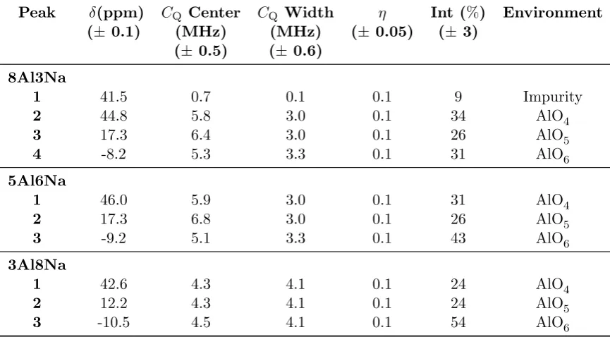
4.1 Compositions of glasses under investigation, with varying Al and Na content. . . 81 4.2 27Al MAS-NMR parameters from simulation of Al doped bioactive glasses

single pulse NMR spectra. . . 84

5.1 Compositions of glasses under investigation, with varying Ga and Na content. . . 99 5.2 Fitting parameters from31P NMR of Ga glass samples. . . 104 5.3 23Na MAS NMR parameters from simulation of Ga doped bio-active

glasses single pulse NMR spectra. . . 111 5.4 71Ga MAS NMR parameters from simulation of Ga doped bio-active

glasses single pulse NMR spectra. . . 115 5.5 17O NMR parameters from simulation of slices from 3QMAS NMR spectra.121

6.1 Compositions of mullite samples under investigation. . . 132 6.2 27_{Al MAS NMR parameters from simulation of mullite single pulse NMR}

spectra. . . 136 6.3 11B MAS NMR parameters obtained from simulating single pulse mullite

NMR data. . . 141 6.4 Simulation parameters from29Si MAS NMR of mullite samples. . . 143

(8)

A.2 23_{Na MAS NMR parameters from simulation of Al doped bioactive}

glasses single pulse NMR spectra. . . 174 A.3 Fitting parameters from31P NMR of Al glass samples. . . 175 A.4 Fitting Results from Time-Domain spin echo fits of 31P REINE curves

forQ1−Q1 and Q1−Q2 peaks for aluminium phosphate glass. . . 176 A.5 Fitting Results from Time-Domain spin echo fits of 31P REINE curves

forQ2−Q2 peaks for aluminium phosphate glass. . . 177 A.6 Fitting Results from Time-Domain spin echo fits of 31P REINE curves

(9)

List of Figures

2.1 Zeeman effect . . . 13

2.2 Euler angles . . . 24

2.3 Frame rotations . . . 26

2.4 Chemical shift anisotropy (CSA) powder patterns . . . 31

2.5 Orientation of the internuclear vector and Pake Doublet . . . 32

2.6 Energy level diagram for isolated spin I = 1₂ nucleus and for a pair of coupled spinI = 1₂ nuclei, in the presence of a magnetic field . . . 36

2.7 Energy level diagram for a spin 3₂ nucleus. . . 41

2.8 Typical second order quadrupole broadened lineshapes under MAS. . . . 45

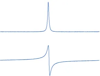
3.1 Absorptive and dispersive lineshapes . . . 48

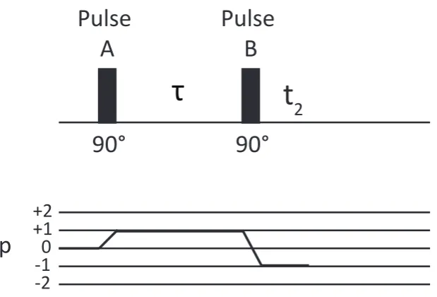
3.2 Simple pulse sequence . . . 51

3.3 Spin echo pulse sequence . . . 56

3.4 INADEQUATE, refocused INADEQUATE and REINE pulse sequence. 60 3.5 J-HMQC pulse sequence . . . 67

3.6 MQMAS pulse sequence . . . 70

3.7 Splitt1 MQMAS pulse sequence . . . 71

3.8 Change in Quadfit lineshape upon change in theCQ width . . . 76

4.1 27Al single pulse MAS-NMR spectra and simulated fits for each Al glass composition. . . 83

4.2 23Na single pulse MAS-NMR spectra and simulated fits for each Al glass composition. . . 85

4.3 31P single pulse MAS-NMR spectra for each Al glass composition. . . . 86

(10)

4.5 Time-domain spin echo curves obtained from the summed intensity for

theQ1-Q1 and Q1-Q2 31P REINE peaks for each Al glass composition. . 90

4.6 31P Q1-Q2 REINE peak pixel by pixel fitting for Al glasses . . . 92

4.7 Time domain spin echo curves obtained from the summed intensity of the31P Q2-Q2 REINE peaks for Al glasses . . . 94

5.1 31P single pulse MAS NMR spectra and simulated fits for the three Ga glass series. . . 103

5.2 31P REINE spectra atτj = 0.8 ms for each Ga glass composition. . . . 107

5.3 Time-domain spin echo curves obtained from the summed intensity for theQ1-Q2 and Q2-Q2 31P REINE peaks for each Ga glass composition. 108 5.4 31P Q1-Q2 REINE peak pixel by pixel fitting for Ga glass compositions 109 5.5 23Na single pulse NMR spectra and simulated fits for Ga glasses . . . . 112

5.6 71Ga single pulse MAS-NMR along with simulated fits for Ga glasses . . 114

5.7 {31_P_}_-71_Ga _J_{-HMQC of P45Ga15 glass} _{. . . 117}

5.8 17O Spin Echo NMR of P50Gax17O labelled samples . . . 118

5.9 17O 3QMAS NMR of P50Gax 17O labelled samples . . . 119

5.10 Slices of NBO resonance from17_{O 3QMAS of P50Gax glasses. . . 120}

6.1 Diagram of the mullite structure. . . 127

6.2 Diagram of the B doped mullite structure. . . 130

6.3 Multifield single pulse27Al MAS NMR spectra along with simulated fits of 3:2 mullite samples. . . 135

6.4 Multifield single pulse27Al MAS NMR spectra along with simulated fits of sillimanite . . . 137

6.5 Multifield 3QMAS27Al spectra of 3:2 mullite samples. . . 138

6.6 Multifield27_{Al MAS NMR spectra of 2:1 mullite.} _{. . . 140}

6.7 11B single pulse MAS NMR and 3QMAS spectra of B doped mullites. . 140

6.8 29Si single pulse MAS NMR spectra along with simulated fits of 3:2 mullites. . . 142

(11)

(12)

Acknowledgments

Firstly, I would like to thank my supervisor Dr John Hanna, for his guidance and support throughout every aspect of this PhD project. I would also like to thank my second supervisor Professor Steven Brown for his input, particularly early on in my research whilst getting to grips with 2D NMR and the REINE pulse sequence. I’m extremely grateful to the Engineering and Physical Sciences Research Council (EPSRC) for helping to fund my project, without which this research wouldn’t have been possible. I am indebted to the great support of everyone in the Solid State NMR group at the University of Warwick, in particular Dr Andy Howes and Dr Tom Kemp for assisting with any technical issues arising in the lab, Dr Dinu Iuga for his guidance whilst using the 850 MHz facility, and Dr Greg Rees for his assistance in teaching me NMR in the early stages of my project.

The many collaborators I have had the pleasure to work with throughout my time in NMR, from a vast range of institutions, enabled me to obtain experience in a wide range of research areas, which I acknowledge helped me to develop as an NMR spectroscopist. I would like to thank Dr Hanna L¨uhrs and Professor Reinhard Fischer (University of Bremen) for providing me with high quality mullite samples and for their knowledge on the mullite systems, always happy to answer any questions I may have relating to their complex structure. In addition, everyone involved in the collab-orations involving the glass materials; from providing samples, helping with labelling, and informative discussions, including Dr Richard Martin (Aston University), Professor Jonathan Knowles (UCL), Dr Jodie Smith and Dr Dave Pickup (University of Kent). Dr. Paul Guerry is acknowledged for providing the MATLAB fitting routines used in the analysis of the REINE data.

(13)

Declarations

I hereby declare that this thesisDevelopment of Solid State NMR on Disordered Systems, from Bioactive glasses to Mullitesis an original work and has not been submitted for a degree or diploma or other qualification at any other University.

Results from other authors are referenced in the usual manner throughout the text. All collaborative results are indicated in the text along with the nature and extent of my individual contribution, a brief summary is given here:

In Chapter 4 the samples were synthesised by Dr Jodie Smith and Dr Dave Pickup at the University of Kent. The 27Al measurements presented in Chapter 4 have been carried out by myself and feature in the publication “Structural study of Al₂O₃ -Na₂O-CaO-P₂O₅ bioactive glasses as a function of aluminium content”. J.M. Smith, S. P. King , E. R. Barney, J. V. Hanna, R. J. Newport, and D. M. Pickup. The Journal of Chemical Physics, 2013, 138, 034501. The MATLAB package used for analysis of the REINE data was kindly provided by Paul Guerry, which itself had previously been modified from Paul Hodgkinsons fitting routines.

The gallium phosphate glass series in Chapter 5 was synthesised by Professor Jonathan Knowles’ group at UCL, with the exception of the 17O labelled samples which were provided by Dr Richard Martin at Aston University. 17O labelled CaO used for the synthesis of the labelled samples was kindly provided by Franck Fayon (Universite d’Orleans).

(14)

Abstract

Phosphate glasses for potential applications as bioactive materials have been studied using Solid state Nuclear Magnetic Resonance (NMR), owing to the fact that their bioactivity is strongly correlated to their atomic structure. A multinuclear NMR approach has been conducted on numerous series of phosphate bioactive glasses includ-ing 31P, 23Na, along with 27Al MAS NMR on a series of Al doped glasses, and the less widely studied 71Ga and 17O MAS NMR on multiple series of Ga doped glasses. In addition, the first implementation of the recently developed 31P refocused INADE-QUATE Spin-Echo (REINE) experiment on a coherent series of glasses has been shown, providing greater insight into the distribution ofJ couplings throughout the phosphate network.

Upon incorporation of Al into the phosphate network, 27Al MAS NMR has shown a subsequent change from initially octahedral to tetrahedral Al coordination. In addition, an increase in shielding and decrease in the quadrupolar parameterCQof the

Na ions from 23Na MAS NMR, along with a decrease in the 31P J coupling indicated from the REINE data, evidences the role of Al within the glass network cross linking phosphate chains, resulting in a strengthened more condensed network.

In the Ga doped glass series the 71Ga MAS NMR data shows a similar trend for the Ga coordination as found in the Al series, with the23Na MAS NMR also indicating comparable results. The31P REINE results however, do not provide observable trends, thus indicating that the Ga is having a slight different influence in the glass network to that of the Al cation. 17O 3QMAS results show the presence of both non bridging and bridging oxygens as expected in these systems.

Mullite materials are of interest to material scientists owing to their favourable properties, making them ideal for ‘advanced ceramic’ applications. However, the struc-ture of mullite is complex owing to the disorder, arising from the vacancies present in the aluminosilicate network. A comprehensive multinuclear solid state MAS NMR investigation has been carried out on the structure of both undoped 3:2 mullite, and B doped 3:2 mullite materials. 27Al single pulse MAS NMR has enabled the identification of the octahedral and tetrahedral sites present, along with the 27_{Al 3QMAS experiment}

providing conclusive evidence of the Al tri-cluster sites in the structure. 100 % 29Si labelled samples have enabled the acquisition of quantitative and high resolution 29Si MAS NMR data, along with 29_{Si refocused INADEQUATE and}_{29_Si_}_-27_Al _J_-HMQC

correlation experiments, providing detailed information on the connectivities in the aluminosilicate network. Both the 27Al and 29Si MAS NMR data have enabled deter-mination of the nature of the tri-cluster site. 11_{B MAS NMR on B doped 3:2 mullite}

(15)

Abbreviations

3Q Triple Quantum

ADP Ammonium Dihydrogen Phosphate AlT* Aluminium site within a tri-cluster BO Bridging Oxygens

COSY Correlation Spectroscopy CP Cross Polarisation

CRAMPS Combined Rotation and Multiple-Pulse Sequence CSA Chemical Shift Anisotropy

CT Central Transition CW Continuous Wave

DAS Dynamic Angle Spinning DFT Density Functional Theory DLS Distance Least Squares DNP Dynamic Nuclear Polarisation DOR Double Angle Rotation

DQ Double Quantum

EFG Electric Field Gradient

EPR Electron Paramagnetic Resonance FDA Food and Drug Administration (US) FID Free Induction Decay

FTIR Fourier Transform Infrared Spectroscopy

HMQC Hetronuclear Multiple Quantum Correlation Experiment

Hz Hertz

INADEQUATE Incredible Natural Abundance Double Quantum Transfer Experi-ment

(16)

LAB Lab Reference Frame MAS Magic Angle Spinning

MQMAS Multiple Quantum Magic Angle Spinning Experiment MRI Magnetic Resonance Imaging

NBO Non Bridging Oxygens NMR Nuclear Magnetic Resonance PAS Principle Axis Rotation Frame REINE Refocused INADEQUATE Spin-Echo rf Radiofrequency

S/N Signal to Noise Ratio SQ Single Quantum TMS Tetramethylsilane TO Terminal Oxygens

TPPI Time-Proportional Phase Incrementation TQ Triple Quantum

XRD X-Ray Diffraction

YAG Yttrium Aluminium Garnet

(17)

Chapter 1

Introduction

1.1 History of NMR

Before the 20th century the subject of nuclear physics had not really been established, with the discovery by Rutherford in 1907 of the model of the atom consisting of a dense positive nucleus surrounded by the negative electron, and later in 1932 the nucleus by James Chadwick, both laying down the groundwork for the field.[1, 2] It was only a short time after this discovery of the neutron in 1938, that the resonance effect of nuclear matter was observed by Isidor Isaac Rabi. Rabi’s experiment consisted of a molecular beam of LiCl that was deflected by an inhomogeneous magnetic field and subsequently refocused by a second field. Resonance was observed when upon variation of the field a drop in intensity due to a failure in the refocusing occurred.[3] Rabi was awarded the Nobel prize in physics for his work in 1944 “for his resonance method for recording the magnetic properties of atomic nuclei.”

(18)

MIT carried out the first ‘solid state’ NMR experiment, detecting NMR absorption of protons in a tank of paraffin, upon changing the applied magnetic field. Meanwhile, Felix Bloch at Stanford carried out the first ‘liquid state’ NMR, using a transmitter receiver set up in the presence of a magnetic field, to obtain nuclear induction in water. Both Bloch and Purcell were credited with the discovery of what we think of as modern day NMR, with both of their results published early in 1946, for which they were subsequently awarded the Nobel Prize in 1952 “for their development of new methods for nuclear magnetic precision measurements and discoveries in connection

therewith.” [5–7] It is an interesting point that the two different methods implemented by the two groups for detecting resonances actually represent the two methods for explaining the NMR phenomenon, with the absorption from Purcell’s method best described by quantum mechanics, and Bloch’s method of induction described by the classical description of electromagnetic induction.

Early work in the field of NMR was predominantly carried out by Physicists, in the hope of using the nuclear resonance frequency of a nuclear species to measure its magnetic moment, as it was a non destructive way to obtain these precision mea-surements. This work was based on the early assumption that the resonance frequency of a particular nuclear species depended only upon the strength of the applied field. However, this was all about to change during the 1950s with the surprise discovery by Proctor and Yu that the 14N resonance frequency observed depended strongly on the chemical compound under observation.[8] This effect had also been observed by Dickin-son who noted “for 19F the value of the applied magnetic fieldH0 for nuclear magnetic

resonance at a fixed frequency depends on the chemical compound containing the

flu-orine nucleus.”[9] A year earlier Walter Knight had observed a similar phenomenon in a series of metals, however this was due to delocalised conducting electrons in the vicinity of the metal nucleus, what we now know as the ‘Knight Shift’ in metals.[10] A full theory of the chemical shift was presented in 1950 by Ramsey.[11] The discovery of the chemical shift, resulting in different resonance frequencies for a particular nuclear species due to differences in the chemical structure, ultimately led to the technique being taken up by chemists to become the vital tool for structural characterisation it is today.

(19)

looking at a single crystal of gypsum (CaSO₄.2 H₂O), containing two protons which represent the only significantly magnetic species when looking at its 1H resonance.[12] The observed pair of doublets, indicated that each proton could see the two states of its coupled neighbour, both up and down. Pake then expanded this to powdered solids to identify the ‘Pake doublet’, arising from the different orientations of different crystals within a powder. Using NMR to observe H atoms became a useful tool to exploit, due to the difficulty in observing these small nuclei by other techniques, such as XRD, due to scattering effects from heavier atoms. In addition, the ability to probe and measure intermolecular distances due to the 1/r3 _{dependence of the dipolar interaction}

was also noted by Pake. The commonly held view of the turning point towards ‘high resolution’ NMR actually came from the work of Dharmatti and Packard in 1951.[13] Due to improvements in magnet inhomogeneity, they managed to observe a spectrum of ethanol showing three distinct lines with ratios 1:2:3 for the first time, providing direct evidence for the CH₃CH₂OH formula.

(20)

Poor sensitivity from low Boltzmann factors of NMR states at room temperature was a key challenge that was successfully tackled in 1963 by Klein and Barton.[16] They determined that by accumulating many relatively rapid scans of the full spectrum, so that the signals add coherently whereas the noise adds randomly, signal to noise may be enhanced by one to two orders of magnitude without sacrifice of bandwidth. This was then followed in 1966 by Ernst and Anderson by the Fourier transform method, where short pulses of high power rf radiation were applied with the response of the system observed and Fourier transformed to obtain a frequency domain spectrum.[17] This again improved sensitivity and made data acquisition a much faster process. Although at this stage computing power to carry out the Fourier transformations meant that obtaining a fully processed spectrum could take a matter of days.

Magnet design was an early problem to overcome, with permanent and electro-magnets both being used by different research groups, however they were limited by their strength. The first superconducting magnet for NMR studies was implemented in 1964, which meant much higher fields were accessible, although the economy of these early systems was poor with short liquid helium hold times, leading to refills being required twice a week. [18]

With the discovery of the chemical shift and later theJ coupling the dominance of solution NMR became widespread, with narrow resonances obtained emanating from the molecular tumbling in solution removing any anisotropies.[19, 20] A significant breakthrough in solid state NMR came with the observation that interactions causing broadening of resonances had an angular dependence that could be removed upon successful rotation of the sample at a well defined angle. Magic angle spinning (MAS) was invented by two groups simultaneously; E. Raymond Andrew in the UK, and by I.J. Lowe in the US.[21–23] However, its commercially viability wasn’t appreciated until much later on due to the difficulty in the experimental design of a stable MAS method, with solution NMR remaining the more accessible and widely researched area.

(21)

found to be reproducible, he had discovered the spin echo.[25]. This was later modified into the conventional 90◦-τ /2-180◦-τ /2 spin echo by Carr and Purcell, which went on to become the basic building block for a wide range of future NMR pulse sequences.[26] The desire to manipulate spins was generally twofold; to enhance signal due to the poor sensitivity of NMR, or to exploit or remove a particular NMR interac-tion. Cross polarisation (CP) exploited the first of these, transferring polarisation from the more abundant spin to the less abundant spin, whereas heteronuclear decoupling achieved the second by suppressing broadening due to undesired interactions.[27, 28] Pines and his co-workers combined the two techniques to obtain a 13_{C chemical shift}

spectrum of a solid using this dilute nuclei.[29] The idea to combine the approach of CP with heteronuclear decoupling whilst also under magic angle spinning of Stejskal and Schaefer successfully achieved removal of broadening due to anisotropic interactions, with the larger homogeneous dipolar broadening removed by decoupling due to it being too large to be successfully averaged away by achievable MAS rates at the time, and with the smaller chemical shift anisotropy (CSA) removed by MAS.[30]

The idea for 2D NMR spectroscopy was first proposed by Jean Jeener at the Ampere International Summer School II, (Basko Polje, 1971), but the basic theory and first experiments were published by Richard R. Ernst’s group.[31] This seminal paper laid the groundwork for many 2D experiments to come, including the 2D heteronu-clear correlation,[32, 33] the 2D INEPT (Insensitive Nuclei Enhanced by Polarisation Transfer),[34] the combined rotation at the magic angle and multiple pulse (CRAMPS) technique,[35] and the homonuclear INADEQUATE, [36] contributing to the wealth of information achievable from manipulating spins via NMR.

Arguably one of the most significant discoveries in the field of magnetic reso-nance, or at least the one most recognisable to the general public, would be in its use to form images, particularly of human organs for medical diagnostics. The first Magnetic Resonance Imaging (MRI) images were collected in 1974 by Peter Mansfield in the UK and Paul C. Lauterbur in the USA, where they used magnetic field gradients for the spatial localisation of NMR signals.[37, 38] This achievement granted them the joint award of the Nobel Prize in Physiology or Medicine in 2003, after the technique had already progressed into a huge field of research in its own right.

(22)

Nuclear Polarisation (DNP), with the aim of enhancing weak signals obtained in NMR. DNP was first proposed by Overhauser in 1953 as a means of enhancing nuclear polar-isation via transferring polarpolar-isation from the electrons of paramagnetic impurities by microwave irradiation close to the electron resonance frequency, enhancing the signal obtained.[39] Early studies showed its effect in enhancing signals in metals, then sub-sequently liquids.[40, 41] Since the early 90s however, with improvements of microwave sources, DNP has undergone a new ‘renaissance’, with papers by Griffin and co-workers showing high field MAS-DNP using a gyrotron source.[42, 43] This was followed by the invention of the dissolution DNP method, where a factor of 10,000 enhancement for liquid signals was achieved. Whereby in this method the sample is polarised at low temperature by microwave irradiation, the sample is then dissolved in a hot solvent and quickly put into the NMR tube in the magnetic field where detection occurs.[44]

During the early days of NMR, quadrupole nuclei were difficult to study, ow-ing to them experiencow-ing large broadenow-ing from the quadrupole interaction at the low magnetic fields available at the time. However, research to combat these effects was not neglected, with line narrowing methods developed, with initial studies using con-ventional MAS, leading to the more technically advanced methods of DOR and DAS to remove the residual second order quadruple effects.[45–50] However the real turning point for studies of quadrupole nuclei came in 1995 with the ground breaking pulse sequence by Frydman and Harwood, the multiple-quantum magic-angle spinning (MQ-MAS), successfully tacking the problem of broadening from the 2nd order quadrupole interaction which isn’t removed by conventional MAS.[51] The MQMAS experiment is still a routinely used tool for solid state NMR spectroscopists, with its implementation widely shown throughout this thesis.

(23)

1.2 NMR of Bioactive Phosphate Glasses: Motivation

An area of particular interest for solid state NMR spectroscopists has been in the study of disordered materials, due to the specify granted by the NMR technique. Other methods of structural characterisation, such as X-ray diffraction, rely upon long range periodicity, restricting their use on disordered materials which lack this long range order. Glass is such a material, with great technological importance, possessing order only on the more local nuclear scale with no long range periodicity.

Early solid state NMR studies on glasses first appeared in the 1950s,[54] al-though due to the broad nature of the NMR resonances arising from the vast array of nuclear sites found within its disordered structure, solid state NMR on glass sys-tems did not really catch on until the use of magic angle spinning could be used in pulsed Fourier transform NMR studies, to achieve suitable line narrowing.[55–58] A lot of early MAS studies focused on silicate based glasses, permitting determination of the silicon coordinations present within the network. Phosphate based glasses however, were not neglected, with early work by Brow,[59, 60] and comprehensive reviews of early NMR phosphate glass results given by Eckert and Kirpatrick and Brow,[61, 62] proving NMR to be a big contributor in the field, due to the vast array of structural in-formation obtained along with its non destructive nature, whilst requiring little sample preparation. Despite the disordered nature of these structures, from amassing the vast array of data from the numerous studies, simple structural models have been created, with the publications by Hoppe in 1996, and Brow at the turn of the 21st century, showing the significant progress in the understanding of these disordered phosphate materials.[63, 64]

(24)

form a Hydroxyapatite layer in vivo that would not get rejected by the body, due to a major proportion of bone being composed of Hydroxyapatite. Thus BioglassR _was

developed, a glass comprising of Ca and phosphate, within a Na₂O -SiO₂ matrix.[65] The first implementation of BioglassR _{clinically was in 1985 to solve hearing loss, by}

replacing bones within the inner ear with a BioglassR _{substitute. A review of the}

mo-tivation behind the discovery of BioglassR _{and its history through the past 40 years is}

given in full by Hench in “The Story of BioglassR_”.[66]

Technological advances in silicate based BioglassesR _{have not been the only area}

of successful research in the field of biomaterials, with Ca phosphate based bioceramics used in dentistry and medicine for over 20 years.[67] Attention has also been focused on developing phosphate based bioactive glasses, similar to the original BioglassR_{. The}

advantage of a glass material is that a wide variety of dopant cations can be incorpo-rated to the structure, with the purpose of fulfilling a specific role. In comparison to the silicate based bioactive glasses, which have break down times within the body on the order of years,[68] phosphate bioactive glasses have much faster dissolution rates which could allow them to perform different functions. For instance, phosphate bioac-tive glasses have been developed as novel delivery devices providing controlled release of ions such as antibacterial Ag or Cu.[69, 70] In addition, various developments for phosphate glasses for hard tissue engineering as biodegradable scaffolds that are even-tually replaced by natural tissue has been proposed, with a comprehensive review of the area given by Abou Neel and Pickup. [71]

The key characteristics of phosphate bioactive glasses is both the bioactivity and the dissolution rates, as control of both can allow specific functions to be achieved, with numerous studies focused on measuring both of these factors for particular glass compositions.[72–77] Both bioactivity and dissolution rates are strongly correlated to the atomic structure of the glass network, thus a detailed understanding of the struc-ture, permits the greatest control of the glasses properties. In recent years, many NMR studies on phosphate bioactive glasses have been undertaken, with the technique shown to provide detailed valuable structural information.[71, 78, 79]

(25)

NMR will be used, including the implementation of the 31_{P REINE pulse sequence on}

a series of glasses for the first time, providing valuable information on the disorder in the phosphate network. 17O and 71Ga NMR will also be presented, which previously have proved difficult to study using solid state MAS NMR, due to their quadrupole nature and their low natural abundance (in particular 17O, which is only 0.037 %). The intention is to provide a much deeper insight into the structure of these disordered systems, with the ultimate aim of helping to further stimulate their use as potential biomaterials.

1.3 NMR of Mullite Structures: Motivation

Understanding and studying the structure of ceramic materials is important not only owing to their occurrence in nature, but also due to their widespread production and use for over thousands of years for wide ranging applications. The aluminosilicate ce-ramic mullite is no exception to this, taking its name from the Isle of Mull in Scotland where it was initially discovered, in regions where hot lava comes into contact with Al₂O₃ rich sedimentary rocks.[80] Despite its rare presence in nature, mullite is a com-mon phase in many conventional man made ceramics including clay products, pottery, porcelains, sanitary ceramics, refractories and in structural clay products like building bricks, pipes and tiles. Thus, mullite has arguably had a large influence indirectly on the development of civilisation throughout the history of mankind. Recently mullite has gained significant interest for use in ‘advanced ceramics’ due to its very appeal-ing properties, includappeal-ing high thermal stability, low thermal expansion, low thermal conductivity, high creep resistance, corrosion stability, and its hard wearing nature.[81] The fact that the starting materials required for mullite formation are abundant in large quantities on earth, and the ability of mullite to form a solid solution in a large Al₂O₃/SiO₂ range, giving it the ability to incorporate a wide range of foreign cations, coupled with the fact that the structural principles of mullites can be extended to a wide ‘family range’ of related phases with different compositions, all add to its appeal for engineers and materials scientists alike.

(26)

instead of the 1:1 (Al₂O₃SiO₂) composition as was commonly thought prior to this.[82] The general formula for the structure of mullite is Al2[Al2+2xSi2−2x]O10−x withx

typ-ically varying from x = 0.2 to 0.9. Many studies on the crystallographic structure of mullite have since been published, with the general consensus being that its structure is very similar to that of the crystalline aluminosilicate sillimanite (Al₂SiO₅).[80, 83, 84] Like sillimanite, mullite consists of chains of Al octahedra running down the crystallo-graphicc-axis, with these chains cross linked by tetrahedral double chains of (Al,Si)O4

tetrahedra. In mullite however, some of the O bridging the tetrahedra are vacant (thus making it distinct from sillimanite), resulting in the formation of proposed tri-cluster sites (T₃O). This leads to a slight disorder in the structure due to this vacancy, mak-ing the creation of an absolute model of the mullite structure incomplete, due to the complexity of the vast array of possible crystallographic sites present.

As already mentioned, one of the favourable properties of mullites lies in its ability to incorporate a wide range of different cations, whilst still retaining the mullite type structure and thus its favourable properties. Al borates are a related class of material that like mullites possess stability to very high temperatures and pressures. The Al₁₈B₄O₃₃ phase (9 Al₂O₃.2 B₂O₃) has gained specific interest, used as both a refractory lining due to its low thermal expansion and its corrosion resistance against B rich glasses, and for the reinforcement of metal matrices.[85, 86] There are many phases within the Al₂O₃-B₂O₃ series which are structurally related to mullite, and therefore a combination of the two systems promises a great potential to design high-performance materials. A solid solution between mullite and Al₁₈B₄O₃₃ was proposed in the 1950’s with the term ‘B mullite’ or ‘boron-mullite’ introduced by Werding and Schreyer.[87, 88] Recent work has however shown that there is no complete solid solution between mullites and Al borates.[86, 89, 90] Although, significant changes of lattice parameters bandcoccurs with B doping, in contrast no significant changes are observed for lattice parameter a, which is linearly correlated with the Al/Si ratio in mullite.[86, 89, 90]

(27)

of the tri-cluster species.[92] Further 29_{Si assignments have been carried out in many}

studies since, most notably by Ban and Okada, Jaymeset al., and Schmuckeret al..[93– 96] However the most conclusive evidence of the tri-cluster species has been presented by Bodart et al. from 27Al 3QMAS measurements on a 2:1 mullite system.[97] The suitability of using solid state MAS NMR to probe the mullite structure emanates from mullite crystallography not being straightforward, due to the vacancies resulting in an apparent disorder. Therefore, NMR remains a key tool in its structural characterisation, due to its nuclear specificity, probing the nuclear sites directly.

(28)

Chapter 2

NMR Theory

The theory in this section is based upon a number of sources, mainly the texts: ‘In-troduction to Solid State NMR Spectroscopy’ M.J. Duer.[98] ‘Spin Dynamics’ M.H. Levitt.[99] ‘NMR: the Toolkit’ P.J Hore, J A. Jones, and S. Wimperis.[100] ‘Multinu-clear Solid State NMR of Inorganic Materials’ K.J.D. MacKenzie, and M.E. Smith.[101] ‘Solid-state NMR : basic principles & practice’ D.C. Apperley, R.K. Harris, and P. Hodgkinson. [102]

2.1 Zeeman Interaction

All subatomic particles have a series of fundamental properties such as mass and charge, however a further intrinsic property determined from Quantum Mechanics is that of spin angular momentum. This is defined by the spin angular momentum quantum number,I, which can take positive integer or half integer values, and for atomic nuclei takes a specific value for each individual isotope, dependent on the constituent nucleons. Further to this, the spin angular momentum is quantized in units of ¯hinto 2I+1 possible energy levels, represented by the azimuthal quantum numberm,m= +I,+I−1, ...,−I. In the absence of a magnetic field all of these energy levels are degenerate. However, in the presence of an external magnetic field this degeneracy is lifted causing the spin states to split, resulting in a separation of energy levels. This is due to the interaction between B0 and the magnetic moment and is commonly known as the

Zeeman Effect, as shown in Figure 2.1.

(29)

m

−

½

½ |α>

|β>

ω

₀

B

=

B

₀

B

= 0

Figure 2.1: Diagram showing the Zeeman effect for a I = 1₂. In the absence of a magnetic field the energy levels are degenerate. Whereas application of a magnetic field, B0, lifts the degeneracy resulting in two energy levels α and β, m = 1₂ and −1₂,

respectively, with an energy difference in frequency units of ω0 between them.

E =−µ·B0 (2.1)

where µis the magnetic moment represented by:

µ=γI, (2.2)

and γ is the gyromagnetic ratio specific for each individual nuclei. However, in NMR we want to express this in terms of Quantum Mechanical operators, so the Zeeman energy Hamiltonian in a static field is represented by:

ˆ

HZ =−µ·B0. (2.3)

By convention when the angular momentum is aligned in the z-direction then, I = (0,0, Iz), as is the external field,B0= (0,0, B0), and using Equation 2.2 the

Hamilto-nian can be written as:

ˆ

HZ=−γIˆzB0 (2.4)

or

ˆ

HZ =ω0Iˆz. (2.5)

(30)

ω0 =−γB0. (2.6)

Therefore, the Larmor frequency is dependent upon the external magnetic field applied, and due to the gyromagnetic ratio being specific for each type of nucleus, it has a different strength depending on the nucleus in question.

A quantum mechanical description is necessary for the most accurate description of an NMR experiment. The state of a quantum mechanical system can be described by a quantum mechanical wavefunction |ψi which represents the physical properties of the system. An operator can be defined that corresponds to an observable quantity, for example energy or angular momentum, that acts upon the wavefunction. Upon repeating an experiment many times the average value we obtain is represented by the expectation value:

D ˆ A E

=hψ|Aˆ|ψi. (2.7)

Application of the relevant angular momentum operator Îx, Îy, Îz, Î2, which represent

the x, y, z components of the nuclear spin and magnitude of the nuclear spin squared respectively, can lead to observables relating to the nuclear spin. This set of operators obey the commutation relations:

[ ˆI2,Iˆz] = 0 (2.8)

[ ˆIx,Iˆy] =iIˆz (2.9)

and any cyclic permutation of the subscripts, and are linked by the relation:

ˆ I2_{= ˆ}_I2

x+ ˆIy2+ ˆIz2. (2.10)

These commutation relations show that as only one component of the spin angular momentum commutes with the total spin angular momentum, only one component is observable at a particular time, by convention ˆIz. In addition the individual components

don’t commute with each other.

(31)

ˆ

Iz written as |I, mi, or:

ˆ

Iz|I, mi=m|I, mi. (2.11)

For a spin I = 1₂ nucleus, which is the simplest case relevant for NMR,m = +1₂ and

−1₂, represented asα= 1₂ andβ =−1₂, spin up and spin down, respectively. Therefore, the eigenvalues become:

ˆ

Iz|αi= +

1 2|αi

ˆ

Iz|βi=−

1

2|βi (2.12)

and from Equation 2.5:

ˆ

H |αi= +1 2ω0|αi

ˆ

H |βi=−1

2ω0|βi. (2.13)

Thus the difference between the Zeeman states is ω0, as stated in Equation 2.5. From

Equation 2.12 we can use the eigenvalues to construct a matrix representation of the ˆ

Iz operator:

ˆ Iz =

  

1

2 0

0 −1 2

 

. (2.14)

The complete wavefunction is a superposition of the α and β basis sets:

|ψi=cα|αi+cβ|βi (2.15)

wherecα and cβ represent the contribution of each state. The expectation value of the

ˆ

Iz operator using Equation 2.7 is given by:

D ˆ Iz

E = 1

2(cαc

∗

α−cβc∗β), (2.16)

showing that the longitudinal component is directly related to the probability of the system been found in either of these spin states.

In contrast, operators with x and y angular momentum don’t have |αi and |βi

(32)

ˆ Ix|αi=

1 2|βi

ˆ Ix|βi=

1 2|αi ˆ

Iy|αi=

1

2i|βi Iˆy|βi= 1 2i|αi.

(2.17)

In matrix form these ˆIx and ˆIy operators are:

ˆ Ix =

  

0 1₂

1 2 0    ˆ Iy =

  

0 −1 2i 1

2i 0

 

 (2.18)

with expectation values given by:

D ˆ Ix

E = 1

2(cαc

∗

β+cβc∗α) (2.19)

D ˆ Iy

E = 1

2i(cαc

∗

β −cβc∗α) (2.20)

2.2 Density Operator

The methods outlined in the previous section are adequate for describing simple sys-tems, however for systems consisting of many spins, or forI >1₂, a linear treatment can become complicated involving many terms. The density operator method is a much more convenient approach utilising matrices. The density operator can be defined as:

ˆ

ρ=|ψi hψ| (2.21)

where the overbar represents an ensemble average of the spin system. The density matrix is:

ρrs=hr|ρˆ|si=crc∗s. (2.22)

For a single spin this density matrix becomes:

ρ=   

cαc∗α cαc∗_β

cβc∗α cβc∗β

 

(33)

therefore, we now have a matrix ρ, that relates to the sample, and one that relates the measurement of a particular operator, ˆA. A product of the two yields:

ρAˆ=   

cαc∗α cαc∗β

cβc∗α cβc∗β

  

  

Aαα Aαβ

Aβα Aββ

 

 (2.24)

=   

cαc∗αAαα+cαc∗_βAβα cαc∗αAαβ+cαc∗_βAββ

cβc∗αAαα+cβc∗_βAβα cβc∗αAαβ+cβc∗_βAββ

 

 (2.25)

and upon inspection of Equation 2.24 above it can be seen that the expectation value of this operator in terms of this density operator is:

D ˆ

AE=T r[ρA]. (2.26)

The above equation shows that independent of the number of spins within the system, any macroscopic observation of the system can be represented by the two operators representing the measured observable and the entire spin ensemble.

If we compare Equation 2.23 to the expressions for the expectation values of ˆ

Iz, Equation 2.16, it can be seen that ˆIz is represented by like terms, therefore the

diagonal elements of Equation 2.23 represent populations of basis functions. Whereas the expectation values for ˆIxand ˆIy, Equations 2.19 and 2.20, show that the off diagonal

elements represent a mixture of states, known as coherences.

2.2.1 Evolution of the Density Operator

A NMR experiment consists of periods of free precession and rf pulses changing over time, which can be described by the time dependent Schr¨odinger equation:

d

dt|ψi=−i ˆ

H |ψi. (2.27)

We can use this to determine how the density operator changes over time:

dρ

(34)

this is known as the Liouville von-Neumann equation and has the solution:[100]

ˆ

ρ(t) =e−iHˆtρˆ(0)e+iHˆt = ˆU(t) ˆρ(0) ˆU(t)−1.

(2.29)

This is an important result as it states that if we know the density operator at a starting point (t = 0), and if we know the Hamiltonians, then we can calculate the density operator at any later time, t. Here ˆU(t) is known as the propagator, which if

ˆ

H is constant, can be expressed as:

ˆ

U(t) =e−iHˆt. (2.30)

IfHˆ is not constant then the propagator can be separated into a series of Hamiltonians each acting consecutively for a time period,e.g.,

ˆ

U(t) =e−iHˆ1t1_e−iHˆ2t2_e−iHˆ3t3_....e−iHˆntn_. _(2.31)

2.3 Hamiltonians and Interactions

The Hamiltonian that describes the NMR system can be represented by a linear com-bination of different interaction Hamiltonians that each play a part on the observed NMR signal:

ˆ

HT otal =Hˆrf +HˆZ+Hˆcs+HˆJ +HˆD+HˆQ+... (2.32)

the above Hamiltonians can be classified into either external or internal Hamiltonians. The external interactions include: HˆZ which describes the Hamiltonian for the Zeeman

interaction, as discussed in Section 2.1, and Hˆrf the perturbing interaction of the

oscillating rf magnetic field that creates spin coherences. The other interactions are known as the internal interactions, which reveal the chemical information due to the response from the external magnetic fields, these are discussed in later sections.

(35)

ˆ

HA= ˆI.A.˜Sˆ=

ˆ

Ix Iˆy Iˆz

     

Axx Axy Axz

Ayx Ayy Ayz

Azx Azy Azz

            ˆ Sx ˆ Sy ˆ Sz       (2.33)

where ˆI is the spin operator, ˜A a second rank tensor describing the interaction, and ˆS either the external field or a further spin operator.

2.3.1 External Interactions

To observe an NMR signal we require transverse magnetisation, which is a so-called coherence state. This can be achieved by perturbing the spins from equilibrium by application of a magnetic field, that is much weaker than the external magnetic field (B1<<B0). The oscillation frequency of this B1 field is comparable to the Larmor

frequency of the nuclei under observation, i.e. ωrf ≈ω0, in order to ensure resonance

is achieved,

ˆ

B1 = 2B1(cos[ωrft+φ])i (2.34)

=B1(e+iωrft+e−iωrft)i, if φ= 0 (2.35)

where i is the unit vector along the axis in question, and φ is the initial phase of the pulse. Therefore, theB1 field is made up of two counter rotating fields, with frequencies

+ωrf and−ωrf, however we can safely neglect one of these,−ωrf by convention, owing

to only one being near the Larmor frequency. If we consider the Hamiltonian for an arbitrary rf field this can be simplified to:

ˆ

Hrf =−γB1[ ˆIxcos(ωrft+φ) + ˆIysin(ωrft+φ)]. (2.36)

To simplify Equation 2.36, we can transform to a rotating frame, rotating atωrf about

the zaxis, making this Hamiltonian time independent:

ˆ Hrot

(36)

here ω1 is the strength of the rf field applied, the so called nutation frequency, defined

by:

ω1 =−γB1. (2.38)

Equation 2.37 shows that the initial phase,φ, defines the orientation of the pulse applied in the xy plane, for instance if we applyφ= 0:

ˆ Hrot

rf =ω1Iˆx, (2.39)

therefore the pulse appears as a static magnetic field applied along the x-axis. Using the solution to the Liouville-von Neumman Equation we can observe what happens under this pulse:

ˆ

ρ(t) =e−iω1tIˆx_ρ_ˆ₍₀₎_e+iω1tIˆx_. _(2.40)

At equilibrium the spins are in the ˆIz state, therefore:

ˆ

ρ(0) = ˆIz (2.41)

ˆ

ρ(t) can then be expressed as: [100]

ρ(t) =   

1 2cosω1t

i 2sinω1t −i

2sinω1t − 1 2cosω1t

 

 (2.42)

where, in addition to populations, the rf pulse has created coherences, the off diagonal elements. The expectation values of the Îz, Îx and Îy operators can then be determined

using Equation 2.26:

D ˆ Ix

E

=T r[ρIx] = 0 (2.43)

D ˆ Iy

E

=T r[ρIy] =−

1

2sinω1t (2.44)

D ˆ Iz

E

=T r[ρIz] =

1

2cosω1t (2.45)

(37)

ω1t = π, whereas to create a pure coherence state ω1t = π₂. Here ω1t is commonly

known as the flip angle in NMR, this will be covered in more detail in the Section 3.4.1. Similarly to the Hˆrf Hamiltonian, the Zeeman Hamiltonian can also be

ex-pressed in the rotating frame. Recall Equation 2.5, which if we transfer to the rotating frame becomes:

ˆ Hrot

z = (ω0−ωrf) ˆIz = Ω ˆIz (2.46)

where Ω is known as the resonance offset. This results in more manageable values of the frequency observed, as it corresponds to mixing down the signal with a reference frequency, therefore detecting kHz frequencies rather than the MHz of the Larmor frequency.

A similar approach as shown previously for the application of the rfx-pulse, can now be applied to use the Liouville von-Neumann equation to observe the state of the transverse magnetisation under a resonance offset:

ˆ

ρ(t) =e−iΩtIˆz_ρ_ˆ₍₀₎_e+iΩtIˆz_. _(2.47)

In this case

ρ(0) = ˆIx (2.48)

therefore the density operator at time tis expressed as:

ˆ ρ(t) =

  

0 1₂e−iΩt

1 2e

iΩt ₀

 

. (2.49)

(38)

with the complex conjugate of the lowering operator ( ˆI−)∗ = ˆI+:

s(t) =T r[ ˆρ(t) ˆI+] (2.50)

=T r "

  

0 1₂e−iΩt

1 2e

iΩt ₀

  

  

0 1 0 0

  

#

(2.51)

=T r   

0 0 0 1₂eiΩt

 

 (2.52)

= 1 2e

iΩt _(2.53)

= 1

2(cos(Ωt) +isin(Ωt)). (2.54)

This allows the detection of the signal, consisting of two signals π₂ out of phase, thus giving a sense of precession of the signal, as the oscillating magnetic fields induces a current in the NMR coil, as will be discussed in Section 3. The above equations show that the single quantum coherences that are generated by the rf pulse during the NMR experiment, result in the NMR signal obtained. Although higher order coherences are possible for coupled systems, we cannot directly observe them in an NMR experiment, however some techniques exploit these higher coherence orders, as will be discussed later.

2.4 Internal Interactions

2.4.1 Frame Rotations and Tensors

(39)

total Hamiltonian can be expressed as:

ˆ

HT =Hˆ0+Hˆ1 (2.55)

where Hˆ0 is the Zeeman Hamiltonian and Hˆ1 is a first order perturbation to the

Zeeman Hamiltonian, composed of the rf pulse and the internal interactions. A first order perturbation approach is sufficient to describe most interactions, as usually they are much smaller than the effect of the dominant Zeeman interaction. However, for the case of large quadrupole interactions a second order treatment may be required, as will be discussed later.

The internal interactions in NMR can be described by second rank tensors ow-ing to their 3D orientation dependence. The most convenient way to represent these tensors is in the Principal Axis System (PAS) of the interaction, where the tensor is diagonalised, with only diagonal elements of the tensor being non zero. However the PAS frame for each interaction will be different, and as the dominant interaction in the NMR experiment is usually the Zeeman interaction, it is necessary to rotate the tensors describing the internal interactions from their PAS frame into the lab frame where the NMR measurement is taken.

To carry out these rotations it is easier to express the internal interaction Hamil-tonians in spherical tensor form, by converting from the usual Cartesian representation:

ˆ

H =

2

X

j=0 +j

X

m=−j

(−1)mAj,mTˆj,−m, (2.56)

where Ajm is the spatial component of the tensor representing the magnitude of the

interactions, and ˆTj−m the spin component representing the quantum mechanical

op-erators. It is important to note that under rotations only the spatial term is affected. In the PAS frame, as only the diagonal terms are non zero, not all terms in Equation 2.56 will be retained. Equation 2.56 becomes:

ˆ

HP ₌_AP

00Tˆ00+AP20Tˆ20+AP22Tˆ2−2+AP2−2Tˆ22. (2.57)

(40)

z

y

x

z =

z

a

y

xx

x

a

y

a α

α

z

a

z

ab

x

a

x

ab

y

a

₌

_y

ab

β β

z

ab

₌

_z

abc

x

ab

x

abc

y

ab

y

abc

γ γ

R

_z

(α)

R

_z

(γ)

R

_y

(β)

(1)

(2)

[image:40.595.179.498.72.369.2]

(3)

(4)

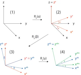
Figure 2.2: The convention upon using Euler angles to rotate between frames of ref-erence. From frame (1) a rotation by α about the z-axis, results in the frame (2). Secondly a rotation about the new y-axis through β gives frame (3). Then a final rotation through γ about the finalz-axis, results in frame (4). The convention used is that of passive rotations.

ˆ

R(α, β, γ) = ˆRz(α) ˆRy(β) ˆRz(γ) (2.58)

Figure 2.2 shows how these rotations are applied. Initially a rotation by α about the z-axis, followed by a rotation about the new y-axis through β, then a final rota-tion through γ about the final z-axis. It is important to note that different conven-tions of these rotaconven-tions exist, but the convention used in this thesis, is that of passive rotations.[98]

An operator ˆR acting on a spherical tensor can be described by:

ˆ

R(Ajm) = m0=+j

X

m0_=−j

D_mj 0_m(α, β, γ)A0_jm0 (2.59)

where D_mj0_m(α, β, γ) is a rotation matrix, the Wigner D-matrix. Therefore, upon

(41)

rank j, but different order m. The Wigner D-matrix is defined in terms of the Euler angles as [103, 104]:

Dj_m0_m(αβγ) =e−im 0_α

dj_m0_m(β)e−imγ (2.60)

where dj_m0_m are the reduced Wigner matrices which can be found in reference tables,

see Appendix A.1 [100].

Thus, for the specific case of the NMR experiment, in transforming frames from the PAS to the lab frame (L), we have:

AL_jm0 = X

m

AP_jmD_mmj 0(αP L, βP L, γP L) (2.61)

so with any spherical tensor in the PAS frame of a particular interaction we can now transform to the more general lab frame.

It is important to note that due to the interactions being considered as first order perturbations, only spin terms that commute with the Zeeman interaction, ˆIz,

are retained:

[ ˆIz,Tˆjm] =mTˆjm. (2.62)

The above equation only commutes when m= 0, meaning that in the lab frame only AL

j0 terms are retained. This is known as the secular approximation, and only holds

when first order perturbations to the Zeeman interaction are considered. Therefore:

ˆ

HL₌_AL

00Tˆ00+AL20Tˆ20 (2.63)

where AL₀₀ corresponds to the isotropic component of the particular interaction, and AL₂₀ the anisotropic component.

2.4.2 Magic Angle Spinning (MAS)

(42)

β

_RL

α

_RL

=

−

ω

_r

t

R

LAB

B

₀

Ω

_RL

[image:42.595.242.433.70.304.2]

Ω

_PR

PAS

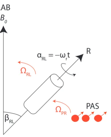
Figure 2.3: Diagram showing the orientation of the MAS rotor with respect to the external B0 field. Euler angles are shown for the transformations between the PAS to

the rotor frame, and then a further rotation to the lab frame.

NMR due to the rigidity of solids, this molecular tumbling does not occur, thus result-ing in the anisotropic component still beresult-ing present. This will lead to broadenresult-ing of the lineshapes observed, especially in the case of powered solids where a range of orienta-tions will be present, resulting in the overlap of many different anisotropic resonances. Therefore, in solid state NMR a commonly employed technique is that of Magic Angle Spinning (MAS), whereby the sample is orientated at a fixed angle to the external magnetic field and rotated about this axis, with the aim of removing this anisotropic component of the interactions.

A further transformation is now required from the PAS frame to the so called rotor frame, the rotor being the small container the sample is put into and subsequently rotated in, and finally a further transformation to the lab frame where the NMR mea-surement is taken. There are now two sets of Euler angles we need to consider:

ΩRL = (αRL, βRL, γRL) (2.64)

ΩP R = (αP R, βP R, γP R). (2.65)

(43)

of ΩRL, the user has control of γRL, enabling it to be set to zero. βRL is the angle of

the rotor with respect to the magnetic field, and αRL the rotor position, that is time

dependent, t, and also depends upon the frequency of rotation,ωr.

For the two rotations, Equation 2.61 can be written as:

AL₂₀=AP₂₀

2

X

m=−2

D2_m0(ΩRL)D0m2 (ΩP R) (2.66)

only the AL₂₀ term is important as previously mentioned, Equation 2.63. The Wigner D-matrix for the transformation from the rotor to the lab frame is given by:

D2_m0(ΩRL) =eimωrtd20m(βRL). (2.67)

Upon rotating the sample using Magic Angle Spinning, if we average over one complete rotor period, tr= 2π_ω_r then:

Z 2_ωrπ

0

eimωrt_{= 0} _if _m₆_{= 0} _(2.68)

= 1 if m= 0 (2.69)

so when m = 0, the time dependent component equates to unity after one rotation period. For all other values ofm the time dependent part becomes zero after one rotor period. Equation 2.66 becomes:

< AL₂₀>tr=A

P

20D002 (ΩP R)d200(βRL), (2.70)

where the reduced Wigner Matrix has the form:

d2₀₀(βRL) =

1 2(3cos

2_β

RL−1), (2.71)

known as the P2(cosθ) Legendre polynomial. It can be seen that upon settingβRL to

an angle of 54.74◦ this (3cos2βRL−1) term goes to zero upon averaging over one rotor

(44)

NMR being described by second rank tensors, this makes MAS a powerful tool. However, if the spectra are not acquired at an integer of a complete rotor period, as is often the case, (m 6= 0), the other terms of Equation 2.66 must be considered. Thus calculating the remaining Wigner rotation matrices under MAS the spatial term becomes:

AL₂₀=AP₂₀

1 2sin

2_β

P Rcos(2γP R−2ωrt)−

1

√

2sin2βP Rcos(γP R−ωrt)

(2.72)

these terms oscillating atωr and 2ωr are what give rise to what is known as ‘spinning

sidebands’. Upon rotation of the sample at the magic angle the powder lineshape splits up into a series of resonances separated in Hz, by the MAS frequency ωr. As ωr is

increased the intensity of these spinning sidebands decrease, ultimately disappearing when the spinning frequency is much greater than the size of the anisotropy. This leads to one resonance observed at the isotropic chemical shift.

2.4.3 Chemical Shielding

Arguably the most important internal interaction in NMR is that of chemical shielding, as it gives direct evidence on the local chemical environment. In the presence of a strong magnetic field, in the case of the NMR experiment that of B0, the magnetic

field experienced by the nuclear site can differ from the applied field. This is because of the fact that currents in the electron orbitals surrounding the nucleus induce a different magnetic field experienced at the nuclear site, i.e. so called shielding or de-shielding the nucleus. Due to the 3D nature of this electron density, the chemical shielding is described by a second rank tensor, ˜σ. The Hamiltonian describing the chemical shielding for a spin I is given by:

ˆ

(45)

As previously stated all interactions can be defined within their principal axis system (PAS), which for the shielding tensor is:

σP =      

σXX 0 0

0 σY Y 0

0 0 σZZ

      (2.74)

where capital subscripts denote the PAS frame. Upon rotation from the PAS frame of the shielding interaction into the lab frame the tensor becomes:

σL=      

σxx σxy σxz

σyx σyy σyz

σzx σzy σzz

      . (2.75)

This can then be combined with the expression for the external magnetic field. The field at the nucleus including both contribution from the shielding and the external field is then:

ˆ

B = (1−σ).B0=

     

1−σxx −σxy −σxz −σyx 1−σyy −σyz −σzx −σzy 1−σzz

            0 0 B0       =      

−σxzB0 −σyzB0

(1−σzz)B0

      . (2.76)

In the above both contributions due to−σxz and −σyz can be neglected as they

repre-sent second order contributions. This then gives the total Hamiltonian for the chemical shielding interaction as:

ˆ

Hcs=γIˆz.σzz.B0. (2.77)

An expression for σzz is then required to accurately describe this Hamiltonian:[101]

σzz(θ, φ) =σiso+

1

2∆[(3cos

2_θ₋₁₎₋_η₍_sin2_θcos₂_φ_)] _(2.78)

where the angles θ and φrepresent polar angles that arise from the rotation from the PAS to the lab frame. The three termsσiso, ∆, andη characterise the local symmetry

around the nucleus and are expressed as

σiso =

1 3(σ

P

(46)

∆ =σ_ZZP −σiso (2.80)

η= σ

P

Y Y −σXXP

∆ (2.81)

σisois the isotropic value, corresponding to the average of the diagonal elements, as the

name suggests being isotropic means it is invariant under rotations. ∆ and η are the anisotropy and the asymmetry, respectively, and give information on the local symmetry around the nuclear site. It is common practice for these three terms to be quoted as a measure of the shielding interaction, rather than the three principal components.

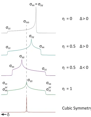
In solid state NMR the sample under observation is usually in powder form, thus all possible orientations of crystallites, hence θ and φ, are represented resulting in different chemical shielding values. A powder patten subsequently forms, spanning a range of frequencies. The distinctive lineshape of this pattern depends heavily upon the symmetry of the tensor, as shown in Figure 2.4.

As shown in Section 2.4.2 MAS can be used to remove anisotropic broadening due to first order interactions, after two successive frame rotations. This is commonly applied to remove the effect of CSA in the solid state, thus leaving a resonance with the only chemical shielding effect being from the isotropic value. The isotropic shielding is normalised with respect to a reference Larmor frequency for the observed nucleus by:

δiso =

νsample−νref

νref

×106 = σref −σsample 1−σref

(2.82)

to obtain the isotropic chemical shift δiso, which is quoted in parts per million (ppm),

and is usually what experimentalists measure. Due to the normalisation with respect to a known reference frequency, chemical shifts are independent ofB0, thus enabling a

method of comparison for spectroscopists at a wide range of field strengths.

2.4.4 Dipolar Interaction

(47)

σ

iso

σ

xx

=

σ

yy

σ

zz

σ

zz

σ

zz

σ

xx

σ

xx

σ

yy

σ

zz or

σ

xx

σ

xx or

σ

zz

σ

yy

σ

yy

η

= 0

η

= 0.5

η

= 0.5

η

= 1

Cubic Symmetry

Δ

> 0

Δ

> 0

Δ

< 0

[image:47.595.175.486.72.469.2]

δ

Figure 2.4: Chemical shift anisotropy (CSA) powder patterns, made up of randomly orientated crystallites. Lineshapes observed due to different values ofηand ∆. Bottom spectrum for the case of cubic symmetry is what is observed under MAS whereby the anisotropy is removed, using rotor-synchronised acquisition.

classical energy of the interaction between two magnetic dipoles we obtain:

ˆ HD =−

µ0

4π ¯ hγIγS

r3 ( ˆI.Sˆ−

3( ˆI.rˆ)( ˆS.rˆ)

r2 ) (2.83)

where ˆI and ˆS represent the two coupled spins, andr the distance between them. We can define a dipolar coupling constant as:

dIS =−

µ0

4π ¯ hγIγS

r3 , (2.84)

(48)

θ

= 90 °

θ

_{= 90 °}

θ

= 0 °

θ

= 0 °

d

θ

B

₀

(a)

(b)

Figure 2.5: (a) Diagram showing the orientation of the internuclear vector (θ), between two dipolar coupled spins. (b) Powdered static lineshape for dipolar coupled heteronu-clear spin pair showing the “Pake Doublet”. The “horns” representθ= 90◦, where the internuclear vector is perpendicular to B0. The humps at the end of the tail represent

θ= 0 ◦, where the internuclear vector is parallel toB0.

be a good measure of internuclear distances. The Hamiltonian represented in Cartesian tensors is given by:

ˆ

HD =−2 ˆI.D.˜ Sˆ (2.85)

in angular frequency units. Here ˆDis the dipolar coupling tensor which describes how the magnetic field at one spin is affected by the other spin, upon variation of the I-S internuclear vector in the applied field, see Figure 2.5. However, it is more useful to represent the dipolar coupling Hamiltonian in spherical tensor form. In its principal axis system it is given by:

ˆ HP

D =AP20Tˆ20 (2.86)

only the AP

20 remains due to the fact that the dipolar interaction is traceless Axx+

Ayy+Azz = 0, and axially symmetric Axx =Ayy. This has the consequence that the

dipolar interaction contains no isotropic terms, only having anisotropic contributions. In solution molecular tumbling averages away this anisotropic interaction resulting in no dipolar broadening, although relaxation effects are still experienced. Due to the lack of motion in the solid state the anisotropic term remains, with the spatial term given by:

AP₂₀=

√

Development of solid state NMR on disordered systems, from bioactive glasses to mullites

University of Warwick institutional repository: http://go.warwick.ac.uk/wrap

A Thesis Submitted for the Degree of PhD at the University of Warwick

http://go.warwick.ac.uk/wrap/66689

This thesis is made available online and is protected by original copyright.

Please scroll down to view the document itself.

Development of Solid State NMR on Disordered

Systems, from Bioactive glasses to Mullites

Scott Paul King

Department of Physics

Contents

List of Tables

List of Figures

Acknowledgments

Declarations

Abstract

Abbreviations

Chapter 1

Introduction

1.1

History of NMR

1.2

NMR of Bioactive Phosphate Glasses: Motivation

1.3

NMR of Mullite Structures: Motivation

Chapter 2

NMR Theory

2.1

Zeeman Interaction

m

−

½

½ |α>

|β>

ω

B

=

B

B

= 0

2.2

Density Operator

2.3

Hamiltonians and Interactions

2.4

Internal Interactions

z

y

x

z =

z

y

xx

x

y

z

z

x

x

y

=

y

z

=

z

x

x

y

y

R

(α)

R

(γ)

R

(β)

(1)

(2)

(3)

(4)

β

₌

_y

₌

_z

_{= 90 °}