A cylindrical magnetohydrodynamic arbitrary Lagrangian Eulerian code

(1)

University of Warwick institutional repository: http://go.warwick.ac.uk/wrap

A Thesis Submitted for the Degree of PhD at the University of Warwick

http://go.warwick.ac.uk/wrap/63693

This thesis is made available online and is protected by original copyright.

Please scroll down to view the document itself.

(2)

www.warwick.ac.uk

TITLE:A Cylindrical Magnetohydrodynamic Arbitrary Lagrangian Eulerian Code

DATE OF DEPOSIT: . . . .

I agree that this thesis shall be available in accordance with the regulations governing the University of Warwick theses.

I agree that the summary of this thesis may be submitted for publication. I agree that the thesis may be photocopied (single copies for study purposes only).

Theses with no restriction on photocopying will also be made available to the British Library for microfilming. The British Library may supply copies to individuals or libraries. subject to a statement from them that the copy is supplied for non-publishing purposes. All copies supplied by the British Library will carry the following statement:

“Attention is drawn to the fact that the copyright of this thesis rests with its author. This copy of the thesis has been supplied on the condition that anyone who consults it is understood to recognise that its copyright rests with its author and that no quotation from the thesis and no information derived from it may be published without the author’s written consent.”

AUTHOR’S SIGNATURE: . . . .

USER’S DECLARATION

1. I undertake not to quote or make use of any information from this thesis without making acknowledgement to the author.

2. I further undertake to allow no-one else to use this thesis while it is in my care.

DATE SIGNATURE ADDRESS

(3)

Lagrangian Eulerian Code

by

Thomas Goffrey

Thesis

Submitted to the University of Warwick for the degree of

Doctor of Philosophy

Physics

(4)

List of Figures

2.1 Hydrodynamical variable placement on a staggered grid. . . 12

2.2 Indexing for the four velocity vectors associated with each cell (ir,iz). 13 2.3 Indexing used for the cells associated with a node. . . 13

2.4 Indexing used for the four nodes associated with a cell. . . 14

2.5 Illustration of the primary and median meshes . . . 15

2.6 Indexing for the four corner masses contributing to the total mass of cell (ir,iz). . . 17

2.7 Indexing for the four corner masses contributing to the total mass of a node. . . 18

2.8 Indexing used for the primary mesh vectors,~ai. . . 19

2.9 Indexing and orientation for median mesh vectors. . . 19

3.1 Results for Sod’s shock tube with edge viscosity. . . 39

3.2 Initial grid for Saltzman’s piston problem . . . 40

3.3 Density contour plot for Saltzman’s piston problem at t=0.8 using edge viscosity. . . 41

3.4 Grid for Saltzman’s piston problem at t=0.8 using edge viscosity. . . 41

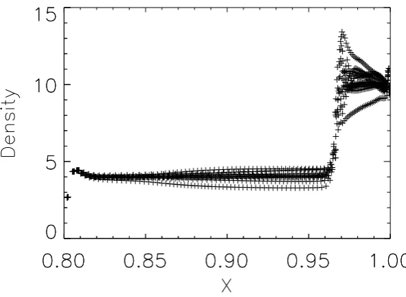
3.5 Density scatter plot for Saltzman’s piston problem at t=0.8 using edge viscosity. . . 42

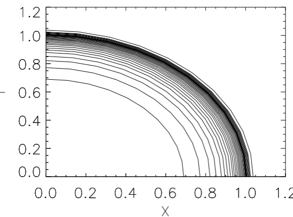
3.6 Noh’s problem on a polar grid with edge viscosity. . . 43

3.7 Density contour plot for Noh’s problem run on a Cartesian grid with edge based shock viscosity. . . 43

3.8 Grid for Noh’s problem run with edge based shock viscosity on an initially Cartesian grid. . . 44

3.9 Scatter plot of density against radius for Noh’s problem run with edge based shock viscosity. . . 45

3.10 Sod’s shock tube using tensor shock viscosity. . . 55

(10)

tensor shock viscosity. . . 56

3.12 Grid for Saltzman’s piston problem at t=0.8 using tensor shock vis-cosity. . . 57

3.13 Density scatter plot for Saltzman’s piston problem at t=0.8 using tensor shock viscosity. . . 57

3.14 Noh’s problem on a polar grid using tensor shock viscosity. . . 58

3.15 Density contour plot for Noh’s problem run on a Cartesian grid with tensor shock viscosity. . . 59

3.16 Grid for Noh’s problem run with tensor shock viscosity on an initially Cartesian grid. . . 59

3.17 Scatter plot of density against radius for Noh’s problem run with tensor shock viscosity. . . 60

3.18 Grid resulting from Sedov’s problem on a Cartesian grid. . . 61

3.19 Density contour plot for Sedov’s problem run on a polar grid with tensor shock viscosity. . . 62

4.1 Set up for cylindrical Collapse . . . 64

4.2 The vectors used to calculate CVD forces by Caramana et al. . . 67

4.3 Areas used to calculate nodal masses in AWD. . . 70

4.4 Sod’s shock tube in cylindrical coordinates. . . 75

4.5 Density contour plot for Noh’s problem run on a Cartesian grid with tensor shock viscosity, in cylindrical coordinates. . . 76

4.6 Grid for Noh’s problem run with tensor shock viscosity on an initially Cartesian grid, in cylindrical coordinates. . . 77

4.7 Scatter plot of density against radius for Noh’s problem run with tensor shock viscosity, in cylindrical coordinates. . . 77

5.1 Modes of grid motion . . . 80

5.2 The dynamical (red) and non-dynamical points (green) of a cell. . . 83

5.3 The redistribution with weightings of forces from non-dynamical points to dynamical points. . . 84

5.4 The initial forces calculated for subzonal pressures. . . 85

5.5 The intermediate forces in the rebound method. . . 86

5.6 The final forces in the rebound method. . . 87

5.7 Original force segments calculated for pressure perturbations in tri-angular subzones. . . 90

(11)

pressures. . . 92

5.9 Redistribution of forces from central non-dynamical point to nodes. . 93

5.10 Averaging of central force to nodes. . . 94

5.11 Density contour plot for Sedov’s problem att= 1.0 run on a Cartesian grid with tensor shock viscosity. . . 96

5.12 Grid for Sedov’s problem at t = 1.0 run with tensor shock viscosity on an initially Cartesian grid. . . 96

5.13 Density contour plot for Sedov’s problem att= 1.0 run on a Cartesian grid with tensor shock viscosity, in cylindrical coordinates. . . 97

5.14 Grid for Sedov’s problem at t = 1.0 run with tensor shock viscosity on an initially Cartesian grid, in cylindrical coordinates. . . 97

6.1 One dimensional remap. . . 101

6.2 Indexing used for redistribution of remap masses to nodal cells. . . . 105

6.3 Two dimensional remap. . . 107

6.4 Remapping illustrating double counting of overlap areas for swept region based remap. . . 109

6.5 Density contour plot for Sedov’s problem, using a first order remap. 114 6.6 Line plot of the density obtained along y = 0 for Sedov’s problem using a first oder remap. . . 115

7.1 Indexing used for a three dimensional cell. . . 122

7.2 Flux tube moving through a stationary grid at t = 0 (red) and one time step later, blue. . . 123

7.3 Change in flux in ignorable direction. . . 125

7.4 The initial fluxes for a cell centred remap scheme. . . 126

7.5 The development of subzonal pressures. . . 128

7.6 Dynamic flux points in an eight point cell centred remap. . . 129

7.7 Eight point cell centred remap. . . 130

7.8 Dynamic flux points of a four point cell centred remap. . . 131

7.9 Four point cell centred remap. . . 132

7.10 Initial forces for the Brio and Wu problem. . . 133

7.11 The pre-initial magnetic field can be visualised as the flux through the median mesh. ∂Xi/∂aj for each cell is calculated numerically using the edge midpoint positions as indicated. . . 139

7.12 The pre-initial magnetic field is shown to be the correct calculation of the flux through the median mesh. . . 139

(12)

of evolution through the induction equation. . . 141

7.14 Brio and Wu magnetised shock tube problem, fully Lagrangian Re-sults. 800 cells. . . 147

7.15 Brio and Wu magnetised shock tube problem, fully Lagrangian Re-sults, with compression switch active. 800 cells. . . 148

7.16 Magnetised Noh problem, run with viscosity coefficients c1 = 0.1, c2,= 0.5 Fully Lagrangian, 50x50. . . 149

7.17 Magnetised Noh problem, run with viscosity coefficients c1 = 1.0, c2,= 1.0. Fully Lagrangian, 50x50. . . 149

7.18 MHD Rotor problem, fully Lagrangian Results. 200x200. . . 151

7.19 MHD Rotor problem, fully Lagrangian until t = 0.39, then fully Eu-lerian. 400x400. . . 152

7.20 Orszag Tang Vortex, run in fully Eulerian mode. 400x400 . . . 153

7.21 Orszag Tang Vortex, run in fully Lagrangian mode until t=1.0, fully Eulerian thereafter. 400x400 . . . 153

7.22 Orszag Tang Vortex, run with Gaussian remapping function. 400x400 153 8.1 Magnetised Noh problem, run with viscosity coefficients c1 = 0.1, c2,= 0.5 in cylindrical coordinates. Fully Lagrangian, 250x1. . . 158

9.1 Overlap areas in the corner transport upwind method. . . 163

9.2 Overlap areas in an isoparametric remap. . . 167

9.3 Volume based remap for density. . . 173

9.4 Mass based remap for energy. . . 174

10.1 Results for implosion test with edge based shock viscosity. . . 177

10.2 Results for implosion test with tensor shock viscosity. . . 178

10.3 Reference solution for implosion test run with Eulerian grid motion and tensor shock viscosity. . . 179

10.4 Density plot for implosion test case, without imposed B-field. . . 183

10.5 Density plot for implosion test case, with imposed B-field, in the z-direction. . . 184

10.6 B-field plot for implosion test case, with imposed B-field, in the z-direction. . . 185

10.7 Density plot for implosion test case, with imposed B-field, in the z-direction, and reduced thermal pressure. . . 186

(13)

direction, and reduced thermal pressure. . . 187 10.9 Density plot for implosion test case, without imposed B-field, and

γ = 2.0. . . 188 10.10Density plot for implosion test case, with imposed B-field, reduced

thermal pressure, andγ = 2.0. . . 189 10.11B-field plot for implosion test case, with imposed B-field, reduced

thermal pressure, andγ = 2.0. . . 190 10.12Density plot for implosion test case, with imposed B-field, in the

z-direction, reduced thermal pressure, and compression switch active.

γ = 2.0. . . 191 10.13B-field plot for implosion test case, with imposed B-field, in the

z-direction, reduced thermal pressure, and compression switch active.

γ = 2.0. . . 192 10.14Density plot for implosion test case, with imposed B-field in the

x-direction. γ = 2.0. . . 193 10.15B-field plot for implosion test case, with imposed B-field in the

x-direction. γ = 2.0. . . 194

(14)

Acknowledgments

Thanks go first and foremost to my supervisor professor Tony Arber who has pro-vided excellent support and advice throughout this project. I must also thank Dr Chris Brady for providing useful discussions throughout this work, and for his work in extending the capabilities of Odin. Dr Keith Bennett has also provided valuable insights into numerical methods.

I would also like to thank Dr. Andrew Barlow for his advice on arbitrary Lagrangian Eulerian methods, and whose thesis provided the starting point for my own research in the field.

On a more personal note, I would like to thank my family for their encouragement over the years, without which I would not be writing this thesis. Finally I would like to thank Olivia, her guidance and patience were integral to the completion of this work.

This work acknowledges the financial support of AWE.

(15)

Declarations

I declare that this thesis has not been submitted for a degree at another university. This thesis describes the development of a numerical code, and as such borrows methods from previously published work, I declare that where such methods have been used references to the original work has been provided.

The methods to extend the hydrodynamical remap to second order, described in chapter 9 were implemented by Dr. C. S. Brady, although planned and tested in conjunction with the author. The description and development of these methods have been included for completeness as they are used in generating the results for the final results. All other methods described were implemented by the author.

(16)

Abstract

Arbitrary Lagrangian Eulerian methods are methods which seek to take advan-tage of the strengths of Eulerian and Lagrangian methods, whilst circumventing the weaknesses. This thesis discusses the development of such a code ,Odin, in two dimensions, for both Cartesian and cylindrical coordinates. Odin is capable of handling shocks through the addition of shock viscosity to the Euler equations. Furthermore the hydrodynamical scheme is expanded to include magnetohydrody-namics.

(17)

Introduction

1.1 Introduction

Whilst this thesis covers the development of a two dimensional arbitrary Lagrangian Eulerian (ALE) code, it is worthwhile discussing the merits and disadvantages of more basic methods of modelling fluid flow, before introducing the ALE methodol-ogy. The most basic methodical distinction is between pure Lagrangian and Eulerian methods. Increasing in complexity, the next method is Lagrangian remap codes, which is a hybrid method somewhere between Lagrangian and Eulerian methods, and is in fact a limiting case of ALE codes.

1.2 Timestep Control

In analysing the relative advantages and disadvantages of particular numerical schemes for hydrodynamics the question of time-step control and efficiency will be a recurrent issue, as such it is prudent to explain briefly how a timestep is chosen for (explicit) hydrodynamics. The Courant-Friedrichs-Lewy (CFL, [1]) essentially states from a physical perspective that in a given time-step no information should be able to cross more than one grid cell. For example in a one dimensional Lagrangian calculation the time-step should be calculated according to,

∆t≤ C

∆x, (1.1)

where C is the sound speed, and ∆x is the width of the cell. For a complicated grid the choice of length becomes more complicated and it is common to take some simplification, and run with the time-step at some reduced factor of the maximum allowed by the CFL condition. However, the important result remains that the

(18)

step is (neglecting higher order schemes not considered here) inversely proportional to the minimum grid spacing.

1.3 Eulerian Methods

The most basic method of modelling fluid flow is the Eulerian method (e.g. [2],[3]). In discretising the fluid in an Eulerian code, the computational cells remain fixed in space, and allow fluid to flow through it. It is important to make a distinction here, between a pure Eulerian method, in which the grid never moves, and Eulerian mesh motion, in which at the end of the time step the grid is returned to its original position.

The main advantage in using an Eulerian method is robustness. As shall be dis-cussed Lagrangian methods often struggle to complete computations when the flow becomes complex, this is not a problem for Eulerian methods. The physics within an Eulerian code is usually simpler to expand than their Lagrangian counterparts, due to the fact that the grid is known, and orthogonal. This simplicity of the grid means that at first glance the computational cost of a single time-step should be cheaper than Lagrangian codes, however in practice Eulerian codes can be dimensionally split (where fluxes along each coordinate direction are calculated and applied indi-vidually rather than simultaneously), so this advantage can be reversed.

Eulerian codes do also have disadvantages. As the grid is fixed in space they ex-perience some numerical diffusion. This can damage the accuracy of the solution, in particular shocks may become smeared across a large number of zones, however this can also reduce numerical oscillations around shock fronts.

Providing the required resolution can also be problematic for Eulerian methods. As the grid is fixed, it is necessary to provide resolution in all required areas at all times. However for a number of applications the local resolution requirement may change during the simulation; different areas may be interesting at different times. This can increased the required number of cells by orders of magnitude for Eulerian codes, thus rendering them potentially very computationally expensive.

1.4 Riemann Solvers on Eulerian Grids

(19)

such schemes [5] is only first order but higher order schemes have been developed. Whilst due to their intrinsic nature such schemes are able to capture shocks, with-out added complications such as shock viscosity, some Riemann solvers (both exact and approximate) do encounter difficulties in modelling shock reflections and addi-tional dissipative methods are needed [6]. Finally, such schemes have tradiaddi-tionally been used for Eulerian codes, although recent efforts have seen them adapted for arbitrary grids [7]. However such schemes are computationally expensive and have further complications (such as the requirement of accurate sound speed which can be problematic) and are not considered further in this work.

1.5 Lagrangian Methods

In contrast to Eulerian methods Lagrangian methods (e.g. [8]) have a mesh which is attached to the fluid. This means that no fluid flows through cell edges during the computation, the grid moves with the fluid. This has the result that the code is less diffusive, due to the fact that the grid moves with the fluid, rather than smoothing out features during advection. This grid motion also means that the method will naturally provide time dependent resolution where it is needed. As the fluid moves in one direction or piles up in an area of the domain the grid will follow it there, providing the necessary resolution.

However these advantages come at a cost, particularly robustness. Should the flow become complex the grid may begin to twist. As the grid twists (or indeed piles up in a specific location) the distance across a cell can decrease by several orders of magnitude, which consequently reduces the time step by a proportional amount. Also the grid is completely arbitrary, so implementing increasingly complex physics can become complicated.

Comparing run time and cost between Eulerian and Lagrangian methods is tricky. Lagrangian methods do not need to be directionally split, but due to the potentially complicated nature of the grid they lack simplifications that can be made in Eulerian methods. Running with identical numbers of cells a Lagrangian method will almost certainly require more time steps to complete a calculation than Eulerian methods, due to the grid concentrating itself in areas of interest. To make a fairer comparison a higher resolution Eulerian simulation should be run. In general if Lagrangian simulations are able to complete, their results arrive quicker and more accurately, but it is a big if.

(20)

not allow mass to flow between cells, and it is possible to set up the initial conditions such that cells are only one material, i.e. the grid is aligned with material interfaces. Eulerian codes will usually employ some form of interface reconstruction (e.g. [9]), but despite this, Eulerian codes are still prone to artificial mixing.

1.6 Lagrangian Remap Codes

Lagrangian remap codes (e.g. [10]) represent the middle ground between Eulerian and Lagrangian methods, and attempt to circumvent the respective problems, whilst keeping the advantages. The idea is relatively simple, carry out a single Lagrangian step, before carrying out a remap step to return the grid back to its original position. This grid motion shall be referred to as Eulerian grid motion throughout this thesis. The Lagrangian phase of a Lagrangian remap code is exactly that, and thus inher-its inher-its advantages of reduced numerical diffusion and better estimation of mixing. However as the grid is returned to its original position at the end of the time step a number of simplifications/approximations can be made without too large a drop in accuracy, thus reducing the numerical cost of such a time step.

However the remap phase does still produce numerical diffusion. The remap step comes at added computational cost, which is increased by the fact that it is often directionally split, this obviously trades off against the reduction in complexity of the Lagrangian phase.

Of course Lagrangian remap codes, due to their Eulerian grid motion do not inherit the natural resolution of Lagrangian codes, but they do inherit the robustness of pure Eulerian codes.

1.7 Arbitrary Lagrangian Eulerian Methods

(21)

too has to cope with an arbitrary grid. The question of directionally splitting the remap is discussed in later chapters.

1.8 Thesis Outline

This thesis describes the development of a single material two-dimensional arbi-trary Lagrangian Eulerian MHD code, Odin. The thesis first begins with a basic description of the discretisation and derivation of the Lagrangian phase, in Carte-sian coordinates. Chapter 3 then introduces shock viscosities, and tests two popular methods. Chapter 4 discusses the necessary changes to be made to enable Odin to run in cylindrical coordinates as well as Cartesian coordinates. Chapter 5 introduces the problem of hourglass modes, and assess a widely used method to suppress them, subzonal pressures. In practice subzonal pressures are not used in Odin.

Chapter 6 introduces a number of different remapping strategies, and discusses the implementation of a first order remap method with an ALE code. The following chapter explains how to implement ideal magnetohydrodynamics (MHD) within an ALE code, both in its Lagrangian phase, and within the context of a first order remap, before chapter 8 briefly covers how to adapt such a scheme to cylindrical coordinates.

(22)

Governing Equations

2.1 Continuous Description

2.1.1 Euler Equations, Eulerian Form

The equations governing the evolution of an ideal fluid, the Euler equations, given in their Eulerian form are:

∂ρ

∂t +∇ ·ρ~u= 0, (2.1) ∂

∂t(ρ~u) +∇ ·(~u⊗(ρ~u)) +∇P = 0, (2.2) ∂

∂t(ρeT) +∇ ·(~u(ρeT +P)) = 0, (2.3)

whereρ is the density, ~u the velocity vector,P the (thermodynamic) pressure and

eT =ei+ 1/2u2 is the specific total energy. ei is the specific internal energy, which

for an ideal gas has the form ei = P/ρ(γ−1).These are simply statements of the

conservation of mass, momentum and energy in an Eulerian frame. These are closed by an equation of state linking density, energy and pressure.

2.1.2 Tensor Review

A basic discussion of simple tensor calculus is included in appendix A.1. However some key results are repeated here. The dyadic is defined as,

A=~a⊗~b, (2.4)

where,

Aij =aibj. (2.5)

(23)

A generalised dot product is,

~n·~a⊗~b= (~n·~a)~b, (2.6)

and,

~a⊗~b·~n=

~n·~b~a. (2.7) The divergence of a rank two tensor is,

∇ ·T = ∂Tji

∂xj

, (2.8)

so that the divergence of a dyadic is,

∇ ·~a⊗~b= (∇ ·~a)~b+ (~a· ∇)~b. (2.9)

Finally the divergence theorem for tensors is,

Z

V

∂Tij...k...m ∂xk

dV =

I

s

Tij...k...mnkdS, (2.10)

where nk is the rank one covariant tensor associated with the face, and dS is the

magnitude of that face area. Applying (2.10) to a dyadic,

Z

V

∇ ·~a⊗~b=

I

s

(~a·~n)~b. (2.11)

2.1.3 Euler Equations, Lagrangian Form

As an ALE code evolves the equations in a Lagrangian frame the Euler equations must be rewritten using the Lagrangian derivative given by,

Df Dt =

∂f

∂t +~u· ∇f, (2.12)

for a general scalar f. Expanding (2.1) and using the definition of the Lagrangian derivative, (2.12),

Dρ

Dt =−ρ∇ ·~u, (2.13)

which is a mass conservation equation in the Lagrangian frame. Considering the momentum equation, (2.2), and using (2.9),

∂

(24)

Next, expanding the time derivative,

ρ∂~u ∂t +~u

∂ρ

∂t +~u(∇ ·ρ~u) +ρ~v· ∇~v=−∇P. (2.15)

However, by (2.1), the second and third terms cancel, yielding our momentum equa-tion in Lagrangian form,

ρD~u

Dt =−∇P. (2.16)

For a scalar and a vector, the product rule states,

∇ ·(f~a) =~a· ∇f+f∇ ·~a, (2.17)

so it is possible to expand and rewrite (2.3),

∂

∂t(ρeT) +ρeT (∇ ·~u) +u~· ∇(ρeT) =−∇(~uP), (2.18)

and by using (2.12),

DρeT

Dt =−∇ ·(~uP)−ρeT∇ ·~u. (2.19)

Once again, expanding the derivative,

ρDeT Dt +eT

Dρ

Dt =−∇ ·(~uP)−ρeT∇ ·~u, (2.20)

noting (again by using (2.13)) that the second terms on each side cancel, an equation for the Lagrangian evolution of total energy is obtained,

ρDeT

Dt =−∇ ·(~uP). (2.21)

It is possible to recast (2.21) in terms of specific internal energy,ei,

ρ

Dei

Dt +

1 2

Du2 Dt

=−∇ ·(~uP), (2.22)

and then applying the product rule (in the form of (2.17)) and the chain rule,

ρDei Dt +ρ~u·

D~u

Dt =−~u· ∇P −P∇ ·~u, (2.23)

and finally using (2.16) to cancel the second term on the left hand side with the first on the right a final energy equation in the Lagrangian frame is acquired,

ρDei

(25)

2.1.4 Reynolds Transport Theorem

Reynolds Transport Theorem for fluid parcels is a statement of the Leibniz integral rule. It is given by [12],

D Dt

Z

Ω(t)

~ f dV =

Z

Ω(t)

∂ ~f ∂tdV +

Z

∂Ω(t)

(~v·~n)f dA,~ (2.25)

where the integration is carried out over a fluid volume,Ω(t) bounded by a surface,

∂Ω(t). The vector, ~n is the unit normal vector to that surface. The velocity ~v

need not be the fluid velocity, it is simply the velocity of the bounding surface. Before using the theorem on the Lagrangian form of the Euler equations, this can be manipulated into a more useful form. Using first the generalised dot product, (2.6) (which has been shown in appendix A.1 to be equivalent to the contraction (A.7)),

D Dt

Z

Ω(t)

~ f dV =

Z

Ω(t)

∂ ~f ∂tdV +

Z

∂Ω(t)

~n·~v⊗f~

dA, (2.26)

Now using the divergence theorem for tensors (2.10), and the definition of the di-vergence of a rank two (contravariant) tensor, (2.8),

D Dt

Z

Ω(t)

~ f dV =

Z

Ω(t)

∂ ~f ∂tdV +

Z

Ω(t)

∇ ·~v⊗f~dV. (2.27)

Expanding this using (2.9),

D Dt

Z

Ω(t)

~ f dV =

Z

Ω(t)

"

∂ ~f

∂t +~v· ∇ ~

f+f~(∇ ·~v)

#

dV. (2.28)

Using (2.12) yields our final form of the Reynolds Transport Theorem,

D Dt

Z

Ω(t)

~ f dV =

Z

Ω(t)

"

D ~f Dt +

~ f(∇ ·~v)

#

dV. (2.29)

2.1.5 Integral form of the Euler Equations

(26)

(2.13):

Z

Ω(t)

Dρ

DtdV =−

Z

Ω(t)

ρ∇ ·~udV, (2.30)

From (2.29) it follows,

D Dt

Z

Ω(t)

ρdV = 0. (2.31)

It will be useful to define volume averaged quantities as,

¯

f = 1

V

Z

Ω(t)

f dV. (2.32)

Similarly to (2.32) a mass averaged quantity will be introduced,

˜

f = 1

M

Z

Ω(t)

f ρdV, (2.33)

Using (2.32), (2.31) can be rewritten as,

D DtρV¯ =

D

DtM = 0, (2.34)

where M = ¯ρV is the cell mass. This is a familiar result, that the mass in a Lagrangian cell is constant. Moving onto (2.16), and integrating,

Z

Ω(t)

ρD~u

DtdV =−

Z

Ω(t)

∇P dV. (2.35)

Considering first the left hand side,

Z

Ω(t)

ρD~u DtdV =

Z

Ω(t)

D

Dt(ρ~u)−~u Dρ Dt dV = Z

Ω(t)

D

Dt(ρ~u) +~uρ(∇ ·~u)

dV

= D

Dt

Z

Ω(t)

ρ~udV,

where in the last step (2.29) has been used. Use (2.33) this can be rewritten as,

D Dt

Z

Ω(t)

ρ~udV = D

DtM

˜

(27)

and by applying the divergence theorem to the right hand side and using (2.36) the final integral equation for the momentum update in Cartesian coordinates is obtained,

MD~u˜ Dt =−

Z

∂Ω(t)

P ~dS. (2.37)

It is desirable to apply the same method to define a model for updating the energy equation. However as will be shown such a simple form cannot be obtained without some questionable steps. In fact Odin uses a compatible energy update [13] in place of such a model. The discussion that follows is provided for completeness. As with the momentum equation it is possible to rearrange the left hand side of the integral of the energy equation, (2.24),

MDe˜i Dt =−

Z

Ω(t)

P∇ ·~udV. (2.38)

The pressure relates to density and specific internal energy through the equation of state. As finite volume codes only ever model the volume/mass average of such quantities, ¯ρand ˜ei, it follows that only a volume average pressure, ¯P is ever known.

Thus it is possible to remove the pressure from the integral, now being explicit that only an average pressure value is known, to yield an energy update of the form,

MDe¯i Dt =−

¯

P

Z

Ω(t)

∇ ·~udV =−P¯

Z

∂Ω(t)

~u·dS.~ (2.39)

However in place of (2.39) a compatible energy update is used to ensure exact energy conservation. This method shall be explained in a later section. In this section ¯f

(28)

2.2 Discrete Description

2.2.1 Hydrodynamical Variable Placement

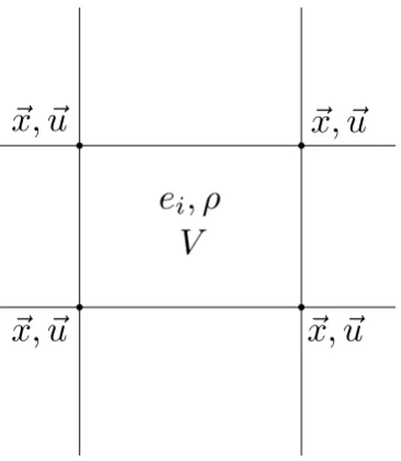
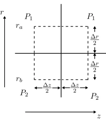
[image:28.595.235.418.243.453.2]

Before discussing the details of the numerical scheme within Odin it is necessary to define the placement of each variable on the grid. Odin employs a staggered grid hydrodynamic scheme, where variables such as density, volume and internal energy are defined at cell centres, and variables such as velocity and position are defined at nodes. This is demonstrated by figure 2.1.

Figure 2.1: Hydrodynamical variable placement on a staggered grid.

(29)

[image:29.595.229.396.491.661.2]

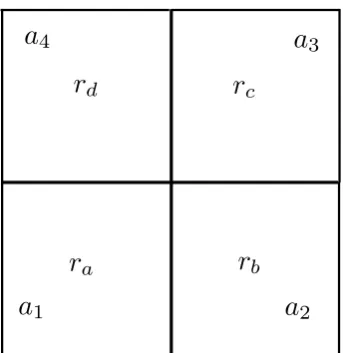
coordinate system. In order to calculate forces for each node, the four contributions

Figure 2.2: Indexing for the four velocity vectors associated with each cell (ir,iz).

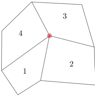
from each of its four connected cells will need to be considered. When doing so it is useful to define and retain an indexing. The four cells associated with each node are numbered 1-4 in an anticlockwise manner, starting bottom left, this is demonstrated by figure 2.3. A similar indexing is used for the nodes associated with each cell, this

Figure 2.3: Indexing used for the cells associated with a node (highlighted in red).

(30)

of each cell, which once again are defined in an anticlockwise manner, this time starting at the bottom edge.

Figure 2.4: Indexing used for the four nodes associated a cell. The nodes are highlighted in red. The indexing for the cell edges is also denoted by numbers, and the cell edge midpoints have been highlighted blue for clarity.

2.2.2 Compatible Energy Update

A compatible energy update, [13], may be viewed as choosing a discretisation which always analytically conserves energy. Essentially compatibility involves the calcula-tion of the forces used for the update of the momentum equacalcula-tion, then replacing the normal energy update equation with a combination of those forces and the half time step velocities, in such a way that the total energy is conserved over the full timestep.

Definition of Corner Masses

(31)

and the nodal mass,MP, are considered constant.

The result of this is that there are two sets of boundaries over which no mass flows, the boundaries of the cells (the primary mesh) and the boundaries of the nodes (or the median mesh). The median mesh is the mesh defined by connecting the midpoints of each cell edge. Both meshes are demonstrated by figure 2.5.

Figure 2.5: The two meshes are illustrated. The primary mesh (solid lines) is defined by the connection of nodes with their nearest (in logical space) neighbours. The median mesh (dotted lines) is defined by the connection of the midpoints of cell edges. The median mesh segments used to define the volume associated with single node have been highlighted red. As both nodal and cell centred masses are assumed to constant, no mass can flow through either mesh.

Thus two sets of constant masses are defined, however their sum must be equal,

X

p

Mp = X

z

Mz, (2.40)

(32)

masses that are referred to as corner masses, and shall be denoted mi_j, where the indexing is explained in the following section.

It should be stressed that in fixing the subzonal masses as constant masses associated with the intersection of the primary and median mesh a finite volume numerical model is being defined. The centre of a zone is not itself a Lagrangian point, and the assumption that no mass flows across the median mesh is again simply a step in defining a numerical model. The finite volume model will converge to the correct limit, but is not one derivable from the fluid equations. This is why the step to use a compatible energy update in place of the integral energy equation is important. As will be shown this numerical model does exactly conserve mass, energy and momentum. To calculate the mass of a zone or node the following summations (keeping for now the notation of [13]) are carried out,

Mz=X

p

mz_p, (2.41)

and,

Mp=X

z

mp_z. (2.42)

where in (2.41) the summation is carried out over all points associated with the zone (see figure 2.4) and in (2.42) over all zones associated with a point (see figure 2.3). To be clear, mz_p = mpz, but summations are always carried out with respect

to the lower index. To summarise the mass of a zone is calculated by summing over all corner masses with that fixed label z, and to calculate the nodal mass the summation is carried out over fixed label p.

Clearly if there arenr×nz cells there will be 2nr×2nz corner masses. Within Odin the corner masses (m) are given two indices,iandj, so

MCell(ir, iz) =

2ir X

i=2ir−1 2iz X

j=2iz−1

mi,j, (2.43)

and,

MN ode(ir, iz) =

2ir+1

X

i=2ir

2iz+1

X

j=2iz

mi,j. (2.44)

(33)

Figure 2.6: Indexing for the four corner masses contributing to the total mass of cell (ir,iz).

Compatible Formulation

Before using the corner masses described in the previous subsection, some grid vectors must be defined. There are two sets of grid vectors. For each cell there are associated eight primary grid vectors, two to each cell face. These are equal in magnitude to half the area of that cell face and point in an outward normal direction with respect to the cell and it’s face. The indexing for these is illustrated by figure 2.8.

(34)

Figure 2.7: Indexing for the four corner masses contributing to the total mass of node (ir,iz). For clarity the line segments defining the nodal cell have been highlighted in red.

case, and in three dimensions it will be an area, as such it is referred to as an area. The direction and indexing of the median mesh vectors are defined by figure 2.9.For a Cartesian codeS~1 =−S~3, however this is not the case for a cylindrical code, where

the vectors may be defined at a different radial coordinate.

Consider the integral form of the momentum equation in Cartesian coordinates (2.37),

Mp

D~vp

Dt =−

Z

V

∇P dV =− I

δS

P ~ndS=X

z

~

f_zp. (2.45)

In the final step a similar notation to that of corner masses has been employed, where the summation is carried out over all (yet to be defined) corner forces associated with the node, p. In the context of (2.45)f~zp is the force contribution due to pressure

(35)

Figure 2.8: Indexing used for the primary mesh vectors,~ai.

Figure 2.9: Indexing and orientation for median mesh vectors. The median mesh itself is shown by the dotted line. This diagram is used to define directions, so thatS~1 = 0.5 (y1−yc, xc−x1) and S~3 = 0.5 (y3−yc, xc−x3), wherexc, yc are the

coordinates of the cell centre, andxi, yi are coordinates of cell edges, with indexing

(36)

pressure gradient. Indeed a corner force is not the total force on a corner mass, but the total force on a single node from a single zone.

Corner forces are the four force contributions of a cell to each of its nodes. As forces are carried out by calculating the integral (2.37) around the median mesh the forces from each of the four cells associated with each node can be written as four discrete force contributions. These discrete forces are known as corner forces, and use the same indexing system as the corner masses.

To examine the total energy of the domain two sums must be carried out, over nodes and cells,

ET = X

Cells

Mzez+ X

N odes

Mpvp2

2 , (2.46)

where ez is the specific internal energy of the cell. The total energy across the

domain is,

ET = X

z

Mzez+ X

p

Mp

v_p2

2 . (2.47)

Taking the total derivative with respect to time, and using the Lagrangian nature of both the cell masses, and the nodal masses,

D DtET =

X z Mz Dez Dt + X p X z ~ f_zp·~vp

=X z Mz Dez Dt + X p ~ f_zp·~vp

!

+X

i

~

fbd,i·~vbd,i. (2.48)

The final term in (2.48) represents contributions from boundary forces, which will be neglected for the remaining part of this discussion. Now in order for the contri-butions from the cells to total zero, the following condition is clear,

Mz

D

Dtez =−

X

p

~

f_pz·~vp. (2.49)

(37)

update of internal energy gives the following,

Mz

Dez

Dt =−

X

p

~vp·f~pz

=−Pz h

~ S1−S~4

·~v1+

~ S2−S~1

·~v2+

~ S3−S~2

·~v3

+

~ S4−S~3

·~v4

i

=−Pz[(~a8+~a1)·~v1+ (~a2+~a3)·~v2+ (~a4+~a5)·~v3

+ (~a6+~a7)·~v4]

=− I

∂S

Pz~n·~vdS

=− Z

V

Pz∇ ·~vdV. (2.50)

In the first step of (2.50) vector addition has been used; it should be stressed that this equality is only true for Cartesian coordinates. The second step has carried out a piecewise constant boundary integral, and the final step is just the application of the divergence theorem.

Although (2.50) shows that compatible discretisation occurs naturally for Cartesian coordinates in any dimension this is not true for other coordinate systems, where the third equality does not hold. As such (2.51) is adopted as the canonical form of the internal energy update in both Cartesian and cylindrical coordinate systems,

MzDei Dt =−

4

X

i=1

~

fi·v~i, (2.51)

where the forces are the same forces used to update the velocity components of the nodes,

MpDvx Dt =

4

X

i=1

fx,i. (2.52)

The implementation of a compatible energy update can be viewed as the replacement of the continuous energy change, defined as the product of pressure and change in volume, with a discretised total work rate. The discrete forces are combined with the discrete velocities to form a discrete rate of work, and thus energy change of the cell.

(38)

(2.48) over a single time step yields,

X

z

Mz∆ez+ X

p

Mp∆

v_p2

2 =

X

z

Mz∆ez+ X

p

Mp~vnp+1/2·∆~vp = 0, (2.53)

where ∆ represents the change in quantities between time steps n and n+1. The discrete (in both time and space) form of the momentum update is

Mp∆~vp = X

z

~

f_zp(n+1/2)∆t, (2.54)

where f~zp(n+1/2) represents a time centred force. Applying this and changing the

order of the resulting double summation,

X

z "

Mz∆ez+ X

p

~v_pn+1/2·f~_pz(n+1/2)∆t

#

= 0, (2.55)

yields the final fully discretised form of the compatible energy update,

∆ez =− X

p

~

f_pz·~vn_p+1/2∆t/Mz. (2.56)

Additional Forces

The compatible framework is a very flexible one that allows new (hydrodynamical) forces to be added in an energy conserving manner. Any force may be specified directly as a force on the nodes and (2.56) provides an energy conserving framework to calculate the resulting change in internal energy. This will prove a particularly useful tool in specifying shock viscosity forces and calculating the resulting heating. It is also worth noting that it is possible to reverse engineer such a process where some heating mechanism may be specified, and the necessary energy conserving forces may be calculated using the compatible framework.

There are a few notable exceptions. The first is the force resulting from the addition of a B-field which has no effect on the internal energy, the forces here provide a transfer of energy between the magnetic and kinetic energies. Secondly in the case of gravity (2.47) must be modified as,

ET ,cell =Mzez+ X

p

mz_p v

2

p

2 +gyp

!

(39)

whereyp is the height of the node and g is the strength of the gravitational field, to

account for the additional gravitational force,

~

fgrav =−Mpgy.ˆ (2.58)

To show energy is still conserved, consider only the additional terms arising from the inclusion of a (constant) gravitational acceleration,

D Dt

X

p

Mp~vp2

2 +gyp =

X

p

Mp~vp·

D

Dtv~p+gMp D Dtyp

=X

p

Mpvp,y(−g) +Mpvp,y

= 0. (2.59)

Here it is assumed gravity acts in the negative y-direction, although a similar result is obtained for a general gravitational field, as long as the definition of gravitational potential is correctly adjusted.

2.3 Boundary Conditions

In order to calculate forces on nodes along the boundary of the domain, as well as to carry out a remap (see Chapter 6, Chapter 9) it is necessary to define two ghost values for each variable external to the domain. The values are set according to boundary conditions. Throughout this work the only boundary conditions applied will be periodic or reflective. For simplicity these will be explained in a one dimen-sional context, application to a second dimension is trivial. The grid size is assumed to equalncells.

2.3.1 Hydrodynamical Variables

When using a periodic boundary condition, the density ghost values are applied as,

ρ0 =ρn,

(40)

for the left hand boundary, and,

ρn+1 =ρ1,

ρn+2 =ρ2, (2.61)

for the right hand boundary. The specific internal energy is applied in an analogous manner. For the velocity components the indexing is changed slightly, due to grid staggering,

~v−1 =~vn−1,

~v−2 =~vn−2, (2.62)

for the left hand boundary, and,

~vn+1 =~v1,

~vn+2 =~v2, (2.63)

for the right hand boundary. Finally it is important to enforce,

~vn=~v0. (2.64)

For reflective boundary conditions, the important principle is that no material is permitted to flow through the boundary. Considering a reflective boundary in the x-direction,

vx,0=vx,n = 0. (2.65)

The other variables are calculated to be consistent with this,

ρ0 =ρ1,

ρ−1 =ρ2,

ρn+1=ρn,

(41)

for density, and similarly for energy. The y-velocity is calculated as,

vy,−1 =vy,1,

vy,−2 =vy,2,

vy,n+1 =vy,n−1,

vy,n+2 =vy,n−2. (2.67)

The y-velocity along the boundary is allowed to evolve as any other point, with forces calculated using the other boundary values. Finally the other boundary values for the x-component of the velocity are defined,

vx,−1=−vx,1,

vx,−2=−vx,2,

vx,n+1 =−vx,n−1,

vx,n+2 =−vx,n−2. (2.68)

This set of boundary conditions allow the first set of boundary values in each di-rection to be updated during the predictor step in a consistent manner, without the need for an additional application of the boundary conditions. For reflective boundary conditions in the y-direction the roles of the x and y components of the velocity are interchanged. The scalar quantities are unchanged.

It is also necessary to apply boundary conditions to the grid positions. For reflective boundary conditions the following equations should be used,

x−1 =x0−(x1−x0) = 2x0−x1,

x−2 =x0−(x2−x0) = 2x0−x2,

xn+1 =xn+ (xn−xn−1) = 2xn−xn−1,

xn+2 =xn+ (xn−xn−2) = 2xn−xn−2, (2.69)

and,

y−1 =y1,

y−2 =y2,

yn+1 =yn−1,

(42)

For periodic boundary conditions the following boundary conditions should be used,

x−1=x0−(xn−xn−1),

x−2=x0−(xn−xn−2),

xn+1 =xn+ (x1−x0),

xn+2 =xn+ (x2−x0), (2.71)

and,

y−1 =yn−1,

y−2 =yn−2,

yn+1 =y1,

yn+2 =y2. (2.72)

finally, being sure to enforce,

y0=yn, (2.73)

and,

x0=xn. (2.74)

2.3.2 Polar Grids

(43)

components are,

vy,i,−1 =−vy,i,1,

vy,i,−2 =−vy,i,2,

vy,i,n+1 =vy,i,n−1,

vy,i,n+2 =vy,i,n−2. (2.75)

Here it has been assumed the velocity (and later the position) is indexed (i, j). These statements apply for alliand j. The x-component is calculated as,

vx,i,−1 =vx,i,1,

vx,i,−2 =vx,i,2,

vx,i,n+1 =−vx,i,n−1,

vx,i,n+2 =−vx,i,n−2. (2.76)

Velocity components normal to the boundaries are forced to be zero,

vy,i,0= 0, (2.77)

and,

vx,i,n= 0. (2.78)

The velocity component tangential to the boundary are allowed to evolve as any other interior point. For the logically left hand boundary, the velocity components are given by,

vx,−1,j =−vx,1,j,

vx,−2,j =−vx,2,j,

vy,−1,j =−vy,1,j,

vy,−2,j =−vy,2,j. (2.79)

The velocities at the origin are forced to be equal to zero,

(44)

For the logically right, or outer radial boundary the following boundary conditions are applied,

vx,n+1,j =vx,n−1,j,

vx,n+2,j =vx,n−2,j,

vy,n+1,j=vy,n−1,j,

vy,n+2,j=vy,n−2,j, (2.81)

whilst velocities on the outer radial limit are calculated normally, using the values from other boundary conditions to calculate forces.

Grid positions are done in a similar, consistent manner. Firstly the points on the inner radial boundary are forced to remain at the origin,

x0,j =y0,j = 0.0 (2.82)

Positions on the inner radial boundary are given as,

x−1,j =−x1,j,

x−2,j =−x2,j,

y−1,j =−y1,j,

y−2,j =−y2,j. (2.83)

Positions on the outer radial boundary are updated according to the respective velocity values, whilst beyond this the positions are given by,

xn+1,j= 2xn,j −xn−1,j,

xn+2,j= 2xn,j −xn−2,j,

yn+1,j = 2yn,j −yn−1,j,

yn+2,j = 2yn,j −yn−2,j. (2.84)

For the logically up boundary the positions are given as,

xi,n+1 =−xi,n−1,

xi,n+2 =−xi,n−2,

yi,n+1 =yi,n−1,

(45)

whilst enforcingxi,n= 0.0 and allowingyi,nto update according the velocity in that

position. The positions for the logically lower boundary are given by,

xi,−1 =xi,1,

xi,−2 =xi,2,

yi,−1 =−yi,1,

yi,−2 =−yi,2, (2.86)

whilst enforcing yi,0 = 0.0 and updatingxi,0 according to the velocity in that

posi-tion.

Finally, using periodic boundary conditions it is possible to model an entire (infi-nite) cylinder, by linking the logically upper and lower boundaries. The method for this remains the same as for periodic boundary conditions on a standard grid, except the positions are now given by,

xi,−1 =xi,1,

xi,−2 =xi,2,

yi,−1=yi,1,

yi,−2=yi,2, (2.87)

and,

xi,n+1 =xi,n−1,

xi,n+2 =xi,n−2,

yi,n+1=yi,n−1,

yi,n+2=yi,n−2, (2.88)

whilst enforcing,

xi,0=xi,n, (2.89)

and,

(46)

Shock Viscosity

3.1 Introduction

In an ideal fluid a shock is a discontinuous jump in velocity, density and pressure. However in a non-ideal fluid dissipative effects act to smear the discontinuity over a finite distance. In numerical modelling shock viscosity acts in a dissipative manner to enable the numerical study of situations involving such phenomena. Early shock viscosities acted as a scalar pressure added only in cells which were judged to contain a shock. As such the momentum equation is modified to,

ρD~v

Dt =−∇(P+Q), (3.1)

where Q is the shock viscosity. Von Neumann and Richtmeyer [14] were the first to introduce such a concept whilst modelling the propagation of shocks in a one-dimensional, inviscid fluid. Often referred to as the quadratic viscosity term it had a general form of,

Qquad=c2qρ(∆x)

2

∂~v ∂x

2

, (3.2)

where ∆x is the width of the cell in question, and cq is a dimensionless constant

used to control the magnitude of the shock viscosity, which was set to zero when the velocity gradient was greater than or equal to zero (when the cell was expanding). Landshoff [15] introduced what is known as a linear viscosity term,

Qlinear =clρ∆xCs

∂~v ∂x

, (3.3)

where here Cs is the local sound speed and cl is another dimensionless constant

used to control the magnitude of the linear shock viscosity. He recommended a

(47)

combination of the two terms,

QT ot=QLinear+QQuad. (3.4)

The size of these constants remained arbitrary and problem dependent (although both must be positive during compression, and set to zero in expansion), until the work of Kuropatenko [16], later repeated by Wilkins [17]. Kuropatenko considered the Hugoniot relations and using an ideal gas equation of state derived an expression for the pressure jump across a shock:

P1−P0=

γ+ 1

4 ρ0(∆v)

2

+ρ0|∆v|

"

γ+ 1 4

2

(∆v)2+C_s,2₀

#1/2

. (3.5)

What is evident here is that the early a posteriori efforts of Von Neumann and Richtmeyer, and Landschoff, were acting to try and fulfil the requirements of shock physics; the early artificial (shock) viscosities were acting to provide a pressure jump across the shock. The pressure jump provided by (3.5) is of the form of (3.4), a combination of linear and quadratic forms. Kuropatenko also noted that in the limit of small and large (∆v)2, relative toCs,0, linear and quadratic terms like (3.2) and

(3.3) respectively are recovered. The pressure jump given by (3.5) shall be used in the definition of shock viscosities and will be denoted,

qkur =

γ+ 1

4 ρ0(∆v)

2₊_ρ 0|∆v|

"

γ+ 1 4

2

(∆v)2+C_s,2₀

#1/2

. (3.6)

3.2 Edge Based Shock Viscosity

Odin contains two (optional) types of shock viscosity, the first of which is the edge based shock viscosity developed by Caramana et al [18]. Following the methodology of Schulz [8], Caramana et al [18] set out a number of physical qualities that are desirable for a shock viscosity to possess. It is this set that shall be considered in this work.

3.2.1 Requirements of Shock Viscosity

The five requirements of shock viscosity outlined by Caramana, and now used as a standard set are,

(48)

2. Galilean Invariance

3. Self-similar motion Invariance 4. Wave front Invariance

5. Viscous Force Continuity

Dissipativity is simply the requirement that the shock viscosity must always act to decrease kinetic energy and thus increase internal energy. This will sometimes be referred to as the viscous heating requirement. Shock viscosity in Odin is imple-mented within the compatible framework, so the sum of the viscous contributions to the change in internal energy must always be positive.

The remaining four requirements are all in some way connected to the identifica-tion of regions where the shock viscosity should act. In previous discussions the dimensionality of the problem has been limited to one, and thus identifying a shock has been limited to considering the (one dimensional) velocity gradient. When the velocity gradient across the cell is negative the cell is being compressed and the viscosity switches on, in regions of a positive gradient the viscosity is switched off. Galilean invariance requires that the shock viscosity vanishes smoothly as the ve-locity becomes constant. Put more simply the viscosity must not change under the addition of a uniform velocity field. Such a requirement was also used by Schulz. Self similar motion invariance requires the viscosity to not act in cells undergoing rigid rotation or uniform contraction. This condition is actually split into two condi-tions in Schulz’s work. Uniform contraction (or expansion) over the entire medium is considered a reversible process. Most importantly (regardless of discussions of entropy change) shock viscosity should only account for shock heating, so a shock viscosity should be independent of such motion. Rigid rotation was Shultz’s fourth requirement, and in fact was not fulfilled by his work. He linked this to his failure to conserve angular momentum. Such a motion is not a shock, and shock viscosity should not respond to it. Both rigid rotation and uniform contraction are considered jointly under the self similar motion invariance requirement.

Wave front invariance simply requires that the shock viscosity has no effect along a line of constant phase. Finally viscous force continuity requires that viscous forces go to zero and remain so in the transition from compression to expansion.

3.2.2 Definition of Edge Based Shock Viscosity

(49)

than as a scalar which when acted upon by the gradient operator would become a force. The form of the force is,

~

f_ivisc=qkur×(1−ψ)

∆~vi·S~i

ˆ

∆~vi, (3.7)

on the condition that

∆~v·S~

≤ 0 and zero otherwise. This condition needs ex-panding upon. Within the compatible framework, [13], forces are calculated around the median mesh of each node, and these forces are then used in place of a PdV energy update. As each median mesh segment of the cell is in contact with two nodal cells, to which it applies equal and opposite forces it is possible to re-write the compatible internal energy update, (2.51),

MDei Dt =−

4

X

i=1

~

f_i0·∆v.~ (3.8)

Here f~_i0 = PzS~i is the force associated with median mesh segment i, and ∆v~ is

the velocity difference along the cell edge to which the median mesh segment is connected so that,

~

∆vi=~vi−~vi+1. (3.9)

The definition is cyclical around the cell so that,

~

∆v4 =~v4−~v1. (3.10)

As the compatible energy update is used in terms of a PdV work, what (3.8) yields is a compatible calculation of the change of volume of the cell,

dV =

4

X

i=1

~

Si·∆v~ idt. (3.11)

This is the motivation for the dot product which triggers the shock viscosity of (3.7). The change in cell volume has been decomposed in terms of the four primary mesh cell edge contributions. It has already been stated that shock viscosity should act in areas of compression, and (3.11) has provided compression switches for each edge. Explicitly, when any of the four components of (3.11) are negative the edge in question is acting to reduce to volume of the cell and the viscosity along this edge should switch on, hence the concept of edge based viscosity. Thus numerically compression and expansion along an edge are defined.

(50)

fact it is illustrative to follow the method of [18] and visualise these forces as been associated with the triangles formed by the edges and cell midpoint. Each edge force acts as an equal and opposite force on each of it’s nodes in order to oppose the compression of the edge.

The compatible methodology requires that forces are defined in terms of corner forces. In combining the edge based viscous force with the compatible method Caramana used the viscous heating requirement in conjunction with the fact that thatf~∼ −∆~ˆv. Thus to ensure that the heating term is positive, the rate of viscous work was defined as f~edge · −∆v~ and is thus positive definite. In Odin, to bring

edge viscosity fully in line with the compatible framework the viscous corner force is coded as:

~

f_visccorner,i=−f~_visci−1+f~_visci . (3.12) This has the same total effect as the original formulation, but is now explicitly defined in terms of corner force contributions. This force re-distribution is the reverse method used to decompose PdV work in terms of median mesh contributions, and has the effect that the heating from edge viscosity can be written in the form,

MDei Dt

visc

=−X i

~

f_visccorner,i·~vi. (3.13)

3.2.3 Viscosity Limiters

In (3.7) ψ is used but not defined, it is the viscosity limiter. The purpose of the limiter function in one dimension is to act to turn off the viscosity where the second derivative of the velocity is zero, but without a direct calculation of the second derivative. This will fulfil the self similar motion requirement of the shock viscosity. In multiple dimensions Caramana showed that for a correct choice of viscosity limiter the third and fourth requirements outlined for shock viscosity are fulfilled. The limiter function for an edge, i, is defined as:

ψi =max[0, min(0.5 (rl,i+rr,i),2rl,i,2rr,i,1)], (3.14)

whererr,i and rl,i are right and left velocity ratios, defined as:

rl,i=

∆ ~vi+1·∆v~ˆi

∆ ~xi+1·x~ˆi

/|∆~vi|

|∆ ~xi|

(51)

and,

rr,i =

∆ ~vi−1·∆v~ˆi

∆ ~xi−1·x~ˆi

/|∆~vi|

|∆ ~xi|

. (3.16)

There are similar formulae for all edges. It is worth noting the suggestion from Caramana that should the effective edge CFL-like condition |∆ ~vi|

|∆ ~xi|∆t be less than

round off the both of the edge ratios should be set to unity, thus turning off the shock viscosity and reducing numerical noise.

3.3 Time step limiting in Conjunction with Shock

Vis-cosity

The preceding section provides enough information to construct a shock viscosity and how to implement it within a finite volume compatible hydrodynamics scheme. However one subtle part, which is often overlooked remains unconsidered. As the shock viscosity alters the equations of the system it’s clear that it should also alter the stable time step calculation of the system, however there has been little consensus over the exact manner of the alteration. All methods define a generalised sound speed, based upon the combination of thermodynamic pressure and an equation of state with (possibly part of) the shock viscosity. One such method [11]is:

C_s,gen.2 =C_s,2₀+2Q

ρ . (3.17)

WhereCs,0 is the normal equation of state based sound speed, and Qis some scalar

part of the shock viscosity. In the original paper outlining edge based viscosity Caramana mentioned the use of a generalised sound speed, but not it’s exact form. However in a later paper [19] where a vorticity damping term is added to the original edge based viscosity the authors review the method, and although a simplified ver-sion of the edge viscosity is presented by comparison of that with (3.7) an equivalent generalised sound speed may be derived:

Cs,gen.= Cs,20+Cq,edge2 (1/2)

, (3.18)

where,

C_q,edge2 = qkur

ρ (1−ψ). (3.19)

This gives a generalised sound speed for each edge, and the most restrictive gener-alised sound speed for each cell is used to calculate a stable time step.

(52)

in the presence of shock viscosity exist, so it is useful to examine the problem more explicitly in the limiting case of cold (zero internal energy) shock compression. As a number of standard test cases for shock viscosity have the initial condition of zero internal energy, this is a relevant case to consider.

3.3.1 Cold Compression of a single cell

Consider a simplified test case on a uniform grid, density is set to unity everywhere and internal energy zero. As previously mentioned this is not dissimilar to a number of standard test cases. Without loss of generality we can assume the cell under consideration is undergoing compression due to the motion of just one of its edges. In the more general case the motion would be considered on an edge by edge basis, and similar to before the most restrictive∆twould be used. Let us further assume that the shock viscosity in use is that of (or similar to) the edge based viscosity previously defined. However it is useful to rewrite it as,

~

f =−qKur

|∆~v|(1−ψ)

~ ∆vi·S~i

_ˆ

~

∆v. (3.20)

This can be written in a more simple form,

~

f =−k∆~v, (3.21)

where,

k= qKur

|∆~v|(1−ψ)

∆~v·S~. (3.22) Assuming the edge being compressed is that defined by nodes 2 and 3, and using (3.8)the rate of work on the cell is given by,

W =k∆v~2

2

=k(v~2−v~3)2. (3.23)

Clearly, this is positive definite. However, like in many other codes Odin only calculates the viscous force at the start of the time step, or the predictor level. So in the fully (both time and space) discretised situation the true rate of work is,

W =k ~∆v₂n·∆vn₂~+1/2. (3.24) This is positive if and only if,

SIGN

~ ∆vn₂

=SIGN

~ ∆vn₂+1/2

(53)

In the limit of zero internal energy, we can rewrite the half time step velocity jump us-ing the masses associated with the nodes in question, and the viscous forces present:

~

∆v₂n+1/2 =v~₂n−k∆t ~∆v n

2

2M2

−v~₃n−k∆t ~∆v n

2

2M3

, (3.26)

but in a uniform grid and density set up M2 = M3 = ρ∆x∆y and (3.26) can be

rewritten as,

∆vn₂+1/2 ∆vn

2

=

1−k∆t

M2

. (3.27)

In this final step the vector notation on the velocity jumps as been dropped. In a one dimensional case this step is trivial, in a multidimensional case a coordinate by coordinate sweep/combination would be necessary to carry out this time step consideration. Due to (3.25) the left hand side of (3.27) is required to be positive.

kcan be rewritten in a slightly different form:

k= qKur

|∆v|(1−ψ)|S~|

∆vˆ·Sˆ. (3.28)

For this simple case the dot product evaluates to one. For other cases it may be smaller, but as shall be shown the case where it evaluates to unity provides the most stringent limit on the time step. Define,

k0 =k∆x

2 , (3.29)

and enforcing the right hand side of (3.27) to be positive yields

∆t < 2ρ∆y

k0 , (3.30)

This provides a constraint on∆t based on the requirement of viscous heating in a predictor corrector scheme. In the limit of zero energy it is easy to compare (3.17) and (3.30). In order to ensure the viscous heating is positive, (3.17) shows the requirement is,

2ρ|∆~v|

qKur(1−ψ)

>

ρ

2qKur(1−ψ) 1/2

. (3.31)

In the limit of zero internal energyqKur as the simple form,

qKur=ρ|∆~v|2

γ+ 1 2

1/2

A cylindrical magnetohydrodynamic arbitrary Lagrangian Eulerian code

University of Warwick institutional repository: http://go.warwick.ac.uk/wrap

A Thesis Submitted for the Degree of PhD at the University of Warwick

http://go.warwick.ac.uk/wrap/63693

This thesis is made available online and is protected by original copyright.

Please scroll down to view the document itself.

Lagrangian Eulerian Code

Thomas Goffrey

Physics

Contents

List of Figures

Acknowledgments

Declarations

Abstract

Introduction

1.1

Introduction

1.2

Timestep Control

1.3

Eulerian Methods

1.4

Riemann Solvers on Eulerian Grids

1.5

Lagrangian Methods

1.6

Lagrangian Remap Codes

1.7

Arbitrary Lagrangian Eulerian Methods

1.8

Thesis Outline

Governing Equations

2.1

Continuous Description

2.2

Discrete Description

2.3

Boundary Conditions

Shock Viscosity

3.1

Introduction

3.2

Edge Based Shock Viscosity

3.3

Time step limiting in Conjunction with Shock

Vis-cosity