REVIEW : Recent advances in developing web servers for predicting protein attributes

REVIEW

Recent advances in developing web-servers for

predicting protein attributes*

Kuo-Chen Chou1,2_{, Hong-Bin Shen}1,2

1_{Gordon Life Science Institute, San Diego, California 92130, USA;} 2_{Institute of Image Process & Pattern Recognition, Shanghai Jiaotong University, Shanghai, China}

Received 7 August 2009; revised 25 August 2009; accepted 28 August 2009.

ABSTRACT

Recent advance in large-scale genome se-quencing has generated a huge volume of pro-tein sequences. In order to timely utilize the in-formation hidden in these newly discovered sequences, it is highly desired to develop com- putational methods for efficiently identifying their various attributes because the information thus obtained will be very useful for both basic research and drug development. Particularly, it would be even more useful and welcome if a user-friendly web-server could be provided for each of these methods. In this minireview, a sy- stematic introduction is presented to highlight the development of these web-servers by our group during the last three years.

Keywords:Cell-PLoc; Signal-CF; Signal-3L; MemType-2L; EzyPred; HIVcleave; GPCR-CA; ProtIdent; QuatIdent; FoldRate

1. INTRODUCTION

Proteomics, or “protein-based genomics”, is the large- scale study of proteins. It was born due to the explosion of protein sequences generated in the post genomic era [1] as well as the necessity to understand the biological process at the cellular or system level.

To effectively conduct studies in proteomics, it is highly desired to develop high throughput tools by which one can timely identify various attributes of pro-teins in a large-scale manner.

For instance, given an uncharacterized protein se-quence, how can we identify which subcellular location site it resides at? Does the protein stay in a single sub-

cellular location or can it simultaneously exist in or move between two and more subcellular locations? Which part of the protein is its signal sequence? Is it a membrane protein or non-membrane protein? If it is the former, to which membrane protein type does it belong? Is it an enzyme or non-enzyme? If the former, to which main functional class and sub-functional class does it belongs to? Is it a protease on non-protease? If it is the former, to which protease type does it belong? Which sites of the protein can be cleaved by proteases such as HIV protease and SARS enzyme? Is it a GPCR (G-pro-tein coupled receptor) or non-GPCR? If it is the former, to which type of GPCR does it belongs to? What kind of quaternary structure does it belong to? What kind of fold pattern does it assume? How can we estimate its folding rate? The list of questions is vast.

Although the answers to these questions can be deter- mined by conducting various biochemical experiments, the approach of purely doing experiments is both time- consuming and costly. Consequently, the gap between the number of newly discovered protein sequences and the knowledge of their attributes is becoming increas-ingly wide.

For instance, in 1986 the Swiss-Prot databank contained merely 3,939 protein sequence entries (Table 1), but the num-ber has since jumped to 428,650 according to version 57.0 of 24-Mar-20 number of protein sequence entries now is more than 108 times the number from about 23 years ago. The rapid increase in protein sequence entries is also shown by the Figure 1, where a statistical illustration to show the growth of the UniProtKB/ TrEMBL Protein Database (

In order to use these newly found proteins for basic research and drug discovery in a timely manner, it is highly desired to bridge such a gap by developing effec-tive computational methods to predict their 3D (three- dimensional) structures [2,3] as well as various func-tion-related attributes based on their sequence informa-tion alone.

K. C. Chou et al. / Natural Science 1 (2009) 63-92

In this mini-review, we are to systematically introduce the recent progresses in addressing the aforementioned

problems, particularly, for those prediction methods with web-servers available.

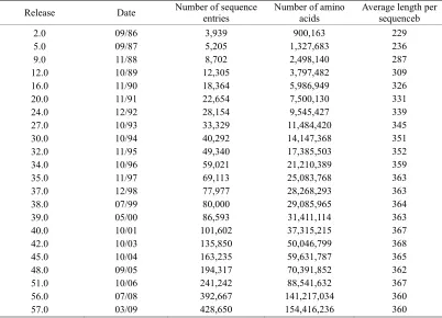
Table 1. The growth of protein sequences in SWISS-PROT data banka_.

Release Date Number of sequence_entries Number of amino_acids Average length per _sequenceb

2.0 5.0 9.0 12.0 16.0 20.0 24.0 27.0 30.0 32.0 34.0 35.0 37.0 38.0 39.0 40.0 42.0 45.0 48.0 51.0 56.0 57.0

09/86 09/87 11/88 10/89 11/90 11/91 12/92 10/93 10/94 11/95 10/96 11/97 12/98 07/99 05/00 10/01 10/03 10/04 09/05 10/06 07/08 03/09

3,939 5,205 8,702 12,305 18,364 22,654 28,154 33,329 40,292 49,340 59,021 69,113 77,977 80,000 86,593 101,602 135,850 163,235 194,317 241,242 392,667 428,650

900,163 1,327,683 2,498,140 3,797,482 5,986,949 7,500,130 9,545,427 11,484,420 14,147,368 17,385,503 21,210,389 25,083,768 28,268,293 29,085,965 31,411,114 37,315,215 50,046,799 59,631,787 70,391,852 88,541,632 141,217,034 154,416,236

229 236 287 309 326 331 339 345 351 352 359 363 363 364 363 367 368 365 362 367 360 360

a. From

b. The average length per sequence is defined as the total number of amino acids divided by the total number of sequences. The quotient is rounded to an integer.

2. WEB-SERVERS

Recently, a series of web-servers have been developed in our group, as described below.

2.1. Cell-PLoc

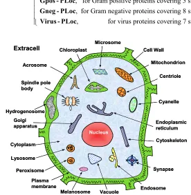
Thought by many as the most basic structural and func-tional unit of all living organisms, a cell is constituted by many different components, compartments or organelles (Figure 2), and they are specialized to perform different tasks. For instance: cytoplasm, a jelly-like material, takes up most of the cell volume, filling the cell and serving as a “molecular soup” in which all of the cell’s organelles are suspended; cell membrane functions as a boundary layer to contain the cytoplasm, while cell wall provides protection from physical injury; the cell nu-cleus contains the genetic material (DNA) governing all functions of the cell; the cytoskeleton functions as a cell’s scaffold, organizing and maintaining the cell’s shape, as well as anchoring organelles in place; mito-chondrion is the “power generator” playing a critical role

in generating energy in the eukaryotic cell; and so forth. However, most of these functions, which are critical to the cell’s survival, are performed by the proteins in a cell [4,5]. Divided by many different compartments or

or-ganelles usually termed as “subcellular locations”

(Fig-ure 2), a cell typically contains approximately one

bil-lion or ₁₀9 _{protein molecules each having its own}

lo-cation (for a single-lolo-cation protein) or lolo-cations (for a multiple-location or multiplex protein). Therefore, one of the fundamental goals in proteomics and cell biology is to identify the subcellular localization of proteins and their functions.

During the past 18 years, varieties of predictors have been developed to address this problem (see, e.g., [6-48] and the relevant references cited in a recent review paper [49].

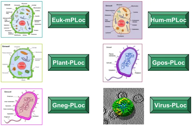
Developed recently, the Cell-PLoc [50] package

con-tains a set of six web-servers for predicting subcellular localization of proteins in six different organisms. The six web servers and their coverage scopes can be sum-marized by the following formulation

, for eukaryotic proteins covering 22 sites , for human proteins covering 14 sites , for plant proteins covering 11 sites , f



Euk - mPLoc Hum - mPLoc Plant - PLoc Cell - PLoc

Gpos - PLoc or Gram positive proteins covering 5 sites , for Gram negative proteins covering 8 sites , for virus proteins covering 7 sites

        

Gneg - PLoc Virus - PLoc

(1)

Nucleus

Plasma membrane Cytoplasm

Chloroplast Cell Wall

Mitochondrion

Endoplasmic reticulum

Cytoskeleton

Peroxisome Lysosome

Golgi apparatus

Centriole Extracell

Vacuole

Cyanelle

Hydrogenosome Spindle pole body

Endosome Synapse Microsome

Acrosome

Melanosome

Nucleus Nucleus

Plasma membrane Cytoplasm

Chloroplast Cell Wall

Mitochondrion

Endoplasmic reticulum

Cytoskeleton

Peroxisome Lysosome

Golgi apparatus

Centriole Extracell

Vacuole

Cyanelle

Hydrogenosome Spindle pole body

Endosome Synapse Microsome

Acrosome

Melanosome

K. C. Chou et al. / Natural Science 1 (2009) 63-92

where the character “m” in front of “PLoc” stands for “multiple”, meaning that the corresponding predictor can be used to deal with both single-location and multiple- location proteins.

To use the web-server package, just do the following

procedures. (1) Open the webpage

will see the top page of the Cell-PLoc package [50] on

your computer screen, as shown in Figure 3. (2) To

pre-dict the subcellular localization of eukaryotic proteins, click the “Euk-mPLoc” button; to predict the subcellular localization of human proteins, click the “Hum-mPLoc” button; to predict the subcellular localization of plant

proteins, click the “Plant-PLoc” button; and so forth. (3)

Now, you can follow the procedures (3) – (11) as de-scribed in [50] to get the desired results for the query proteins in the six different organisms.

To maximize the convenience for the people working in the relevant areas, each of the six predictors in the Cell-PLoc package has been used to identify all the pro-tein entries in the corresponding organism (except those annotated with “fragment” or those with less than 50 amino acids) in the Swiss-Prot database that do not have subcellular location annotations or are annotated with uncertain terms such as “probable”, “potential”, “likely”, or “by similarity”. These large-scale predicted results can be directly downloaded by clicking the Download button after getting on the top page of each of the six web-servers. These results can serve two purposes: one is that they can be directly used by those who need the information immediately; the other is to set a preceding mark to examine the accuracy of these web-server

pre-dictors by the future experimental results.

For example, listed in Appendix A are 334 eukaryotic

proteins. Their experimental annotated subcellular loca-tions were not available before Swiss-Prot 53.2 was re-leased on 26-June-2007. However, according to the large-

scale predicted results by Euk-mPLoc that were submitted

for publication on November-12-2006 as Supporting Infor-mation B in [51] and were also at the same time placed in

the downloadable file called Tab_Euk-mPLoc at

[50] or dicted subcellular locations of the 334 eukaryotic

pro-teins are given in column 4 of Appendix A, where for

facilitating comparison the corresponding experimental results available about seven months later are also listed in column 5. From the table we can see the following: of the 334 eukaryotic proteins, 309 are with single location site and 25 with multiple location sites. Of the 309 single location proteins, only 22 were incorrectly predicted; of the 25 multiple location proteins, 2 (i.e., No.104 and No.322) were incorrectly predicted. It is interesting to see that the predicted result for No.104 was “Centriole; Nucleus” while the experimental observation “Cyto-plasm; Nucleus”, meaning only one of its two location sites was incorrectly predicted; and that the predicted result for No.322 was “Centriole; Cytoplasm; Nucleus” while the experimental observation “Nucleus; Cyto-plasm”, meaning both of its observed location sites were correctly predicted although the site of “Centriole” was over-predicted. Accordingly, the overall success rate for the 334 proteins is over 93% as proved later by experi-ments.

Cell-PLoc: A package of web-servers for predicting subcellular localization of proteins in different organisms

Euk-mPLoc

Plant-PLoc

Gneg-PLoc

Hum-mPLoc

Gpos-PLoc

Virus-PLoc

Figure 3. A semi-screenshot to show the Cell-PLoc web-page at

Although the predictors in the Cell-PLoc package [50] are very powerful, they have the following shortcomings.

(1) In order for taking the advantage of Gene Ontology

(GO) [52] approach [49], the input for a query protein must include its accession number. However, many pro-teins, such as synthetic and hypothetical propro-teins, as well as those newly-discovered proteins that have not been deposited into databanks yet, do not have accession numbers, and hence their subcellular locations cannot be

predicted via the GO approach. (2) Since the current GO

database is far from complete yet, many proteins cannot be meaningfully formulated in a GO space even if their

accession numbers are available. (3) Although the

PseAA (pseudo amino acid) composition [18,53] or PseAAC approach, a complement to the GO approach in Cell-PLoc, can take into account some partial sequence order effects, the original PseAAC [18] missed the func-tional domain (FunD) [23] and sequential evolution (SeqE) information [54,55]. To improve the

aforemen-tioned shortcomings, the Cell-PLoc package is currently

under developing to be a new version, the Cell-PLoc 2.0.

At this stage, some of the predictors therein, such as Hum-mPLoc2.0[56], Plant-mPLoc [56], Gpos-mPLoc

[57], and Gneg-mPLoc [58], have been completed, as

will be briefed below.

To show the difference of Hum-mPLoc 2.0 with the

original Hum-mPLoc [44] in the Cell-PLoc package

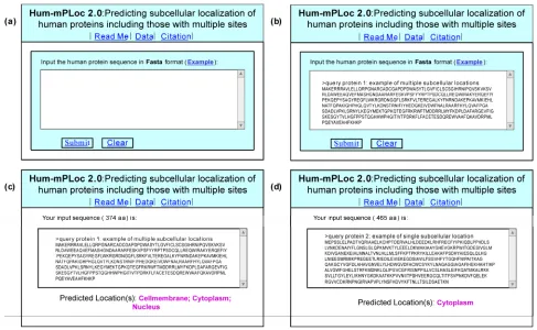
[55], let us see the following demonstration steps. Step1.Open the webpage

http://www.csbio.sjtu.edu.cn/bioinf/hum-multi-2/, and you will see its top page on your computer screen [50], as shown in Figure 4a.

Step 2. Either type or copy and past the query protein sequence into the input box (depicted by the box at the

center of Figure 4a). The input sequence should be in

FASTA format ( as shown by clicking on the Example button right above the input box. For example, if you use the 1st query pro-tein sequence in the Example window, the input screen should look like the illustration in Figure 4b.

Step 3. After clicking the Submit button, you will see “Cell membrane; Cytoplasm; Nucleus” shown on the screen (Figure 4c) after 15 seconds or so, indicating that the query protein is a multiplex protein that may simul-taneously exist in the three subcellular location sites, fully in agreement with experimental observations.

Step 4. If using the 2nd _{query protein sequence in the} Example window as an input, after clicking the Submit

K. C. Chou et al. / Natural Science 1 (2009) 63-92

button, you will see “Cytoplasm” shown on the screen

(Figure 4d), indicating the query protein is a sin-gle-location protein residing at the cytoplasm compart-ment or organelle, also fully in agreecompart-ment with experi-mental observations.

As we can see from the above steps, no accession numbers whatsoever are needed for the input data. This is quite different with the cases when using the original Hum-mPLoc in [55] to conduct prediction. Furthermore, the success rate expectancy has also been enhanced ow-ing to takow-ing into account the FunD and SeqE informa-tion.

Besides the improvements mentioned above, the

de-velopments from Plant-PLoc [43] in the Cell-PLoc

package [50] to Plant-mPLoc [59], from Gpos-PLoc

[60] to Gpos-mPLoc [57], and from Gneg-PLoc [61] to

Gneg-mPLoc [58], have made it possible to deal with the multiple-location problem for plant proteins, Gram- positive bacterial proteins, and Gram-negative bacterial proteins, respectively, as well.

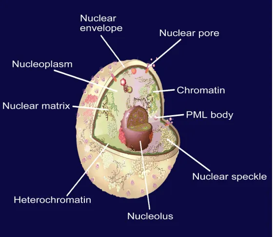
2.2. Nuc-PLoc

The nucleus exists only in eukaryotic cells. Located at the center of a cell like its kernel, the nucleus is the most prominent and largest cellular organelle [5], with the

diameter from 11 to 22 micrometers (μm) and occupying

about 10% of the total volume of a typical animal cell [62]. The life processes of a eukaryotic cell are guided by its nucleus. In addition to the genetic material, the

cellular nucleus contains many proteins located at its different compartments, called subnuclear locations. Therefore, the information of protein subnuclear local-ization is not only equally important to that of protein subcellular localization but also possesses the sense at a deeper level.

By fusing the SeqE approach and PseAAC approach

[63], a web-server called Nuc-PLoc was developed that

is accessible to the public via the website

. It can be used to identify nuclear proteins among the following nine subnuclear locations: (1) chromatin, (2) hetero-chromatin, (3) nuclear envelope, (4) nuclear matrix, (5) nuclear pore complex, (6) nuclear speckle, (7) nucleolus,

(8) nucleoplasm, (9) nuclear PML body (Figure 5).

2.3. Signal-CF

Functioning as a “zip code” or “address tag” in guiding proteins to the cellular locations where they are sup-posed to be (Figure 6), signal peptides control the entry of virtually all secretory proteins to the pathway, both in eukaryotes and prokaryotes [64-66]. If the signal peptide for a nascent protein was changed, the protein could end in a wrong cellular location causing a variety of strange diseases. Accordingly, knowledge of signal peptides can be utilized to reprogram cells in a desired way for future cell and gene therapy. However, to realize this, an indis-pensable thing is to identify the signal peptide for a

Nucleus

Plasma membrane

Cytoplasm

Mitochondria

Endoplasmic reticulum

Cytoskeleton

Peroxisome Lysosome

Golgi apparatus

Centriole

Extracell

Signal protein

Nucleus

Nucleus

Plasma membrane

Cytoplasm

Mitochondria

Endoplasmic reticulum

Cytoskeleton

Peroxisome Lysosome

Golgi apparatus

Centriole

Extracell

Signal protein

Figure 6. A schematic drawing to show: how the signal peptides of secretory proteins function as an “address tag” in directing the proteins to their proper cellular and extracellular locations. The signal peptide sequence is colored in puple, and the mature protein sequence in blue.

Signal Peptidase

-Ls

-4 -2

-1 +1

+2

+L_m

-3

Signal Peptidase

-Ls

-4 -2

-1 +1

+2

+L_m

-3

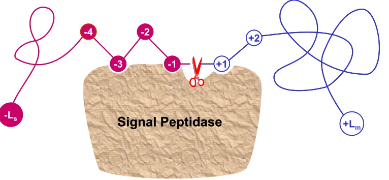
Figure 7. A schematic drawing to show the signal sequence of a protein and how it is cleaved by the signal peptidase. An amino acid in the signal part is depicted as a red circle with a white number to indicate its sequential position, while that in the mature protein depicted as an open circle with a blue number. The signal sequence contains Ls residues and the mature protein Lm residues. The cleavage site is at the position (-1, +1), i.e., between the last residue of the signal sequence and the first residue of the mature protein.

nascent protein. Many efforts have been made in this regards (see, e.g., [67-76] as well as the relevant refer-ences listed in a review article [77]).

K. C. Chou et al. / Natural Science 1 (2009) 63-92

a membrane (Figure 7), where the cleavage site is

commonly symbolized by ( 1, +1) , namely the

posi-tion between the last residue of the signal peptide and the first residue of the mature protein. It can also be seen

from Figure 7 that once the cleavage site is identified,

the corresponding signal peptide is automatically known; and vice versa.

The difficulty in predicting signal peptides is that for different secretory proteins, their signal peptides are quite different not only in sequence components and sequence orders but also in sequence lengths. Also, many previous methods were lacking of considering the coupling effects of the subsites around the cleavage sites, as analyzed in [78].

To address the above two problems, the web-server

predictor called Signal-CF [79] was developed recently.

Its features are reflected by its name, where “C” stands

for “Coupling” and “F” for “Fusion”, meaning that

Sig-nal-CF is formed by incorporating the subsite coupling effects along a protein sequence and by fusing the results derived from many width-different scaled windows through a voting system.

Signal-CF is a 2-layer predictor: the 1st_-layer predic-tion engine is to identify a query protein as secretory or

non-secretory; if it is secretory, the process will be auto-

matically continued with the 2nd_{-layer prediction engine}

to further identify the cleavage site of its signal peptide. The predictor is also featured by high success prediction rates with short computational time, and hence is par-ticularly useful for the analysis of large-scale datasets. Signal-CF is freely accessible at

. 2.4. Signal-3L

This is a 3-layer predictor developed for identifying the signal peptides of human, plant, animal, eukaryotic, Gram-positive, and Gram-negative proteins. The target of the 1st-layer is to identify a query protein as secretory or non-secretory. If the protein is identified as secretory, the process will be automatically continued by the 2nd- layer prediction engine to identify the potential cleavage

sites (Figure 7) along its sequence. The 3rd-layer is to

finally determine the unique cleavage site through a

global sequence alignment operation. Signal-3L is

ac-cessible to the public as a web-server at

http://chou.med.harvard.edu/bioinf/Signal-3L/. Compared

with Signal- CF, it might take a little longer

computa-tional time but yield a little higher accuracy.

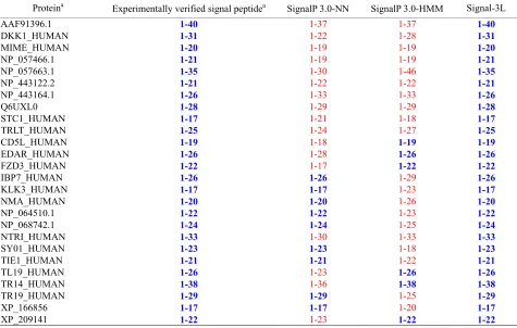
Table 2. List of examplesshowing that signal peptides miss-predicted by SignalP-NN and/or SignalP-HMM are corrected by Sig-nal-3L.

Proteina _{Experimentally verified signal peptide}a _{SignalP 3.0-NN SignalP 3.0-HMM Signal-3L}

AAF91396.1 1-40 1-37 1-37 1-40

DKK1_HUMAN 1-31 1-22 1-28 1-31

MIME_HUMAN 1-20 1-19 1-19 1-20

NP_057466.1 1-21 1-19 1-19 1-21

NP_057663.1 1-35 1-30 1-46 1-35

NP_443122.2 1-21 1-22 1-22 1-21

NP_443164.1 1-26 1-33 1-33 1-26

Q6UXL0 1-28 1-29 1-29 1-28

STC1_HUMAN 1-17 1-21 1-18 1-17

TRLT_HUMAN 1-25 1-24 1-27 1-25

CD5L_HUMAN 1-19 1-18 1-19 1-19

EDAR_HUMAN 1-26 1-28 1-26 1-26

FZD3_HUMAN 1-22 1-17 1-22 1-22

IBP7_HUMAN 1-26 1-26 1-29 1-26

KLK3_HUMAN 1-17 1-17 1-23 1-17

NMA_HUMAN 1-20 1-20 1-26 1-20

NP_064510.1 1-22 1-22 1-23 1-22

NP_068742.1 1-24 1-24 1-25 1-24

NTRI_HUMAN 1-33 1-30 1-33 1-33

SY01_HUMAN 1-23 1-23 1-18 1-23

TIE1_HUMAN 1-21 1-21 1-22 1-21

TL19_HUMAN 1-26 1-23 1-26 1-26

TR14_HUMAN 1-38 1-36 1-38 1-38

TR19_HUMAN 1-29 1-29 1-25 1-29

XP_166856 1-17 1-17 1-20 1-17

XP_209141 1-22 1-23 1-22 1-22

Both Signal-CF and Signal-3L can be used to refine the results by other predictors in this area. For instance, listed in Table 2 are the signal peptides that were miss-

predicted by SignalP-NN and/or SignalP-HMM in the

SignalP package [75] but corrected by Signal-3L. Also, according to a recent report (see Table 1 of [80]) Signal-CF performed the best in predicting the long signal peptides, among the following eight web-server

predictors: SignalP-NN [75], SignalP-HMM [75],

Sig-nalP-NN or SignalP-HMM [75], Phobius [81], PrediSi [76], Signal-CF [79], Signal-3L [82], and Philius [83]. 2.5. MemType-2L

Given a protein sequence, how can one identify whether it is a membrane protein or not? If it is, which membrane protein type it belongs to? It is important to address these problems because they are closely relevant to the biological function of the protein concerned and to its interaction process with other molecules in a biological system. Most functional units or organelles in a cell are “enveloped” by one or more membranes, which are the structural basis for many important biological functions. Although the basic structure of membranes is lipid bi-layer, many specific functions of the cell membrane are performed by the membrane proteins (see, e.g., [4,5]). For example, it is through membrane proteins that vari-ous chemical messages such as nerve impulses and hor-mone activity can be passed between cells (see, e.g., [84]); that cells can be attached to an extracellular matrix in grouping cells together to form tissues; that parts of the cytoskeleton can be attached to the cell membrane in order to provide shape; that the metabolism process and body’s defense mechanisms can be completed; as well as that molecules can be transported into and out of cells by such methods as proton pumps (see, e.g., [85-87]) and ion pumps (see, e.g., [88,89]), channel proteins [90-92] and carrier proteins (see, e.g., [93]).

Membrane proteins possess different types, which are closely correlated with their functions. For instance, the transmembrane proteins can transport molecules across the membrane or function on both its sides, whereas proteins functioning on only one side of the lipid bilayer are often associated exclusively with either the lipid monolayer or a protein domain on that side. Therefore, information about membrane protein type can provide useful hints for determining the function of an unchar-acterized membrane protein. Furthermore, because of the fluid nature of their infrastructure, membrane proteins can move around the cell membrane so as to reach where their function is required. Therefore, it will certainly expedite the pace in determining the function and action process of uncharacterized membrane proteins if we can timely acquire the knowledge of their type. With the

avalanche of protein sequences generated in the post genomic age and the fact that membrane proteins are encoded by 20-35% of genes [94], it is self-evident why it is so important to develop a sequence-based automated method for fast and effectively addressing the two prob-lems posed at the beginning of this Section.

Stimulated by the encouraging results in predicting the structural classification of proteins based on their amino acid (AA) composition or AAC [95-103], the co-variant discriminant algorithm was introduced to identify the types of membrane proteins also based on their AA composition in 1999 [104]. However, the AA composi-tion does not contain any sequence order informacomposi-tion. To avoid completely losing the sequence order information, the PseAA composition or PseAAC was introduced [18]. Since then, various prediction methods have been pro-posed in this area [53,105-118].

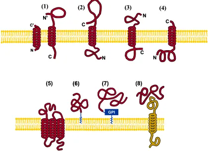
Recently, a user-friendly web-server predictor called “MemType-2L” was developed [54]. Compared with the other predictors which only cover 5-6 membrane

types, MemType-2L can cover 8 membrane types

(Fig-ure 8). MemType-2L is a 2-layer predictor: the 1st _layer prediction engine is to identify a query protein as mem-brane or non-memmem-brane; if it is memmem-brane, the process

will be automatically continued with the 2nd_-layer

pre-diction engine to further identify its type among the fol-lowing eight categories (Figure 8): (1) type I, (2) type II, (3) type III, (4) type IV, (5) multipass, (6) lipid-chain- anchored, (7) GPI-anchored, and (8) peripheral.

MemType-2L is accessible to the public via the

web-site at.

2.6. EzyPred

Nearly all known enzymes are proteins that catalyze chemical reactions and are vitally important in the me- tabolic process. Given a protein sequence, how can we identify whether it is an enzyme or non-enzyme? If it is, which main functional class it belongs to? What about its sub functional class? These problems are closely correlated with the biological function of an uncharac-terized protein and its acting object and process [119]. Although their answers can be found by conducting various biochemical experiments, it is both time-con-suming and costly to do so solely by experimental ap-proaches. During the last six years, a number of predic-tors have been developed to address these problems [53,120-125].

Recently, a top-down automated method called “Ezy-

Pred” was developed [126]. It not only covers all the six

K. C. Chou et al. / Natural Science 1 (2009) 63-92

C

N

(5)

(6)

(7)

GPI

(8)

N N'

C

C

N C

C'

N

(1)

₍₂₎

₍₃₎

₍₄₎

C

N

(5)

(6)

(6)

(7)

GPI

(7)

GPI

(8)

N N'

C

C

N C

C'

N

(1)

₍₂₎

₍₃₎

₍₄₎

Figure 8. Schematic illustration showing the 8 types of membrane proteins: (1) type I transmembrane, (2) type II, (3) type III, (4) type IV, (5) multipass transmembrane, (6) lipid-chain-anchored membrane, (7) GPI-anchored mem-brane, and (8) peripheral membrane. As shown in the figure, types I, II, III, and IV are all of single-pass transmem-brane proteins; see [253] for a detailed description about their difference. Reproduced from [54] with permission.

the 2nd _{layer for the main functional class; and the 3}rd

layer for the sub functional class. Within 90 seconds of submitting the sequence of a query protein into its input

box, EzyPred will identify whether the query protein is

enzyme or non-enzyme and, if it is an enzyme, to which main-functional class and sub-functional class it be-longs.

EzyPred is accessible to the public as a web-server at

2.7. ProtIdent

Called by many as the biology’s version of Swiss army knives, proteases cut long sequences of amino acids into fragments and regulate most physiological processes. They are vitally important in life cycle and have become a main target for drug design (see, e.g., [2,128-134]).

The actions of proteases are exquisitely selective (see, e.g. [135-139]), with each protease being responsible for splitting very specific sequences of amino acids under a preferred set of environmental conditions. According to their catalytic mechanisms, proteases are classified the following six types: (1) aspartic, (2) cysteine, (3)

glu-tamic, (4) metallo, (5) serine, and (6) threonine [140]. Different types of proteases have different action mechanisms and biological processes.

Therefore, it is important for both basic research and drug discovery to consider the following two problems. Given the sequence of a protein, can we identify whether it is a protease or non-protease? If it is, what protease type does it belong to?

During the last three years, some efforts have been made in this regard [141,142]. However, none of these methods provided a web-server that can be easily used by the majority of experimental and pharmaceutical sci-entists to obtain the desired data.

Very recently, a web-server called “ProtIdent” was

developed [55] by fusing the FunD (functional domain)

and SeqE (sequential evolution) information (Figure

10a). ProtIdent is a 2-layer predictor: the 1st layer is for identifying a query protein as protease or non-protease; if it is a protease, the process will automatically go to the second layer to further identify it among the six different mechanistic types (Figure 10b).

provided for demonstrating how to use the ProtIdent web-server, by which one can get the desired 2-level re-sults for a query protein sequence in around 25 seconds.

ProtIdent is freely accessible to the public via the site at .

2.8. GPCR-CA

One of the largest families in the human genome is the one encoding the G-protein-coupled receptors (GPCRs), which are cell surface receptors. Owing to their charac-teristic transmembrane topology, GPCRs are also known as 7-transmembrane receptors, 7TM receptors, hepta-helical receptors, and serpentine receptors that “snake”

K. C. Chou et al. / Natural Science 1 (2009) 63-92

Fusion

RPS-Blast

CDD

……

Generate FunD descriptor for P

Generate PsePSSM descriptor for P

……

1(1, μ)

1(1, μ)

 11(2, (2, μμ)) 11(10, (10, μμ)) 2(1,0,μ) 22(1,1,(1,1,μμ)) 22(10,49,(10,49,μμ))

Final protease type Input protein

sequence P

OET-KNN

Swiss-Prot

OET-KNN

PSI-Blast

a Base

Input a protein sequence

ProtIdent ensemble classifier

( = 2)

Protease

ProtIdent ensemble classifier

(= 6)

Non-protease

Stop

Final protease type Training

dataset I

Training dataset II

(a) (b)

Figure 10. A flowchart to show (a) how to fuse the FunD approach and PsePSSM approach, and (b) how the two-layer Prot-Ident ensemble classifier works in identifying proteases and their functional types. See [55] for further explanation.

Lipid

bilayer

2

2

3

3

4

4

5

5

1

1

₆

₆

7

7

Intracelluar

Extracellular

N

C

across a cell membrane seven times (Figure 11). The major role of GPCRs is to transmit signals into the cell. GPCR-associated proteins may play at least the follow-ing four distinct roles in receptor signalfollow-ing [144-147]: (1) directly mediate receptor signaling, as in the case of G proteins; (2) regulate receptor signaling through control-ling receptor localization and/or trafficking; (3) act as a scaffold, physically linking the receptor to various ef-fectors; (4) act as an allosteric modulator of receptor conformation, altering receptor pharmacology and/or other aspects of receptor function.

Much effort has been invested for studying GPCRs by both academic institutions and pharmaceutical in-dustries. Today, approximately one third of the world small molecule drug markets are GPCR agonists and antagonists.

The functions of many of GPCRs are still unknown, and it is both time-consuming and costly to determine their ligands and signaling pathways. Particularly, as membrane proteins, GPCRs are very difficult to crystal-lize and most of them will not dissolve in normal sol-vents. Accordingly, so far very few crystal GPCR struc-tures have been determined. Although the recently de-veloped state-of-the-art NMR technique is a very

pow-erful in determining the 3D structures of membrane pro-teins [87,92-94,148], it is time-consuming and costly. In order to timely obtain the protein 3D structures for ra-tional drug design, the approach of structural bioinfor-matics has been often adopted (see, e.g., [84,149-153]). Unfortunately, such an approach fails to work in most GPCR-related cases because very few GPCRs have suf-ficiently high sequence similarity with existing struc-ture-known proteins, an indispensable condition for de-veloping a reasonable starting structure via structural bioinformatics [2,3]. Consequently, it is highly desired to develop automated methods that can fast and effectively identify the functional families of GPCRs according to their sequence information because the information thus obtained can help classifying drugs, a technique called “evolutionary pharmacology” quite useful for drug de-velopment.

During the last 7 years or so, a number of methods were proposed in this regard [154-159]. Some of them were developed for identifying the main functional classes of GPCRs (see, e.g., [157]) and some for the sub- func-tional classes (see, e.g., [155]). None of these methods has provided a web-server for the public usage, and hence their practical application value is quite limited.

(a1)

(a2)

(b1)

(b2)

K. C. Chou et al. / Natural Science 1 (2009) 63-92

(a)

(b)

(c)

(d)

(e)

(f)

Figure 13. The cellular automaton image generated according to Eqs.2-5 for a protein taken from (a) A-rhodopsin like family, (b) B-secretin like family, (c) C-metabotrophic/glutamate/pheromone family; (d) D-fungal pheromone family, (e) E-cAMP receptor family, and (f) F-Frizzled/Smoothemed family, respectively. The six panels have completely dif-ferent textures because they represent six difdif-ferent GPCR family members.

Recently, a web-server predictor was developed [160]

with the name as GPCR-CA, where “CA” stands for

“Cellular Automaton” [161], meaning that the cellular automaton images have been utilized to reveal the pattern features hidden in piles of long and complicated protein sequences. Cellular automata are discrete dynamical sys-tems whose behavior is completely specified in terms of a local relation. A cellular automaton can be thought of as a stylized universe consisting of a regular grid of cells, each of which is in one of a finite number of possible states, updated synchronously in discrete time steps ac-cording to a local, identical interaction rule [162].

The procedures of generating the cellular automaton images for protein sequences can be briefed as follows. As a first step, each of the 20 native amino acids in a protein sequence is represented by a 5-digit strain ac-cording to the binary coding as defined in [163]. Thus, a

protein consisting of N amino acids can be converted

to a sequence with 5N digits (or grids); i.e,,

1 2 5

g ( )g ( ) g ( ) g ( ), (t t  _N t  _N t t0) (2) where g ( ) 0 or 1_i t  (i1, 2, , 5 )N as defined in [163]. Suppose the time for each updated step is con-secutively expressed by t0, 1, 2, , , we have

1 2 5

1 2 5

1 2 5

g (0) g (0) g (0) g (0)

g (1) g (1) g (1) g (1)

g (2) g (2) g (2) g (2)







 

 

 



N N

N N

N N

1 2 5

g ( )g ( ) g ( ) g ( ) 

          

 

    

  N  N

(3)

-1 1

-1 1

-1 1

-1 1

0, if g ( ) 0, g ( ) 0, g ( ) 0 0, if g ( ) 0, g ( ) 0, g ( ) 1 1, if g ( ) 0, g ( ) 1, g ( ) 0 0, if g ( ) 0, g ( ) 1, g ( ) 1

g ( 1)

1,                  

i i i

i i i

i i i

i i i

i

t t t

t t t

t t t

t t t

t

-1 1

-1 1

-1 1

-1 1

( 0, 1, , ) if g ( ) 1, g ( ) 0, g ( ) 0

0, if g ( ) 1, g ( ) 0, g ( ) 1 1, if g ( ) 1, g ( ) 1, g ( ) 0 0, if g ( ) 1, g ( ) 1, g ( ) 1

          _{ }  _{  }   _{  }       _{  }  

i i i

i i i

i i i

i i i

t

t t t

t t t

t t t

t t t

(4)

with the spatially periodic boundary conditions; i.e.,

0 5

g ( ) g ( )t  _N t and g_5N1( ) g ( )t  ₁ t (5) Suppose: g ( )_i t , the thi grid at t, is filled with white color if g ( ) 0_i t  and black if g ( ) 1_i t  .

Accord-ingly, each row of Eq.3 corresponds to a narrow ribbon

mixed with white and black colors. Scanning these rib-bons successively on to a screen or sheet will generate a 2D (2-dimensional) black-and-white image. It has been observed that the image texture is basically steady after

100

  

t . The image thus evolved is called the

cellu-lar automaton image for the protein sequence concerned. The advantage of using the cellular automaton image to represent the protein is that it can help us visualize some special features hidden in its long and complex sequence [163]. For instance, the cellular automata images for proteins from a same GPCR family share a similar textu-

re pattern (Figure 12), while those from different GPCR

families have different texture patterns (Figure 13). Subsequently, the gray-level co-occurrence matrix factors extracted from the cellular automaton images were used to represent the samples of proteins through their pseudo amino acid composition [18,53], followed by utilizing the augmented covariant-discriminant

clas-sifier [12,164] to operate the prediction of GPCR-CA.

GPCR-CA is a 2-layer predictor: the 1st layer predic-tion engine is for identifying a query protein as GPCR on non-GPCR; if it is a GPCR protein, the process will be automatically continued with the 2nd-layer prediction engine to further identify its type among the following six functional classes: (1) rhodopsin-like, (2) secretin- like, (3) metabotrophic/glutamate/pheromone; (4) fungal pheromone, (5) cAMP receptor, and (6) Frizzled/Smoo-

themed family. GPCR-CA is freely accessible at

, by which one can get the desired 2-layer results for a query protein sequence within about 20 seconds.

2.9. HIVcleave

During the past 17 years, the following two strategies have often been utilized to find drugs against AIDS (ac-quired immunodeficiency syndrome). One is to target

the HIV (human immunodeficiency virus) reverse tran-scriptase (see, e.g., [165-171]); the other is to design HIV protease inhibitors [128,136,138,139,172-174].

Functioning as a dimer, the HIV protease is made up of two identical subunits, each having 99 residues, but with only one active site [136,174]. The essential func-tion of HIV protease is to cleave the precursor polypro-tens; loss of the cleavage-ability will stop the life cycle of infectious HIV, the culprit [175,176] of AIDS. To find the effective inhibitors against HIV protease, it is very helpful to understand the mechanism of how it cleaves the polyproteins and utilize the “distorted key” theory [136] to approach the problem, as illustrated be-low. HIV protease is a member of the aspartyl proteases that is highly substrate-selective and cleavage-specific. The HIV protease-susceptible sites in a given protein extend to an octapeptide region [177], with its amino acid residues sequentially symbolized by eight subsites R₄ , R₃, R₂, R₁, R_1', R_2', R_3', R_4'

[178], as shown in Figure 14. The scissile bond is

lo-cated between the subsites R₁ and R_1'. Occasionally,

K. C. Chou et al. / Natural Science 1 (2009) 63-92

HIV Protease

R

R

R

R

R

R

R

R

N H H N N H H N C || O O || C C || O O || C H N H N N H N H O || C C || O C || O O || C

S

_S

2

S

S

S

S

S

S

HIV Protease

R

R

R

R

R

R

R

R

N H H N N H H N C || O O || C C || O O || C H N H N N H N H O || C C || O C || O O || C

S

_S

2

S

S

S

S

S

S

Figure 14. Schematic representation of substrate bound to HIV protease based an analysis of protease-inhibitor crystal struc-tures. The active site of enzyme is composed of eight extended “subsites”, S4, S3, S2, S1, S1’, S2’, S3’, S4’, and their counterparts in a substrate extend to an octapeptide region, sequentially symbolized by R4, R3, R2, R1, R1’, R1’, R2’, R3’, R4’, respectively. The scissile bond is located between the subsites R1 and R1’. Reproduced with permission from Figure 3 of K.C. Chou [136].

(a)

R1’

R2’

R3’

R4’

R1

R2

R3

R4

HIV Protease

R2’

R3’

R4’

R1 R2 R3 R4

HIV Protease

R1’

R2’

R3’

R4’

R1

R2

R3

R4

HIV Protease

R2’

R3’

R4’

R1

R2

R3

R4

HIV Protease

Figure 15. Schematic illustration to show (a) a cleavable oc-tapeptide is chemically effectively bound to the active site of HIV protease, and (b) although still bound to the active site, the peptide has lost its cleavability after its scissile bond is modified from a hybrid peptide bond [254] to a single bond by some simple routine procedure. The eight residues of the pep-tide is sequentially symbolized R4, R3, R2, R1, R1’, R1’, R2’, R3’, R4’. The scissile bond is located between R1 and R1’. Adapted from [136] with permission.

still bind to the active site of an enzyme. Actually, the molecule thus modified can be deemed as a “distorted key”, which can be inserted into a lock but can neither open the lock nor be pulled out from it. That is why a molecule modified from a cleavable peptide can sponta-neously become a competitive inhibitor against the en-zyme. An illustration about such a concept is given in Figure 15, where panel (a) shows an effective binding of a cleavable peptide to the active site of HIV protease,

while panel (b) shows that the peptide has become a

non-cleavable one after its scissile bond is modified al-though it can still tightly bind to the active site. Such a modified peptide, or “distorted key”, will automatically become an inhibitor candidate of HIV protease. Even for non-peptide inhibitors, it can also provide useful insights about the key binding groups, hydrophobic or hydro-philic environment, fitting conformation, et al. Accord-ingly, in search for the potential inhibitors, a matter of paramount importance is to discern what kind of pep-tides can be cleaved by HIV protease and what kind cannot be. Even if limited in the range of an octapeptide, it is by no means easy to address the question. This is because the number of possible octapeptides formed from 20 amino acids runs into ₂₀8_108log20_{2.56 10} 10_.

the pace in search for the proper inhibitors of HIV pro-tease would be significantly expedited. Actually, during the last decade or so, various prediction methods have been developed in this regard [128,135,137-139,180- 186].

Recently, based on the discriminant function

algo-rithm [136], a web server called HIVcleave [187] was

established at the website

protein sequence, one can use HIVcleave to predict its

cleavage sites by HIV-1 and HIV-2 proteases, respec-tively.

2.10. QuatIdent

As the chief actors of various biological processes in a cell, proteins have the following four different structural levels: primary, secondary, tertiary, and quaternary [188]. The primary structure refers to the constituent amino acid sequence; the secondary, to the local spatial ar-rangement of a polypeptide’s backbone without regard to the conformations of its side chains; the tertiary, to the three-dimensional structure of an entire polypeptide; and the quaternary, to how many polypeptide chains (sub-units) involved in forming a protein and the spatial ar-rangement of its subunits. The concept of quaternary structure is derived from the fact that many proteins are composed of two or more subunits which associate with each other through non-covalent interactions and, in some cases, disulfide bonds. According to the number of subunits aggregated together in an oligomeric complex, protein quaternary structures can be classified into: monomer, dimer, trimer, tetramer, pentamer, and so forth [189]. A statistical distribution of different quaternary

structural types is shown in Figure 16, from which we

can see that the nature prefers those oligomers with even and/or small number of subunits, fully consistent with the findings by the previous investigators [190,191]. If the subunits in a complex are identical, then the complex is called homo-oligomer; otherwise hetero-oligomer. For example, the sodium channel is formed by a monomer [192] while the potassium channel by a homo-tetramer [88]; the phospholamban is formed by homo-pentamer [93,193] while the Gamma-aminobutyric acid type A (GABAA) receptor by a hetero-pentamer [84,194]; the M2 proton channel is formed by a homo-tetramer [87] while hemoglobin by a hetero-tetramer [195].

Facing the explosion of newly generated protein se-quences, we are challenged to develop an automated method for rapidly and reliably identify the quaternary structural attributes of uncharacterized proteins because they are closely relevant to the functions and mecha-nisms of proteins (see, e.g., [87,195]. Besides, the in-formation thus obtained is very useful in screening the candidates of proteins for their 3D structure determina-tion. It is known that many functionally important

pro-teins exist in vivo as oligomers rather than single indi-vidual chains. For example, hemoglobin is a hetero-

tetramer of two α chains and two β chains, and the

four chains must be aggregated into one construct to perform its cooperative function during the oxygen- transporting process [195]. Also, the novel allosteric drug-inhibition mechanism for the M2 proton channel was recently revealed by the NMR observations [87,92]. It has been found through an in-depth analysis that such a subtle mechanism is closely correlated with a unique packing arrangement of four transmembrane helices from four identical protein chains [90,91,196]. For this kind of proteins, determination of their individual chains independently would be less interesting or should be avoided. Therefore, developing an effective method to predict the quaternary structural attributes of proteins based on their sequence information alone would pro-vide useful clues for both basic research and drug de-velopment.

To address the challenge, the web-server predictor

called “QuatIdent” [197] was developed recently by

fusing the functional domain and sequential evolution

information. QuatIdent is a 2-layer predictor. The 1st

layer is for identifying a query protein as belonging to which one of the following ten main quaternary struc-tural attributes: (1) monomer, (2) dimer, (3) trimer, (4) tetramer, (5) pentamer, (6) hexamer, (7) heptamer, (8) octamer, (9) decamer, and (10) dodecamer. If the result thus obtained turns out to be anything but monomer, the process will be automatically continued to further iden-tify it belonging to a homo-oligomer or hetero-oligomer. QuatIdent is freely accessible to the public as a web server via the site at

ch one can get the desired 2-level results for a query protein sequence in around 25 seconds. And the longer the sequence is, the more time that is needed.

2.11. PQSA-Pred

This is another web-server predictor [198] developed by hybridizing the functional domain composition approach and pseudo amino acid composition approach for pre-dicting protein quaternary structural attribute based on

the sequence information alone. PQSA-Pred can be

used to predict a query protein among the following three quaternary attributes according to its sequence in-formation: monomer, homo-oligomer, and heterooligo- mer. As a useful tool for crystallographic scientists in

screening for their targets, PQSA-Pred is freely

accessi-ble to the public via the website at

.

K. C. Chou et al. / Natural Science 1 (2009) 63-92

Monomer

14%

Dimer 50%

Trimer

6%

Tetramer

21%

Pentamer

_2%

Heptamer

5%

0.2%

Octamer 1%

Decamer 0.2%

0.3%

0.3%

Dodecamer

Others

Hexamer

Monomer

14%

Dimer 50%

Trimer

6%

Tetramer

21%

Pentamer

_2%

Heptamer

5%

0.2%

Octamer 1%

Decamer 0.2%

0.3%

0.3%

Dodecamer

Others

Hexamer

Figure 16. A pie chart to show the statistical distribution of different quaternary structural types in the nature derived from version 55.3 of Swiss-Prot database released 29-April-2008. Reproduced with permission from [197].

2.12. PFP-Pred

A protein can function properly only if it is folded into a very special and individual shape or conformation, i.e., has the correct secondary, tertiary and quaternary struc-ture [201]. Failure to fold into the intended 3D strucstruc-ture usually produces inactive proteins or misfolded proteins [202] that may cause cell death and tissue damage [203] and be implicated in prion diseases such as bovine spongiform encephalopathy (BSE, also known as “mad cow disease”) in cattle and Creutzfeldt-Jakob disease (CJD) in humans. All prion diseases are currently un-treatable and are always fatal [204].

Although the X-ray crystallography is a powerful tool in determining protein 3D structures, it usually takes months or even years to determine the structure of a sin-gle protein. Also, the determination might fail for those proteins (particularly membrane proteins) that are diffi-cult to crystallize. Although the nuclear magnetic reso-nance (NMR) technique is very powerful in determining membrane protein structures [87,93,94,148], it requires expensive equipments and take equally long or even longer time. The avalanche of protein sequences gener-ated in the Post Genomic Age has challenged us for de-veloping computational methods by which the structural information can be timely extracted from sequence da-tabases. Although the direct prediction of the 3D struc-ture of a protein from its sequence based on the least free energy principle [201,205] is scientifically quite sound

and some encouraging results already obtained in eluci-dating the handedness problems and packing arrange-ments in proteins (see, e.g., [206-211]), it is far from successful yet for predicting its 3D structure owing to the notorious local minimum problem except for some very special cases or by utilizing some additional infor-mation from experiments (see, e.g., [212,213]). Actually, it is even not successful yet for simply predicting the overall fold of a query protein based on its sequence alone. For further information about protein folding, refer to a recent review [214] and the references cited therein. Again, although it is quite successful to predict the 3D structure of a protein according to the homology modeling approach [2,215] as reflected by a series of homology-modeled proteins for drug development [84,147,149-151,153,216-226], a hurdle exists when the query protein does not have any structure-known ho-mologous protein in the existing databases [3].

Facing this kind of situation, a different strategy, the so-called taxonomic approach [227] was developed to address the problem. According to such a strategy, pre-dicting the 3D structure of a protein may be first con-verted to a problem of classification; i.e., identifying which fold pattern it belongs to. Its underpinning is based on the assumption that the number of protein folds is limited [228-231].

PFP-Pred [232] is one of these kinds of predictors. It was formed by a set of basic classifiers, with each trained in different parameter systems, such as predicted secondary structure, hydrophobicity, van der Waals vol- ume, polarity, polarizability, as well as different dimen-sions of pseudo amino acid composition, that were ex-tracted from a training dataset. The operation engine for the constituent individual classifiers was OET-KNN (Optimized Evidence-Theoretic K-Nearest Neighbors) rule [32,113,233]. Their outcomes were combined thru a weighted voting to give a final determination for classi-fying a query protein. The recognition was to find the true fold among the 27 possible patterns. The web-server of PFP-Pred is available to the public via the site

2.13. PFP-FunDSeqE

This is an improved version of PFP-Pred by combining

the functional domain information and the sequential evolution information through a fusion ensemble classi-fier [234], as reflected by parts of its name where “FunD” stands for “functional domain” while “SeqE” for “sequential evolution”. Compared with the other ex-isting methods for predicting the protein fold patterns, PFP-FunDSeqE can usually yield better results [234]. Its web-server is available at

2.14. Pred-PFR

Since each protein begins as a polypeptide translated from a sequence of mRNA as a linear chain of amino acids, it is interesting to study the folding rates of pro-teins from their primary sequences. Actually, protein chains can fold into the functional 3D structures with quite different rates, varying from several microseconds [235] to even an hour [236]. Since the 3D structure of a protein is determined by its primary sequence, we can assume the same is true for its folding rate. In view of this, we are challenged by an interesting question: Given a protein sequence, can we find its folding rate? Al-though the answer can be found by conducting various biochemical experiments, doing so is both time- con-suming and expensive. Also, although a number of pre-diction methods were proposed [237-242], they need the input from the 3D structure of the protein concerned, and hence the prediction is feasible only after its 3D struc-ture has been determined. However, according to data released on5-May-2009 by the RCSB Protein Data Bank ), the number of proteins with 3D structure known is only about 1.34% of the number of sequence-known proteins. Therefore, it is highly de-sired to develop an automated method that can rapidly

and approximately predict the folding rates of proteins according to their sequence information alone. Some ef-forts have been made in this regard (see, e.g., [243,244]).

Since the experimentally observed folding rate for a protein chain usually represents the “apparent folding rate constant” [245] as denoted by K_f, it is instructive to unravel its relationship with the detailed rate constants, as given below.

The apparent folding rate constant K_f for a protein

chain is defined via the following differential equation

unfold

f unfold fold

f unfold

dP ( )

P ( ) d

dP ( )

P ( ) d

t

K t

t t

K t

t

 _{ }

 

 _



(6)

where P_unfold( )t and P ( )_fold t represent the concentra-tions of its unfolded state and folded state, respectively.

Suppose the total protein concentration is C₀, and

ini-tially only the unfolded protein is present; i.e.,

unfold 0

P ( )t C and P ( ) 0fold t  when t0 .

Subse-quently, the protein system is subjected to a sudden change in temperature, solvent, or any other factor that causes the protein to fold. Obviously, the solution for Eq.6 is









unfold 0 f fold 0 f

P ( ) exp P ( ) 1 exp

t C K t

t C K t

  



 _{    }

  

 (7)

It can be seen from the above equation that the larger the

f

K , the faster the folding rate will be. Given the value of

f

K , the half-life of an unfolded protein chain can be

expressed by





1/ 2 f

f

ln 1/ 2

0.693

T K

K

   (8)

which can also be used to reflect the time that is needed for a protein chain to be half folded. However, the actual folding process is much more complicated than the one

as described by Eq.6 even if the reverse rate for the

folding system concerned can be ignored. As an illustra-tion, let us consider the following three-state folding mechanism

23 12

unfold inter fold

P k P k P (9)

where P_inter( )t represents the concentration of an in-termediate state between the unfolded and folded states,

12

K. C. Chou et al. / Natural Science 1 (2009) 63-92

unfold

12 unfold inter

12 unfold 23 inter fold

23 inter

dP ( )

P ( ) d

dP ( )

P ( ) P ( ) d

dP ( )

P ( ) d

t

k t

t t

k t k t

t t k t t  _{ }    _{ }      (10)

To get the solution of Eq.10, let us use an intuitive

dia-gram called “directed graph” or “digraph”  (Figure

17a) [245,246] to represent Eq.9. To reflect the variation of the concentrations of the three protein states with time,

the digraph  is further transformed to the phase

di-graph  [245,246] as shown in Figure 17b, where

s

is an interim parameter associated with the Laplace

transform as shown in Eq.11

.

 

 

 

unfold ₀ unfold inter ₀ inter

fold ₀ fold

P ( ) P ( ) exp d

P ( ) P ( ) exp d

P ( ) P ( ) exp d

s t ts t

s t ts t

s t ts t

    _{ }        _{ } 







where P_unfold, P_inter and P_fold are the phase concentra-tions of Punfold, Pinter and Pfold, respectively. Thus,

ac-cording to the phase digraph  of Figure 17b and using the graphic rule 4 [245,246], which is also called the graphic rule for non-steady-state kinetics” in litera-tures (see, e.g., [247]), we can directly write out the fol-lowing phase concentrations:



















unfold

12 23 12 23 12 12 23

P ( )s s k sC s k C C

s k s k s k s s k s k s k k

              

 _(12.1)











inter

12 23 23 12 12 23

P ( )s k s C k C

s k s k s s k s k s k k

 

 

  

 

 

 _(12.2)











fold

12 23 23 12 12 23

P ( )s k k C k k C

s s k s k s s k s k s k k

 

 

  

 

 

 _(12.3)

Through the above phase concentrations and using Laplace transform table (see, e.g., [248] or any standard mathematical tables), we can immediately obtain the desired concentrations for P_unfold, P_inter and P_fold of Eq.10, as given by Eq.13

.

unfold 0 12 0 inter

23 12 0

fold 12 23 0

23 12

12

23 12

23 12

P ( ) e

P ( ) e e

P ( ) e e

t C k C t

k k C

t k k C

k k

k t

k t k t

k t k t

 _   _{ }   _  _         _{  }    _{  }       (13)

Accordingly, it follows from Eq.13 that

23 12 fold 12 23 0 12 23 12 23

unfold 23 12 23 12

dP ( )

e e 1 e P

d

k t k k C t t k k

t k k k k

k t

k

k  _ _

   

 

 _   _   

   _ _

(14)

Comparing Eq.14 with Eq.6, we obtain the following equivalent relation

23 12 12 23

f

23 12

1 e k

k k K k k k t              

 _{ } (15) (a) (b)

unfold

P

P

12

k

P

k

P

P

12

k

P

k

P P_inter

12

k

k

s

s

s

unfold

P P_inter

12

k

k

s

s

s