Multivariate Bayesian forecasting models

University of Warwick institutional repository: http://go.warwick.ac.uk/wrap

A Thesis Submitted for the Degree of PhD at the University of Warwick

http://go.warwick.ac.uk/wrap/34805

This thesis is made available online and is protected by original copyright.

Please scroll down to view the document itself.

MULTIVARIATFO3AYESIAN

FORECASTING MODELS

JOSE MARIO QUINTANA

Thesis submitted for the degree of Doctor of Philosophy

DEPARTMENT OF STATISTICS UNIVERSITY OF WARWICK

MARCH 1987

CONTENTS

Summary

vii

CHAPTER 1. INTRODUCTION

1.1 Multivariate Forecasting Models 1 1.2 The Bayesian Approach 2

1.3 Tractability 3

1.4 Outline of the Thesis 4 1.5 Notation 6

CHAPTER2. THE DYNAMIC LINEAR MODEL

2.1 Model Formulation 7 2.2 Update Computations 8 2.3 Standard Models 9 2.4 Multivariate Models 11

2.5 Specification of the Variances 11 Appendix

A2.1 Polynomial Transition

Matrix 14

CHAPTER 3. DYNAMIC LINEAR MATRIX-VARIATE REGRESSION

3.1 Model Formulation 15 3.2 Update Computations 18 3.3 The DLMR as a DLM 20 3.4 Multi-process Models 23 3.5 Reparameterization 27 3.6 System Decoupling 28

3.7 Dynamic Weighted Multivariate Regression 29

Appendix A3.1 Kronecker Product and vec Operator 32

Appendix A3.2 Basic Matrix-variate Distribution Theory 35

CHAPTER 4. IMPLEMENTATION ASPECTS

4.1 Implementation via State-space Filters 43

4.2 Implementation via the Sweep Operator 46

CHAPTER 5. PLUG-IN ESTIMATION, INFORMATION AND

DYNAMIC LINEAR MODELS

5.1 Dynamic Linear Models 56

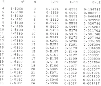
5.2 Example: Energy Consumption by Primary Fuel Inputs 62

Appendix A5.1 Plug-in Estimation and Information

74

Appendix A5.2 Entropy and Information of Useful Matrix-variate Distributions

79

CHAPTER 6. DYNAMIC RECURSWE MODEL AND DYNAMIC SCALE VARIANCE

6.1

Dynamic Recursive Model 81

6.2 Example: Hierarchical Missing Observations 85 6.3 Dynamic Scale Variance 88

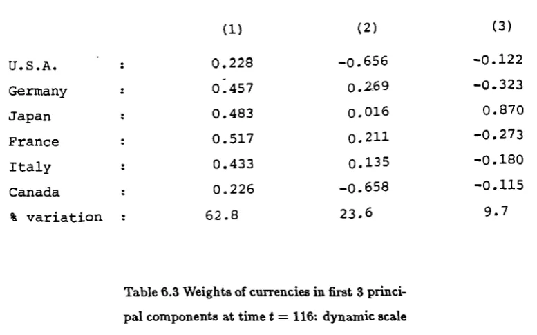
6.4 Example: Exchange Rate Dynamics 91

Appendix A6.1 Simulation

104

Appendix A6.2 Distribution of Swept Matrices

106

CHAPTER 7. MODELLING ASPECTS

7.1 Vague Priors 108 7.2 Transformations 108 7.3 Special Models 110

CHAPTER 8. DISCUSSION AND FURTHER RESEARCH

113

W

ACKNO4LEDGEMENTS

I would like to express my gratitudeto my supervisor Mike West. His excellent guidance, encour-agement and friendship made these years of research a very pleasant experience. Also, I am grateful to my fellow students and the members of the staff. In particular, Jo Crosse made my relationship with AS-TEX a lot easier, discussions and lessons with Jeff Harrison were illuminating, Tony O'Hagan kindly offered me a copy of his useful personal notes on matrix-variate distributions and pointed out many mistakes in an earlier version. Special thanks to Federico O'Reilly; he not only encouraged me to take these steps, but to a great extent made it possible. My wife Carol in a recent conversation with her mother said "..• and soon we will submit the thesis." If anything, she was being modest.

The astrologer and sorcerer-fortuneteller brought out the Book of the Horoscope, together with the calendar.

SUMMARY

This thesis concerns theoretical and practical Bayesian modelling of multivariate time series. Our main goal is to intruduce useful, flexible and tractable multivariate forecasting models and provide the necessary theory for their practical implementation.

CHAPTER 1 INTRODUCTION

The use of conditional probability as the basis for statistical analysis can be traced back to the work of Bayes (1763) in the eighteenth century. At the beginning of the following century Legendre and

Gauss published the method of linear least-squares that they developed working independently of each

other (Plackett, 1972). In this century, after a dark period, there has been a revival of Bayesian ideas

lead by de Finetti and others (Houle, 1983). Meanwhile, Plackett (1950) obtained a recursive solution

for linear least-squares, and Kalman and others (circa 1960) using state-space formulations designed

optimal recursive filters for the estimation of multivariate stochastic dynamic linear systems (Gelb,

1974). It soon became apparent that the Bayesian approach provided a neat theoretical framework for

the recursive estimation and control of stochastic systems (Ho and Lee, 1964; Aoki, 1967). The merits of

this kind of approach for time series and forecasting were evident with the introduction of the Dynamic

Linear Model of Harrison and Stevens (1976). This reformulation of the state-space models furnished a

time invariant interpretation of the system parameters, model building from simple components,

multi-process models, intervention analysis, etc.; a milestone that has stimulated a line of research leading to

a methodology known as Bayesian forecasting. This is the base upon which we build our multivariate Bayesian forecasting models.

1.1 MULTIVARIATE FORECASTING MODELS.

We are concerned with Bayesian multivariate forecasting models. First, we wish to stress what we

mean by a model. It is often assumed that there is a true underlying model, a set of fundamental "laws", which generates the observations in the real world and our task is to discover it. However,

it has been argued that no model used in practice is perfect (Maybeck, 1979, 1982a). Furthermore,

the uniqueness and even the existence of a true model will always be open to question (Dickey, 1976;

Dawid, 1986). Therefore, instead of searching for a utopia, we adopt a pragmatic approach in line with

Harrison and Stevens (1976): a model represents the way in which the observer looks at the observations

and their context. In addition, the models entertained are probabilistic, dynamic and Bayesian. The

observer does not have a procedure for predicting with perfect accuracy the following observations, and

the structure of the model itself is changing in an uncertain way as time passes. Thus, uncertainty is

incorporated in the observer's model, the observer is always open-minded and changes his/her mind by

means of Bayes' theorem as new information becomes available.

Multivariate forecasting models deal simultaneously with several univariate time series denoted by

The essential reason for considering joint multivariate time series as opposed to several marginal time

series is that, apart from a trivial case, the marginal predictive distributions do not provide enough

information in order to produce a proper joint predictive distribution. Furthermore, the

contemporane-ous joint variation of the observations is originally uncertain and a main goal of the time series analysis

is to learn about it. In so doing, the solution of practical decision problems, which depends on the joint

variation, is possible. Moreover, the joint predictive distribution provides a means of updating the

pre-dictive distribution of a subset of observations when another subset of contemporaneous observations is

given, or more generally, when information regarding another subset of contemporaneous observations

is given. Thus, the forecasting performance for univariate time series may be improved by looking at

them together with several related time series.

1.2 THE BAYESIAN APPROACH.

The models considered in this dissertation are Bayesian. Although the use of the Bayesian paradigm

in statistics is still somewhat controversial, our approach is justified if only for its simplicity. Instead

of working with an endless list of ad hoc non-Bayesian procedures, in Bayesian inference we only need

to make use of formal golden rules of probability for learning, prediction, etc.

The analysis of Bayesian dynamic models is in principle essentially as neat as the usual static Bayesian

analysis. Let y be a set (scalar, vector or matrix) of observations and 9 be a set (scalar, vector or matrix)

of parameters. The standard static model is defined by the observational density conditional on the

parameters (likelihood) p(y10) and the prior density p(0), then the predictive density p(y) and the

posterior density p(Oly) are obtained by means of the conglomerative property and Bayes' theorem,

p(y) = f _{p(y10) p(0) de and p (9}

₁

_{y) — P(YI °) PP) .} (1.1)

e PM

A lucid and brief exposition of the basic principles can be found in Zellner (1971, Chapter 2).

In a dynamic model the observational density conditional on the set of parameters, also called the

system state, is P(Yt l et)) where the state Ot is changing as time passes. The evolutional density which describes a Markovian transition from the state (4_ 1 to Ot is p(Ot lOt _ i ) and the prior information about

Elt _ i is represented by p(Ot _ 1 ). It is also implicitly assumed that these densities are conditional on the

history of the series up to time t — 1; see Section 1.5.

It is evident that a dynamic model can accommodate easily a static model. Conversely, a dynamic

model can be thought of as static at time t by taking y = yt, 0 =

(etIN) =

(et

is

, et-tbP0(11 0). = P(Yt let) fi

, P(9) =

P (et l e t-1) p(Ot _ 1). The cycle can be repeated as often as necessary since the next prior for t , in given

(t, et-liY) d

the past and present information, given by p _{-r-1 P e}

1

In summary, the et

dynamic model can be seen as static by considering jointly the parameters Ot and Ot _ i . Their joint

prior information is expressed in terms of the evolutional information and the prior information about

Ot _ i . The set of parameters Os_ i do not appear in the observational density for yt , but this is irrelevant

to the analysis. This representation is employed in Chapter 3 in order to formulate a general multivariate

dynamic linear model.

(1.2a)

(1.2b) A major criticism of the Bayesian viewpoint has been its lack of objectivity (misleadingly associated with the prior information). Nevertheless, there is no point in arguing about whether or not the non-Bayesian approaches are objective, since the meaning of objectivity itself is, in our opinion, very subjective! Instead of wasting more space discussing the Bayesian - non-Bayesian controversy, we refer the reader to the extensive literature on this recurrent topic: Berger (1985), Barnett (1982), de Finetti (1974, 1975), Lindley (1971), Dempster (1969), etc.

1.3 TRACTABILITY.

It is easy to see that, in the seemingly static representation, the key calculations needed for a dynamic model are simply:

POO = f P(Otl Ot- 1) P(Ot-1) dOt-i, et-1

P(Yt) = i P (Yt l et) get) det, and et

P(Yt l ilt) P(9t)

P( OtlYt) = (1.2c)

P(%) •

Equation (1.2a) gives the density of 0 at time t in terms of the evolutional density and the previous density of 0 at time t - 1 and represents our knowledge of 0 at time t before observing yt . The one-step ahead predictive density is provided by (1.2b). Finally, (1.2c) closes the cycle since it is the formula for updating the density' of Ot after observing yt . Long-term forecasting is achieved by applying (1.2a) and (1.2b) repeatedly, but, of course, skipping the updating formula (1.2c).

Successful implementation of equations (1.2) depends on the difficulties encountered in solving the integrals appearing in (1.2a) and (1.2b). Perhaps a not so obvious and even more critical factor

as pointed out by Aoki (1967, Appendix 4), is the existence of a tractable sufficient statistic of fixed

dimension for G. If such a tractable statistic exists then the complexity of the density of O t does not grow as time passes, and so is updated easily. A statistic is simply a function of the observations and a sufficient statistic for a set of parameters, by definition, summarizes all the. iuLarmation that the observations provide about the parameters. In other words, the distribution of the parameters conditioning on the observations is the same as the distribution obtained by conditioning only on the sufficient statistic. By a tractable statistic we mean a function of the observations which is easily computated. A sufficient statistic of fixed dimension always can be constructed, in principle, with the aid of a bijective function from the real line to the plane, e.g. Simmons (1963, p. 37-38). However, it does not have any practical use since its implementation requires a computer with infinite word-length and infinite speed!

and the prior hyperparameters. Thus, it is not surprising that a good deal of attention has been paid

to dynamic normal models (with known variance-covariance structure), e.g. Aoki (1967), Harrison and

Stevens (1971, 1976), Maybeck (1979, 1982a, 1982b), etc.

The major aim of this thesis is to extend as much as possible the dynamic normal models to the multivariate case in which a significant part of the variance-covariance structure is unknown, but to retain their tractability so that they can be implemented efficiently in a typical personal computer.

1.4 OUTLINE OF THE THESIS.

The Dynamic Linear Model (DLM) is reviewed in Chapter 2. This includes model formulation; updating formulas for the posterior hyperparameters in terms of the prior hyperparameter and the

observations; the use of the superposition principle for building models with polynomial, harmonic

and/or damped trends; multivariate DLM models; and the problems of specifying observational and

evolutional variances. For polynomial trends we use a setting in terms of powers rather than the

conventional one in terms of standarized factorial polynomials. The verification of this alternative

polynomial trend setting is provided in Appendix A1.1.

Chapter 3 is the theoretical core of the thesis. An extension of the DLM, the Dynamic Linear Matrix-variate Regression (DLMR) model is developed. In this new model an important part of the variance-covariance structure, the scale variance matrix, is assumed unknown with an inverted-Wishart distribution. In so doing, we make significant advances in long-standing problems concerning the

specification of the variance-covariance structure in DLM's. As a row vector the DLMR is a Dynamic

Weighted Multivariate Regression (DWMR) and as a column vector it is a multivariate DLM. In Section 3.1 we formulate the DLMR model. Its update compuL-ttions are derived in Section 3.2. These include

a recurrence for updating the inverted-Wishart hyperpara...Aers associated with the scale variance

matrix. In Section 3.3 we reformulate the DLMR in a DLM form. Using this representation we show

how modelling with the DLMR is very similar to modelling with the DLM. In addition, by employing this form we interpret the scale variance matrix as a (Kronecker) scale factor of the observational

and evolutional variances. In Section 3.4 we generalize the DLM Multi-process models (Harrison and

Stevens, 1971, 1976) in order to cope with the DLMR. In particular, we obtain new collapsing formulas

for multi-process models Class IL In Section 3.5 we discuss equivalent reparameterizations of DLMR's.

Decoupling a DLMR into several independent DLMR's is the subject of Section 3.6. A testing procedure

based on the Jeffreys' technique is provided. We close the chapter with a discussion of the DWMR

model. This useful model contains as a special, static case the usual Weighted Multivariate Regression

(WMR) model. Hence, it offers a general and more realistic alternative to the WMR for modelling

multivariate time series. This situation is the multivariate analogy to that of the univariate DLM

and the multiple linear regression. For the non-weighted DWMR the scale variance matrix can be

regarded as the observational variance. Therefore, we have, in this case, an effective on-line observational variance learning procedure. Two appendices are provided. The relevant results about the Kronecker

product and vec operatior are given in Appendix A3.1. The basic Matrix-variate Distribution theory

is developed in Appendix A3.2. Special attention has been paid to including both singular and

non-singular distributions.

The implementation of the DLMR updating recurrences is the theme of Chapter 4. Time spent on

this topic is worthwhile since the DLMR contains several dynamic and static models as special cases.

In Section 4.1 we generalize the Kalman, Joseph, Square-root and Inverse Covariance state-space filters

(Maybeck, 1979). In particular, we obtain new recurrences for the hyperparameters associated with the

scale variance matrix. A filter based on the Efroymson (1960) sweep operator is introduced in Section

4.2. The usual assumption about non-singularity is dropped. Hence, this new filter provides the most

general implementation possible and yet it is surprisingly easy to put into practice. The essential sweep operator theory is given in Appendix A4.1. In particular, a key separation principle is identified.

Prediction via plug-in estimation in the context of dynamic linear models is discussed in Chapter

5. The loss function associated with the plug-in estimators (PIE's) is the Kullback and Liebler (1951) directed divergence between the actual (unknown) likelihood and the (plug-in) estimated likelihood. In

Section 5.1 we derive the PIE's for the DLMR. We evaluate the cost of using an estimated observation

distribution instead of the predictive distribution for forecasting purposes. The PIE's have an appealing

property: they are invariant under one-to-one parametric transformations. In Section 5.2 the use of

PIE's as point estimators is explored and illustrated with an example involving energy consumption

data. In Appendix A5.1 we undertake the problem of plug-in estimation from a decision theoretic

viewpoint. The general results obtained constitute the basis for the material presented in Section 5.1. In Appendix A5.2 we calculate the entropy and information of some useful Matrix-variate distributions.

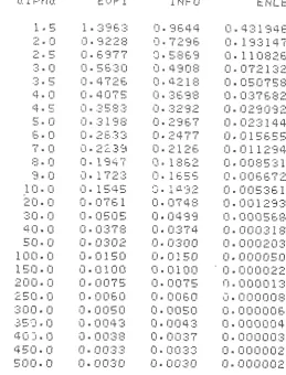
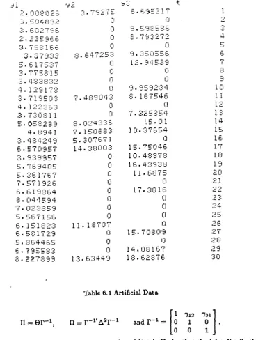
In Chapter 6 two tractable multivariate models are formulated. Section 6.1 introduces a general

recursive model analogous to the fully recursive econometric models (Zellner, 1971). In Section 6.2 an

example using artificial data illustrates an application to nested missing observations. In Section 6.3

we make use of the discount concept (Ameen and Harrison, 1983; Harrison and West, 1986) in order

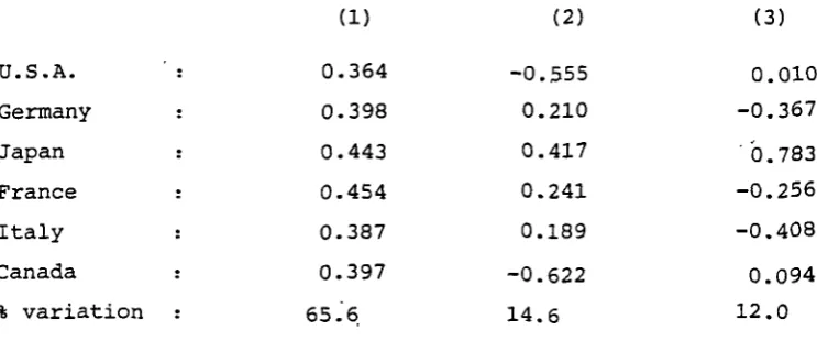
to simulate a DLMR with a dynamic scale variance. In Section 6.4 we compare the performance of

a DWMR, with a dynamic scale variance matrix, to its static counterpart using exchange rate data.

In addition, we employed PIE's for estimating the principal components of the scale variance matrix.

This provides an insight into exchange rate dynamics. The use of simulation in Bayesian statistics

is discussed in Appendix A6.1. This material is employed in the example of Section 6.2. A result

concerning the distribution of swept matrices is provided in Appendix A6.2.

Chapter 7 is devoted to modelling aspects. The setting of vague priors for the DLMR model is briefly discussed in Section 7.1. The use of the multivariate logarithmic and logarithmic ratio transformations

in the context of DWMR modelling is the topic of Section 7.2. Section 7.3 concerns alternative but equivalent reformulations of the DLMR model which expand its field of applications. The models

and error, fixed-lag smoothing and prediction, differencing series and transfer response functions.

Finally, Chapter 8 consists of a general discussion and possible topics for further research.

The thesis is written in an informal style; the results presented are justified rather than rigorously

proved.

1.5 NOTATION.

Throughout the thesis the following notation is employed unless otherwise specified. Scalars are

denoted by lowercase letters (v, w, . . .), column vectors by underlined lowercase letters (x, y, ... ) and

matrices by uppercase letters (X, Y, ... ) and unknown parameters by Greek letters (8, E, ... ). The

factorial symbol ! is used in a extended sense, i.e. x! denotes the gamma function evaluated at x + 1,

and the symbol

r

is reserved to denote the gamma distribution. The digamma function - the derivative

of the (natural) logarithm of the gamma function - is denoted by 6(x).

Expressions like a- 1A are often denoted by del, . Conformable matrices are partitioned preserving the

conformability within the submatrices, e.g. in the expression

[A Bl[E F 1,

the products AE, BC, AF, BH, CE, DC, CF and DH are implicitly assumed to be well defined.

Simi-larly, in the expression

[ Ac B1 + {EFG ],

the sums A + E, B + F,C + G and D + H are assumed to be well defined, etc. In addition, we use the [A 0 0

diag operator for denoting block diagonal matrices, e.g. diag(A, B, C) = 0 B 0 .

0 0 C

In order to simplify the notation common conditional information is often omitted as in the

specifi-cation of the dynamic model in Sections 1.2-3, e.g. the model (1.2) is implicitly assumed to be

p(Ot iHt_ i) = f p(Ot let _ i ,Ht _ 1) p(Ot _ i lHt_ 1) d9_1,

et-i

gYti llt- 0 = f gYtlet,llt-1) p(O t Ilit_4) det , and

et

p(Ot lyt ,Ht _ i) = P(Yti9t,Ht_i)p(9t1Ht_i) P(Yt IHt-i)

where Ht _ 1 stands for the relevant information known up to time t — 1. The random variables on

which operators such as mean and variance depend are included in the notation as subscripts, e.g.

Eo f (x) = f f (x)p(x10) dx.

z

Our notation and terminology for the models described in the following chapters is a compromise

between the conventional notation and terminology in Bayesian forecasting and econometric literature.

As any compromise, this has advantages and disadvantages depending on one's point of view. Further

notation is introduced when needed, in particular in Appendices A3.1, A3.2 and A4.1.

CHAPTER 2

THE DYNAMIC LINEAR MODEL

Since the introduction of the Dynamic Linear Model (DLM) by Harrison and Stevens (1976), Bayesian

forecasters have made use of an appealing dynamic model which can deal with multivariate time series.

The DLM offers many facilities: use of prior information to start up the system, construction of

com-plex models from simple components with the aid of the superposition principle, intervention analysis,

discrimination between rival models, simple sequential updating recursions, joint forecast distributions,

time invariant interpretation of the system parameters, and so on.

In this chapter the DLM is reviewed and a basis is provided for the next chapter where an extension of

the DLM, the Dynamic Linear Matrix Regression Model (DLMR), is developed. The DLM description is given in Section 2.1, the updating recursions are provided in Sction 2.2, time invariant interpretation

of the parameters and model building from simple components are the topics in Section 2.3, Multivariate

DLM's are entertained in Section 2.4, and the problem of specification of the evolution variance and

observational variance with emphasis on the multivariate case is discussed in Section 2.5.

2.1 MODEL FORMULATION.

The assumptions of the DLM of Harrison and Stevens (1976) for a multivariate time series Et are:

Observation Equation:

Evolution Equation:

Prior Information:

Where,

x

t

e

t

+

ft , gt N (Q, Vt).

= Gt2t _ i + ft , ft N(0, Wt).

N(_ 1 , C_1).

is the tirne index (t = 1,2,3, ... ),

yt is a (r x 1) vector of observations made at time t, Xt _{is a (r x p) matrix of independent variables,} 0

—t is a (p x 1) unknown vector of system (regression) parameters, At is a (r x 1) observation error vector,

Vt is a (r x r) variance matrix associated with et, Gt is a (p x p) evolution (trend) matrix,

f is a (p x 1) evolution noise vector,

Wt is a (p x p) variance matrix associated with

As usual, N(m, C) denotes the multivariate normal distribution with mean

m

and variance C.

The equation (2.1a) defines the distribution of the observations y t given the system parameters. The

system dynamics are determined by (2.1b) which specifies the distribution of the regression coefficients

- N(mtk , C7), where c7 = W + _{and tii = Gtmt—i.}

N(91t, kt ), where kt = Vt + XtC7X1 and =Xm.

641 4 N(,Ct), where ct = - At f'tA,m =

t = and At = GTXA-1. Prediction:

Posterior:

(2.2a)

(2.2b)

(2.2c) the distribution of the regression coefficients at time t — 1. The distributions appearing in (2.1) are

implicitly assumed conditional on the relevant information available at time t — 1 including (if any)

previous observations mt_2, .... It is further assumed that_e , t ft and are independent, with

ft , ft independent over time.

The following terminology is employed. When Xt, Gt, Vt and Wt are not dependent on time then the DLM is called a constant DLM. If in addition W = 0, then a DLM is referred to as a noise-free constant DLM.

2.2 UPDATE COMPUTATIONS.

When a new observation is obtained we have to revise our beliefs about the parameters (and implicitly

our beliefs about the forthcoming observations). It is sufficient to describe this updating process for

just one observation, since it can be performed over and over again when more observations become

available, in a sequential fashion which is characteristic of the Bayesian approach. The updating recursions for the DLM are:

Evolution:

Equation (2.2a) provides the distribution of the regression coefficients at time t conditional to the

information available at time t — 1. The one-step ahead predictive distribution of 4 made at time t — 1 is given by (2.2b). The regression coefficients distribution at time t updated with the additional

information is provided by (2.2c) completing the system cycle.

The derivation of (2.2) is a simple exercise of multivariate normal theory, this is not done here, but in the next chapter the updating recursions for the DLMR, which contains the DLM, are obtained.

The system (2.1) is in probabilistic terms equivalent to the Bayesian formulation of the Kalman (1963)

state-space model found, for example, in Aoki (1967) and Maybeck (1979). The counterpart of (2.2) is

known as the Kalman filter in engineering literature.

The recursions (2.2) provide a very convenient way of updating the system. The statistic (together

with Ct ) is sufficient for t at time t and summarizes all past information. Thus, for forecasting purposes, it is equivalent to the whole previous history of the system. The implementation of (2.2)

may be done in a straightforward manner with the possible exception of (2.2c), which requires, in the

multivariate case, the computation of the matrix inverse of kt . The square-root algorithms found in the

where

Gt and Wt = [W11 W12

1

W21 W22 t

—

1\ f.

= — 1) 3.)1

= 1

3• • • ;PI

(2.3)

Kalman filter literature, see for example Maybeck (1979) and Anderson and Moore (1979), are useful

for dealing with systems requiring high precision. Perhaps the easiest implementation of (2.2) is by

means of the Efroymson (1960) sweep operator. These implementation aspects are covered in Chapter

4.

2.3 STANDARD MODELS.

In state-space modelling the aim is to make inferences about the past, present and future (smoothing,

filtering and prediction) of the system state f t , which usually has a physical meaning. In contrast,

Bayesian forecasting is concerned, primarily, with the distribution of the future observations based

on the available information. The vector parameter ft represents time varying regression coefficients

which, in the standard models, have a time invariant interpretation and play a very important role in

understanding and operating the system.

2.3.1 Superposition Principle.

The superposition principle is a simple, but powerful statement, which tells us that a linear

combi-nation of DLM's is itself a DLM. In particular, it means that the trend of the series E t given by Xtft

and ft = GtOt—i +IA can be constructed as the sum of simple trends, i.e. two trends

X

i

t Oit , 4t

=

+ lit, N(0, W), i = 1,2 can be combined into

Xtlt

=

Gt/t _ i +Litt, tit .-•-• N(0) Wt)

1 °it

XtOt = [X1t1X2t1 = X2tti2t, -2t

{G11

0

G22 1t

0

The generalization for several trends is evident.

This facility is very useful since it provides a method for building up complex models from simple

components, and it is employed in one form or another in many models appearing in the following

chapters.

2.3.2 The Polynomial Trend.

A univariate DLM with polynomial trend of degree p — 1 can be constructed by taking X t = X

=--[1,0,... , 0] and Gt = G

a

right triangular matrix such that the non-zero triangle is precisely the Pascal

triangle (from left to right), i.e.

where (i _ _{j) means 1 if i j and 0 otherwise. A key property of G, shown in Appendix A2, is the}

following:

• - . < j_i i

= _—

₁₎

— .7)8 _{= -;•••,P•}1

wit

Notice that the elements of the first row of G8 are the powers of s, i.e. 1, s, . . . ,

For convenience we consider first the noise-free DLM i.e.

gt = Glt—r• (2.5)

In this case, from (2.4) and (2.5) it is clear that the trend is given by

XIt+ . = • - • = [1, (s — 1), ..., (s — 1)17-1104+1 = [1, s, . .. , 3P-1]Bt (2.6)

Therefore, the trend has a polynomial form and the parameterli t represents the polynomial coefficients

relative to the system of coordinates with origin at (0, t).

If the noise-free assumption is dropped, then the parameters have random disturbances but the

previous interpretation remains valid by substituting the parameters with their expectations, i.e. the

forecast function (the mean of yt+, conditional on the information available at time t) is given by,

Ft (s) = X _i_ i, -= • • • = [1, 8, ... , 3P-11mt. (2.7)

It should be noticed that other representations are possible, for instance, taking

X = 11,0,—, 01 and G = I ±

2 0 OI'

gives the Jordan-canonical form based on the standarized factorial polynomials (I), CD, ... , (° 1) rather

than on the powers of s.

2.3.3 The Harmonic Trend.

Proceeding as before, a univariate DLM with simple harmonic trend of period 27r/w can be constructed

by taking

Xt = 1= [1,0J

The counterpart of (2.4) is

cos w sin w and Gt = G =

— sin w cos w •

cos w s sin ws

G8 = (2.8)

— sin ws cos ws '

which may be derived easily using the well-known trigonometric formulas for the addition of angles.

Again, we first consider the trend of the noise-free DLM. It follows from (2.5) and (2.8) that the

trend is,

Xit+, = • • • = [cos (.4)(8 — 1),ins w(s — 1)] 2 = cos ws , sin ws] [[ 0, 1 ] .

r0i Li v2 t

(2.9)

Thus, the trend consists in a single harmonic and Olt, 02t are the coefficients associated with the cosine

and sine components relative to the system of coordinates with origin at (0, t).

As before, this interpretation remains valid when the noise-free assumption is dropped, if the

param-eters are substituted by their expectations, and the forecast function is,

Ft (s) = [1,0] [ • rni i = • - = [cos ws, sin ws][nli . (2.10)

rn2 t_+s M2 ] t

Complex harmonic trends with several harmonics are achieved easily by means of the superposition

0

+

0 X22 t t ez

t'

t

N (

(2,

V12 V21 V22 t

V 11

t

(2.12a)

r1

[Gil

₀

₁

_ill

₁

_W12

I

.

:

2

i

t

N

(11 [

w W 3.1

21 W22 t)

±

Le2

i t

L 0 _{G22 J t L (12 J t-1 LI2Jt}

tjut

(2.12b)

and a trend matrix diag ([

₀

1 diaga1,01, [1,00)

2.3.4 Damped Trends.

A damped version of a trend given by X

t

= X and Gt = G is constructed by taking AG as the new trend matrix instead of G, where A is a suitable scalar typically 0 < A < 1.

The mixtures of polynomial, harmonic and damped trends constructed with the aid of the super-position principle provide a very rich stock of models, certainly wide enough for the purposes of this thesis.

2.4 MULTIVARIATE MODELS.

All standard models discussed so far are univariate models. However, one version of the superposition principle provides a method for building-up multivariate DLM's from univariate DLM's.

Two multivariate DLM models for y y2t,

Y..

t

= —N(, V

1 ),

i= 1, 2, (2.11a)

= + N(, W11 ), i

= 1,2,

(2.11b)

can be combined into a single

DLM for MI ,

t

The generalization for several components is easily appreciated. For instance, a trivariate DLM, with a linear, simple harmonic and damped constant trend for the first, second and third dependent variables respectively, has a regressor matrix

1 cos w sin co 1 ' — sin cos co A) •

A simple but very useful DLM for time series in which all the variables have a similar trend deter-mined by X

t

and G

t

, has a regressor matrix diag(X,... , X) and a trend matrix diag(G,..., G). The importance of this class of models becomes apparent in the following chapters.

2.5 SPECIFICATION OF THE VARIANCES.

In order to implement a DLM, practitioners face a major obstacle: the setting of two system variances

Wt and V. The first difficulty has been overcome partially by Ameen and Harrison (1984) through the

discount concept which substitutes the evolution variance matrix Wt by a set of discount factors and

offers a conceptually simple alternative model. Nevertheless, the specification of the observational variance V

t

for multivariate DLM's remains a major problem for practitioners.

2.5.1 The Discount Weighted Version.

The DLM version, based on the discount concept, merely substitutes the first equation in (2.2a) by,

= (diag /1)

-

Gt Ct _ I G't (diag - (2.13)

where 13 is a set of discount factors, i.e. each element of 13 lies between 0 and 1.

The advantage of using the discount version over the standard version is clear; the specification

of a rather cumbersome variance W

t

is traded for a set of discount factors for which many practi-tioners have a natural feeling. Often a discount model can be interpreted as

a

DLM; however, the equivalence between a discount DLM and a standard DLM is not always guaranteed, i.e. the matrix

_1

(diag§.) - 4 GtCt_ i Gl(diag L.3) 2 - Gt Ct _ iq fails sometimes to be a proper variance. Furthermore, the

equivalence, for an arbitrary discount set t3, is guaranteed if and only if GtC

t

_

i

C

t

is diagonaL The discount version may be modified, in order to assure equivalence by adopting the following rule

instead of (2.13),

2.5.2 On

-

line

Variance Learning.

A

natural alternative for avoiding the specification of the observational variance is to assume that it

is unknown. This approach, in the univariate case, replaces the model (2.1) by

1371 •

if .

=

14 2

{ A-i t ' fi1 3 ' (.)

otherwise

where B

t

= Gt Ct_ i G't .

A

parsimonious form for independent components recommended by West and Harrison (1986) is to take the same discount factor within elements of each component. This procedure

is referred to as discount

,

by blocks. In some circumstances it is useful to combine a discount procedure

followed by the addition of a noise variance.

Observation Equation:

Evolution Equation:

Prior Information:

Yt = 42: + et, et N(0, o-

2

vt ) (2.15a)

e

t = ft- N(0,

cr2

Wt) (2.15b)

""' N (—mt-11 Cr2Ct-1) and cr2 •-•

r- I ( I dt_i, tst-o•

(2.15c)

Where cr

2

r-- 1

(d, is) means that CI

-2

has a gamma distribution with mean -1-: and varianceId

2

It is implicitly assumed that the distributions in (2.15a), (2.15b) and in the left-hand side of (2.15c) are

conditional on o

2

and also, of course, on the relevant information available at time t — 1. Henceforth

0

we denote the joint distribution induced by (2.15c) as [-t

cr2

-

1 ,--,

N

r-i(_. 1 ,

C..1,Idt-i, ist-i)

and

the marginal distribution of as '''

t

(

m

t-i, st-i

e

t-i dt-i)•

Using the recursions (2.2a) and (2.2c) for O t la2 and (2.2b), together with a direct application of

Bayes' formula for o2 , the following updating recursions are readily obtained,

Evolution:

Prediction:

Posterior:

where mi'`, C7, 9,,p,, et are

VT

it ]Nr-1(m:,q, ;4_1, 4 st_1)

Yt '" t(ts st—igt, dt—i)

r2] lYt '''' N

l'-'(mt,ci,

I dt, I st)

as in (2.2) and cit = cit _ 1 + 1,st = 3t _ 1 + e2/t.

(2.16a)

(2.16b)

(2.16a)

Clearly, for o2 = 1 the model (2.15) becomes a conventional univariate DLM. Therefore, it is an extension of the DLM model and describes essentially the model employed by Smith and West (1983),

a non-Bayesian formulation can be found in Harvey (1984). It is important to notice that, for v t = 1, o2 is not only the unknown observational variance but it also appears as a scalar factor in the evolution variance.

The above procedure can be easily extended to the multivariate case when the observational variance

is assumed known except by an unknown scale factor, and it is found in West (1982). Unfortunately,

any attempt to leave the observational variance unknown as a whole in the multivariate case faces the

problem of intractability, the reason being that the generality of the likelihood rather than the dynamic

structure of the model. For instance, the static DLM leads to an intractable analysis as is shown in the next chapter. Hence, the specification of the observational variance in the multivariate case remains a

major obstacle. Furthermore, one of the main objectives of an analysis may well be to learn about the

APPENDIX A2.1.

THE POLYNOMIAL TRANSITION MATRIX.

The representation of a polynomial trend in terms of powers of s, although natural, is not common in Bayesian forecasting. For this reason we give a derivation of (2.4).

The formula (2.4) may be verified by means of double induction, on p and s, as follows. Let

Gs GIV GIV

0 J

then it is enough to show that

fc

_ii G 112).

1 G

J. —1) G i8-2 1 ) G (181) G(8) 1

10 i i i. J o

J'

but G18/) G181-1) = G(3.1). by the induction hypothesis on p, and using the binomial theorem it is clear that

G111) G(1.2-1) ± Gii2)=[(3.

—1 1) (1<— (P (a — 1 ) P- 1 ± [(I)— 1)]

i _{— 1 i 1}

{ p-1

-

Ee.iiii)(Pil(s-ir-l+r11)

2 =2

p-1 ix ix

1 ) (1; 2) (3 — i)P-1 + (Pi 1 11)]

P—i

= [0 — 1.)

v, —

1) fa G

(8)

— 1 ) Z' j=0 )‘ 12

(1.1(P-1) s-1 j-1 = (1's— 1 p-3, •

CHAPTER 3

DYNAMIC LINEAR MATRIX-VARIATE REGRESSION

This chapter is concerned with a dynamic linear model proposed in Quintana (1985), which extends

the DLM by considering matrices of observations, instead of vectors, and introducing a new system

scale variance matrix. In doing so, the dynamic structure of the DLM is transferred to the new model

which includes the standard multivariate regression model, with the observational variance unknown,

as a special, static case. This matrix-variate model is referred to as the Dynamic Linear Matrix-variate

Regression (DLMR).

In 3.1 the intractability of the static DLM with an unknown observational variance is shown, the

DLMR is suggested and the description of the DLMR is given. Its updating recurrences are derived in

3.2. Static and dynamic models contained in the DLMR, a vector representation, a discount version and

model building facilities inherited from the DLM are entertained in 3.3. Finally, multi-process models,

reparameterization and system decoupling are discussed in Sections 4, 5 and 6 respectively.

Henceforth several results of the vec operator, Kronecker product 0, and matrix-variate distribution

theory are invoked freely. Definitions and properties of the Kronecker product and the vec operator are

provided in Appendix A3.1. The essential singular and non-singular matrix variate distribution theory

is developed in Appendix A3.2.

3.1 MODEL FORMULATION.

In this section we confront the difficulties associated with the DLM when the error variance is assumed

unknown. Then, perceiving how the problem is overcome in the static case we formulate a tractable

dynamic model.

3.1.1 Static and Dynamic Models.

In Subsection 2.5.2 it is claimed that the static DLM with the constant variance V unknown leads

to an intractable analysis. This may be shown as follows. This static model is the DLM (2.1) with

Gt = I, Vt = V and Wt = 0 for all t, i.e. its observation equation is given by,

& = Xt 0 + Et , t = 1, ... , n, ft — N(0, V). (3.1a) It can be rewritten in the matrix form

Y = X8 + E, E ,--, N(0,V, A _(3.1b)

i

ef

iS

where Y = [y1 , ... , y ] a (r x n) matrix, X = [X1 , . . . , Xn] is _{a (r x (pn)) matrix,}

e = -r

a ((prt) _{x n) matrix, I is a (n x n) matrix, and E = [el, • • • ) e I is}

a (i

i

i x

r4) _{matrix. Therefore the}

likelihood is such that (see A3.2.10)

p(Y12, V) oc 11, 1 - 11 exp(— I tr(EVY-1)).

N

(

[ -r

T]

[ C(; 1 PC)Vti)

since

and

Problems arise because there is not in the general case a tractable sufficient statistic; see Section 1.3.

This difficulty is essentially the same as that found in related static linear models such as the general

linear model with common regression coefficients (Box and Tiao, 1973, p. 501-502) and the seemingly

unrelated regression (Zenner, 1971, p. 240-243). Furthermore, let us assume that the variances in the

dynamic model (2.1) are constant (Vt = V and Wt = W for all t) but unknown with independent

inverted-Wishart distributions. In this case it can be shown that the posterior distribution of It is an

intractable multivariate poly-t (Broemeling, 1985, p. 286-290).

Hence, it is clear that extra assumptions are necessary in order to obtain a tractable procedure

for on-line variance learning. The artifice for the static case is well-known; the standard multivariate

regression is considered as an alternative to a more general model such as the generalized weighted

multivariate regression model. Both models can be embedded in the matrix model,

Y = X8 + E, E (3.3a)

with the conjugate joint matrix-normal inverted-Wishart prior for

e,

E given by

8 •••-• N(M, C, E) and (3.3b)

E W-1 (S,d). (3.3c)

It is further assumed that 9 and E are independent given E.

Taking V = I we have the standard multivariate regression with the observational variance E

un-known. When Y is a column, and X = diag(Xi, Xi ), we obtain the weighted generalized

multi-variate regression where the observational variance VY.: is known except for an unknown scalar factor

E; compare with Press (1982, p. 245-248).

To see how the discussion of the static case brings some insight to the dynamic case, we have to

realize that a dynamic model can be thought of as a static one by considering the evolution and the

prior as a joint prior, e.g. the DLM (2.15) can be seen at time t as,

y =X1-1-e, a2V), (3.4a)

— N(11, 02 C), (3.4h)

where

r

[Gt

'fl.

-Q

= /t e

d C =

ol

an

lot

'IL

0

V=V,

oil'

wt LGt I

The representation (3.4) of the DLM (2.15) suggests that we consider the model (3.3) at time t where

Yt, X = [0, Xt l,

e [

e

4-

t

i],

E = Et , V = Vt)

M

=

1

A-1

1

GtMt—

Ct-1 Ct—iCit 1

C=

Gi Ct- 1 Wt S = St—i and d = dt—i,

i.e.

Observation Equation:

Evolution Equation:

Prior Information:

(3.5a)

(3.5b)

(3.5c)

y

t

xtet +Et,

Et N(0, Vt,

et . ctet_i +Ft,

Ft N(0, Wt, E).

[et_ii Nw-

_I

_(Mt-i,

_{Ct—i, g- t-1 1 dt-1)•}

Where Et , Ft and

et_

1 are independent (with Et , Ft independent over time) given E; see A3.2.8.

3.1.2 Model Description.

Throughout the thesis the model (3.5) is referred to as the Dynamic Linear Matrix-variate Regression (DLMR) and the following notation is used:

Yt is a (r x 9) matrix of observations made at time t,

It _{is a (r x p) matrix of independent variables,}

et is _{an unknown (p x q) matrix of system (regression) parameters}

Et is _{a (r x observation error matrix,}

Vt is a (r x r) variance matrix associated with Et 3 Gt is a (p x p) evolution (trend) matrix,

Ft is a (13 x q) evolution noise matrix,

Wt is a (p x p) variance matrix associated with Ft , and • Is a (9 x g) system scale matrix.

The matrices Xt,Vt, Gt

that E is unknown with prior inverted Wishart distribution, at time t —1 (after Yt _ j. is observed), given by

E di....') (3.6a)

in accordance with (3.5c). However, in some circumstances it is convenient to assume that E is given.

Naturally in this latter case,

et_ i N(Mt- Ct--1, E), (3.6b)

since (3.5c) and (3.6) are equivalent by definition; see A3.2.17.

Several useful static and dynamic multivariate models are embedded in this model, a list is given in Subsection 3.3.1. The role of E as a matrix scale factor is analogous as that of o2 in model (2.15). This is discussed in Subsection 3.3.2.

and et= IGt

i

ret-11

_F

_{t J}

3.2 UPDATE COMPUTATIONS.

Our goal is to derive and to analyse the asymptotic behaviour of the the DLMR updating recursions analogous to the recurrences for the DLM. These resulting recursions enable us to perform the process

of incorporating the information of the observations in the usual sequential fashion.

The most economical way of obtaining the sequential updating recursions for the DLMR is by

borrow-ing the DLM results as istQuintana (1985). However, here we prefer to give a self-contained derivation based on the results shown in Appendix A3.2.

3.2.1 Updating Recurrences.

First let us derive, for convenience, the recursions analogous to the formulas (2.2). Assuming that E

is given, the updating recursions for the model (3.5a), (3.5b) and (3.613) are as follows.

Evolution:

et

N(Mt* , E), where CT = Wt + G

t

C

t

_

i

Gi

t

and Mt* = Gt Mt _ i . (3.7a)

Prediction:

Posterior:

Yt N(kt , E), where kt = V

t

+ X

t

C;Xl and

kt =

Xt Aft* • (3.713)

where Ct = — Attle

t

, Mt = Aft" + At t

etlirt-N(mt,ct,E),

(3.7c)

= Yi -

Pi and At = Ct*.70t-1.

These recursions may be shown as follows. Using the independence of et _ 1 and Ft together with (3.6b),(3.5b) and (A3.2.5) it is clear that e t is distributed according to (3.7a) since

[et_11

N

(rAft_il 1ct_1

01

_E)

F

t

\I. 0 .1 1 L 0 Wt

Following a similar argument, (3.7a) and (3.5a) imply that

[7;t1-

F'

rEttl

and

[et ] Et

-N(rg ,

[ Cciv0t1,E), i.e.

[ E:rit N XM

t

il*

fd

'[X

c

t b; Xt

CC; tJC* ft-Fr Vt] ' (3.8)

Thus, the prediction and posterior equations (3.713) and (3.7c) are simply the relevant marginal and

conditional distributions of (3.8) according to (A3.2.8).

The recurrences (3.7) provide a recursive algorithm for updating the system since Mt and Ct

sum-marize all present and past information at time t. It is of note that neither Mt nor Ct depend on E. So far, the recursions (3.10) are valid for any proper variances Vt , Wt, Ct—i and E, i.e. they may be

singular, Only kt has been implicitly assumed non-singular, but even this requirement is abandoned in Section 4.2.

We now drop the assumption that E is known and instead it follows an inverted Wishart distribution

at time t — 1 given by (3.7a). The conditional distribution of EIY2 is implicitly given by (3.7b) and

(3.6a), since according to (A3.2.17),

[E ] ,--, NW

t

-1

(2,2, St-1, and applying (A3.2.19) we have,

Elli — W-1(St,dt),

(3.9)

where,

St = St_ i + EC4

-1

E2 and c/2 = 4_ 1 + r

Therefore, the recurrences (3.7) may be generalized for the model (3.5) as follows.

Evolution:

Prediction:

Posterior:

[ e

E --,

t

J

NW

-1

(M:, C:, St— ii dt— 1)•

Y2 ,--. T(t, tiSt-1,4-1)•

r Et

I l

l'

t

-

Nw -1(mt, ct, st,dt).

Where M:, q, Pi , Pi , Aft , ct , Et and A2 are as in (3.7), and St , dt are as in (3.9).

Similar comments as those following the derivation of recursions (3.7) apply to (3.10), in particular, (3.10) is valid even if S (E) is singular. The essential difference is

that (3.9)

provides an effective procedure for on-line learning about the system scale variance E. Long-term forecasting can be achieved

by means of repetitive use of (3.10a), (3.10b) and replacing the recurrence in (3.10c) by C 2 = C:

and M2 = M: (provided, of course, that the driving parameters Gt+,,Wt+, and the observational parameters Vt+, and Xt+„ are known for a = 1,2, ... ).

3.2.2 Limiting Behaviour.

For simplicity we look first at the case for E known. The resemblance between (3.7) and (2.2) is

evident, in fact (3.7) becomes (2.2) when E = 1. Moreover, the behaviour analysis of C 2 and A2 can be

reduced to that of the DLM because from (2.2) and (3.7) clearly Mt , C2 , )12 , etc., are computed exactly

as if the columns of 1/2 were driven by DLM's with common parameters IC2 , Gt ,Vt and W2 , regardless of the actual E.

A particular but very important case is the observable constant DLMR. This case is obtained when the associated DLM's, described in the previous paragraph, are observable constant DLM's, i.e. when

X, G, V, and W are not time dependent and there is a vector A such that,

[ hl'X'ICIC

-•

is a full rank matrix. In this case A t , Ct , Cik and kt converge because the result holds for the DLM, for a simple proof of the latter see Harrison (1985). If the DLMR is unobservable, then only partial convergence can be assured, see again the reference above for details.

These results still hold when E is distributed according to (3.6a) instead of being known, since the behaviour of Mt , Ct , At , etc., is independent of the actual E as is mentioned in Subsection 3.2.1. However, in this case it is interesting to look at the behaviour of S t and de as t increases. From (3.9) we obtain,

St

so +

and dt = do ±

tr

(3.11)

r=1 St

Therefore, in the limit, E = lim 2 in probability and (3.10) becomes (3.7).

t-.03 dt —

These limiting results may be employed in oder to reduce the update computations for a constant

model after a period of time. Typically, the convergence is fast and the recursions (3.10) may be

replaced by to Mik = GM- 1 , Y = X Mt* and Mt = Mt* ± A(Yt — kt), where A is the limiting value of

At.

3.3 THE DLMR

AS A

DLM.

Modelling with the DLMR essentially can be reduced to modelling with the DLM because most of

the DLM structure is inherited by the DLMR. In this section it is illustrated how this transference can be done. First, we look at some standard multivariate linear models which are embedded in the DLMR.

3.3.1 Models Contained.

The DLMR contains a wide variety of normal linear models which can be divided into two main

categories: dynamic and static. By a static model we mean a DLMR which is not evolving at all i.e. Gt = I and Wt = 0 for all t. The particular settings are as follows.

Static Models:

(a) Standard Multivariate Regression. This model can be seen either sequentially as a DLMR with r =

l

and Vt = 1 for t = 1, ,n, or in its entirety as a DLMR with r = n and Vt = I at a fixed time

t = to.

(b) Weighted Generalized Multivariate Regression. This model as defined in Press (1982) corresponds

to a DLMR with q = 1 at a fixed

time t = to. A

classical interpretation of the hyperparameters Mt, Ct and St is given in the next chapter.

Dynamic Models:

(a) Dynamic Weighted Multivariate Regression (DWMR). The DWMR generalizes the Standard

Multivariate Regression and corresponds to a DLMR with r = 1. Therefore, it is a very important case

of the DLMR and it is discussed in Section 3.7.

(b) Multivariate Dynamic Linear Model. The DLM's correspond to DLMR's with q = 1 and therefore E = 0.2 is a scalar. For the Harrison and Stevens (1976) DLM, o.2 is assumed to be known and

equal to one. For the multivariate extension of the DLM (2.15), cr 2 is assumed unknown and cr 2 -,

r -1 (d_1, i8t—i).

Thus, the DLMR can be thought of as a combination of extended DLM's and DWMR's. The columns

of Yt are being modelled marginally as extended DLM's with common parameters X t , Gt,Vt and Wt

whilst the rows are marginally modelled as DWMR's, where their parameters are the corresponding

rows of Xt and diagonal elements Vt , and common evolution parameters Gt and W. These comments

give full support to the discussion in the previous section. In accordance with the terminology of the

static and dynamic models the DLMR is referred to as weighted or non-weighted depending on Vt (this must not be confused with the discount weighted method of Subsections 2.5.1 and 3.3.3).

The DLMR not only provides a theoretical framework for the models mentioned above, but also

makes possible the implementation of a relatively simple program suitable for a common personal

microcomputer which can handle all these models at once as is shown in the next chapter.

3.3.2 Vector Representation.

Readers already familiar with the DLM may find a vector representation of the DLMR more easily

interpretable. Applying the vec operator on (3.5a), (3.5b) and (3.6b), and using properties listed in

Appendices (A3.1) and (A3.2) we can readily rewrite the model (3.5) as,

Observation Equation:

vec Yt = (I 0 Xt ) vec et -I- vec Et, vec Et ,-.., N(0, E 0 Vt).

Evolution Equation:

vec et -= (I® Gt) vec et_ i + vec Ft , vec Ft ,-, N(0, E ® We). Prior Information:

(3.12a)

(3.121))

vec et_ li E ,-.. 14(vec Mt_ i , E 0 Ct_ i) and E -, W-1 (St-I, dt-1) . (3.12c)

The representation (3.12) implies that, given E, the DLMR is a special case of the DLM (2.1), in

which the driving parameters have a special structure given by the Kronecker direct product: E is a

scale factor of the variances and I is a scale factor in the linear transformations. This shows the richness of the DLM and DLMR since, given E, each is a special case of the other!

The vector form of the DLMR is very useful in order to transfer the structure from the DLM to

the DLMR. For instance, it is apparent from (3.12) that dropping the assumptions about normality,

et = Mt and ke = Xt et are the best linear estimators in the linear Bayesian sense (Hartigan, 1969), regardless of whether E is known or not. As mentioned before the DLMR updating recurrences (3.7),

given E, may be derived using the DLM recurrences corresponding to (3.12) and switching back to the

3.3.3 Discount Weighted Version.

The interpretation of the DLMR as a combination of extended DLM's and DWMR's given in Sub-section 3.3.1 suggests the use of the same discount factors )9 for each column of e t . Thus, according to (2.13),(3.12) and (2.2a), the discount version substitutes,

(E Wt) + (I® Gt )(E 0 C)(1. Gtr = E 0 (Wt GeCt _ i G) = E

by,

(E Ct )* = (I 0 diag (I Gt )(E 0 Ct _ i)(I Gt )' (I diag fir I

= E (diag fir Gt Ct _ i G1 (diag fir = E C7,

i.e. the first equation in (3.7a) is replaced by (2.13). For the reasons expressed in Section 2.5.1, the use

of the rule of discount by blocks (2.14) is recommended instead of (2.13).

The analysis of the limiting behaviour can be reduced, in a similar manner as with the usual DLMR, to that of the DLM with a discount version found in Harrison (1985). For instance, an observable

constant discount DLMR converges, etc.

3.3.4 Model Building.

Two aspects need to be considered when constructing a DLMR model: trend and variance structure.

The standard trend models of Sections 2.3 and 2.4 can be built in a straight forward manner. It is only

necessary to keep in 'mind that Xt and Gt determine the common trend form for the columns of Y.

For instance, the setting given in Section 2.4,

Xt = diag([1,0], [1,0],1) and Gt = diag 01 r cos w since A) ([0 1 ' sin w COS CV

for a DLMR with r = 3,p = 8 and q = 2 means that the three bivariate rows of Yt have a linear, a simple harmonic and a damped constant trend respectively.

Regarding the variance structure, Vt , Wt and Ct retain essentially the same meaning as with the DLM; Vt represents the inverse weight or precision of the present information, Ct_ 1 measures the

inverse weight of past information, and Wt controls the inverse weight of the link between past and

present information.

In practice it is helpful to remember that Vt , W, C_ 1 and the columns of Yt steer Ct and mt with the DLM recurrences (2.2). In particular modelling with a DWMR is essentially as easy (or difficult)

as modelling with univariate DLM's.

Special models such as those with correlated error and noise, time correlated noise, transfer response functions, etc., are discussed in Chapter 7.

3.4 MULTI-PROCESS MODELS.

It is often the case that a modeller has in mind two or more possible models for a certain time series; to handle this, Harrison and Stevens (1971, 1976) introduced the multi-process models methodology for

discriminating between rival DLM's. Two situations are considered; multi-process models class I deals

with fixed DLM's whilst in multi-process models class lithe possible DLM's may change from one time

interval to another following a Markovian scheme. The technical details of multiprocess models for the

DLMR are given in this section.

3.4.1

Class

I.

Suppose that we are considering a set of possible DLMR models .h.1 (1) (i = 1, 2, ... , m) for describing

the time series Yt (t = 1, 2, ...). In addition, we believe that at least one of these models is adequate, but we do not know precisely which one is. Our problem is to discriminate between these rival models. Let Pt (M (i)) denote the probability that the time series follows the model /A P given all information

available at time t but prior to observing Yt , and Pt (.M (i) lYt) the revised probability given the additional

information Y. Then, the two probabilities are related according to Bayes' theorem as follows,

Pt( MM I Yt) cc P( YtI M(i) ) Pt 1)4(i)), (3.13)

where p(YtlX(i)) denotes the predictive density for Yt assuming the model M ( i), given all information

available at time t.

The applicability of (3.13) depends on the existence of the predictive density for

Y.

But for the DLMR this is obtainable either from (3.7b) or (3.10b) depending on whether E is known or not. Therefore, the recurrence (3.13) 'provides a means for an effective on-line model discriminating procedure.

The possible DLMR models can be completely arbitrary; typically each .M( 1) has its own associated

parameters 4i) , , wt(i) for t = 1, 2, .... The multi-process models class I offer a simple method

for tuning constant DLMR's provided, of course, that the number of the rival models (m) remains

manageable.

3.4.1

Class

II.

Now we turn to the case in which a fixed DLMR may not adequately describe the time series. Instead

it is assumed that the model may switch from one time interval to the next in a Markovian fashion.

Let ,MV) (5 = 1,2, ..., rn) denote the assumption that the evolution and observation of the process at time t is defined by 41) , Vt(i) , GV) 431. The Markovian transition of the process is described by

P ( M ii) I Mli)1), the probability that the process swings to 14 1) from .M 1 . A classic example of a system with a linear trend is to consider four models: the first is a default model which describes the system most of the time and three alternative models which represent an outlier observation, a step

change and a slope change, by means of a suitable setting of Vt(i) and Wt(i) , and which may explain a

sudden general change in the behaviour of the time series.

We are interested in obtaining a formula analogous to (3.13). Following Harrison and Stevens (1971,

1976) we obtain,

where

Plij)

= P(ml

l

), iviiii

r

t) pc

Y

t .tvil

i

)i) Pcm1

.1

), 14°1), and (3.14b)

x(!i)i) = (3.14c)

Here p(KI.M.P.), Mli)1) is given, again, either by (3.7b) or (3.10b) depending on whether E is known or not.

Although the cycle, in principle, can be carried on indefinitely, in practice the system rapidly becomes

intractable even for a modest number of models. We can see the difficulty by noticing that for each

the density

_{p(YtIM3)3.M191)}

in (3.14b) depends on .74

,

0 1 only through the prior p(e

t

114

1)

) which is weighted by P(.M!'

) i

). Hence, the posterior

p

(

e

tl

Y

t, .

14

4

i) )

is weighted by P(Mii)").Mil)) =

and the total number of the posterior components grows geometrically.

Therefore, for the sake of tractability, a mixture-collapsing procedure similar to that for the DLM is

required. Our criteria, based on a suggestion of Smith and West (1982), for approximating a mixture

of densities by a single density is to minimize the Kullback and Liebler (1951) directed divergence.

In general, the problem of approximating the density of a random variable Z by a parametric density

p(Z) using the Kullbacic-Liebler directed divergence as a criteria is equivalent to finding the optimal

(I) in the following maximization problem:

maxElogp(Z14). (3.15)

z

Here the expectation is taken over the target Z; see Appendix A5.1.

As usual we consider first the case in which E is known. Our goal is to collapse, for each j, the

posterior distribution

P

(

e

_l

_Y

_{t, MP) which is a mixture of N(MP'}

1)

, d

id) ,

E) with weights

'

P(''

.

1)

into

Pt

a single N(Mt(j) ,CP) , E). The distribution P(e

t

_Pi,

is N(M

t(id) ,

d

id) ,

E) since we are

assuming, of course, that the distribution

Net_ 1 1./40 1 ) ls mmt21,d01,E).

In order to simplify the notation we solve first a more general problem, namely the approximation of

the distribution of a random matrix e by a N(M,C, E), where the free parameters are M and C. In

other words, we want to obtain the optimal values for M and C in the maximization problem,

maxEL(e1M,C) (3.16)

m,c

where

L(eim, =

—ipqlog(2r) — tqlog(ICI) — 0

₁₀

₀₁

_E

1) — tr((e — M)'C -1(e — M)E-1).

Differentiating

L(eim,

we obtain (see Press, 1982, p. 42-43, for the appropriate differentiating

formulas),

a

E L(01M, = — E

G. 1 (e Af)E 1 c 1 (Ne

a

E L(eim,

c) =

E

,g (iqC — ;03 — M)E-1(e — M)') = (qC —

p —

M)E-1(0 — M)'). (3.17b)

ac-

e

Therefore the optimal values M and C in (3.16) are given by,

=

E 0 and

O=

—1 E(8 — SnE- 1 (e - = 1 (E eE l e'

-q

e

q

e

Note that 0 is a symmetric positive definite matrix as required.

Applying (3.18) to our particular collapsing problem the following solution is obtained,

. .

kr(31 t Aes,3)

--t - pij) t )

(3.18a)

(3.18b)

(3.19a)

di). lq ( E_P .;)(qdi ,i)+A4i,i)E-imp,i),) _Afli)E-1 /41)' .) (3.19b)

The derivation of formulas (3.19) rests on two results. Firstly, the right-hand side expectations

in (3.18) may be calculated using the fact that the expectation of a mixture is the mixtures of the

f(i3)

expectations, e.g. M t(1) = E et = E __ti E et. Secondly, the resulting com-etlYfix!') _(i) p,il ' et lYtmli)Mt(21

ponent expectations may be obtained using again (3.18) since the logarithmic scoring rule is proper

(see Appendix A5.1), e.g. Mt(id) = E et. et jYt,A0,141-1)1

The equations (3.19), for E = 1, coincide with the DLM collapsing procedure of Harrison and Stevens

(1971, 1976) because (3.19b) can be rewritten as

d

i)

=

(eid)±_1(m(id) mu) (i i) ( )

i p(i) t q t t )E (Mt Mt 3. Y

However, it does not coincide with the Smith and West (1983) procedure because E ( c 2 in their notation)

is missing in their formula for CP ) . The implementation of (3.19) presents no difficulty provided that the number of the rival models is reasonably small. Notice that E -1. needs to be computed only once

and the total computing time is at least proportional to the square of the number of possible models.

Let us now consider the case for E unknown. Our goal is to approximate a mixture of

NW' (mt(i

'd) ,

e'l), dt)

by a single NW -1 (Mt(j) , sto.) , dt ). We are assuming as before that the prior, for each i, is din-tributed as a single NW -1 (MP CP D (4_1).

We start again with the more general problem of approximating the distribution of a random matrix

[ 0