An Analysis of Pre Flashover Fire Experiments with Field Modelling Comparisons

(1)

An Analysis of Pre-Flashover

Fire Experiments with Field

Modelling Comparisons

Christian van

der

Pump

Fire Engineering Research Report 2000/10

(2)

An Analysis of Pre-Flashover Fire

Experiments with Field Modelling

Comparisons

By

Christian van

der

Pump

Supervised by

Dr Charles Fleischmann

Fire Engineering Research Report

March 2000

This report was presented as a project report as part of the M.E (Fire) degree at the University of Canterbury

School of Engineering University of Canterbury

(3)

Abstract

Firstly, this report investigates the behaviour of pre-flashover fires conducted in a two-compartment structure. Secondly, it looks at preliminary field modelling results of the pre-flashover fires using the SMARTFIRE program.

A two-compartment structure was built so that pre-flashover fire experiments could be conducted. Each room in the compartment measured 2.4 m wide, 3.6 m long, and 2.4 m high. A doorway, with dimensions 2.0 m high and 0.8 m wide separated the rooms. All fires were placed in one room (the fire room) where seven fire experiments were conducted consisting of four differently sized fires. Six of the fires, 55 kW, 110 kW, and 160 kW in size were located in the centre of the fire room. The seventh fire was located in the corner of the fire room and was 110 kW in size. Thermocouple trees were located along the centre-line of the compartment so that vertical temperature profiles could be measured; floor and ceiling thermocouples accompanied the thermocouple trees. In addition, gas sampling points measuring O2 and CO2 concentrations were positioned evenly throughout the compartment.

Temperature profiles in the fire room revealed constant cool lower layer and hot upper layer temperatures with a sharp temperature gradient between the two layers. Temperatures in the upper layer for the centrally located fires reached 130oC for the 55 kW fire, 200oC for the 110 kW fire, and 250oC for the 160 kW fire. Temperature profiles in the upper layer for the corner fire were not constant with height but showed a temperature gradient, where the temperature reached 335oC near the ceiling. Temperature profiles in the room next to fire room (the adjacent room) showed constant temperature profiles that were close to the ambient temperature in the lower layer. The upper layer temperature profiles displayed temperature gradients that continued up to the ceiling. Temperatures in the upper layer for the centrally located fires in the adjacent room reached 110oC for the 55 kW fire, 160oC for the 110 kW fire, 200oC for the 160 kW fire, and 225oC for the corner fire.

(4)

(5)

Acknowledgements

I would like to acknowledge the following people all of whom assisted me throughout the course of this project:

• Dr Charley Fleischmann, my supervisor.

• Associate Professor Andrew Buchanan; thank you for allowing me (a non-engineering student) to participate in the M.E.F.E course.

• The New Zealand Fire Service, for their financial assistance.

• Dr Tony Enright, for encouraging me to ‘Faculty Jump’ from Chemistry to Engineering.

• Carol Caldwell, for the work experience you provided during the year and for introducing me to a sensible and practical approach to fire engineering. • Dr Hamish McLennan, my future employer with Holmes Fire and Safety

Limited.

• Peter Coursey, civil computer lab technician, for your prompt help with installing the SMARTFIRE program.

• Simon Weaver, my classmate and project partner.

(6)

(7)

List of Figures

Figure 2.1 Illustration of the Final Layout of Two-Compartment Structure 8

Figure 2.2 The Intermediate Service Board 8

Figure 2.3 Gas Burner. 9

Figure 3.1 Field Tree Positions. 13

Figure 3.2 Field Thermocouple Trees in the Fire Room. 14

Figure 3.3 Zone Tree in the Adjacent Room 15

Figure 3.4 Corner Thermocouple Locations 16

Figure 3.5 Corner Thermocouple Positions. 16

Figure 3.6 Corner Thermocouples 17

Figure 3.7 Aspirated Thermocouples 18

Figure 3.8 Bi-directional Probes 20

Figure 4.1 55 kW Fire Photo 24

Figure 4.4 110 kW Corner Fire Photo 27

Figure 5.1 Temperature Profile for Tree 1 (All Fires) 33

Figure 5.2 Temperature Profiles for Tree 2 (All Fires) 34

Figure 5.3 Temperature Profiles for Tree 3 (55 kW, 110 kW, and 160 kW fires) 34

Figure 5.5 Temperature Profiles for Tree 5 (Doorway, All Fires) 35

(13)

Figure 5.18 Temperature Variations for Tree 9 (All Fires) 46 Figure 5.19 Temperature Profiles for Fire Room, 55 kW Fire 47 Figure 5.20 Temperature Profiles for the Adjacent Room, 55 kW Fire 48 Figure 5.21 Temperature Profiles for the Fire Room, 110 kW Fire 49 Figure 5.22 Temperature Profiles for the Adjacent Room, 110 kW Fire 49 Figure 5.23 Temperature Profiles for the Fire Room, 160 kW Fire 50 Figure 5.24 Temperature Profiles for the Adjacent Room, 160 kW Fire 50 Figure 5.25 Temperature Profiles for the Fire Room, 110 kW Corner Fire 51 Figure 5.26 Temperature Profiles for the Adjacent Room, 110 kW Corner Fire 51 Figure 5.27 Floor Temperatures throughout Two-Compartment Structure 60 Figure 5.28 Ceiling Temperatures throughout Two-Compartment Structure 61 Figure 5.29 Temperature Difference between 300 mm TC and Floor TC 61 Figure 5.30 Temperature Difference between 2375 mm TC and Ceiling TC 62

Figure 6.1 SMARTFIRE Block Diagram 87

Figure 6.2 Example of Efficient Cell Distribution 89

Figure 6.3 SMARTFIRE CBR Cycle 90

Figure 6.4 Adjacency Aspect Ratio Examples 91

Figure 8.1 Visual Contour Profile for the Two-compartment Structure (55 kW Fire

without Six-flux Radiation Sub-model) 97

with Six-flux Radiation Sub-model) 98

Figure 8.3 Visual Contour Profile for the Fire Room (55 kW Fire without Six-flux

Radiation Sub-model) 99

Figure 8.4 Visual Contour Profile for the Fire Room (55 kW Fire with Six-flux

Figure 8.5 Visual Contour Profile for the Adjacent Room (55 kW Fire without

Six-flux Radiation Sub-model) 100

Figure 8.6 Visual Contour Profile for the Adjacent Room (55 kW Fire with Six-flux

(14)

Figure 8.14 Visual Contour Profile for the Two-compartment Structure (160 kW with

Figure 8.19 Visual Contour Profile for the Two-compartment Structure (110 kW

Corner Fire without Six-flux Radiation Sub-model) 109

Figure 8.20 Visual Contour Profile for the Two-compartment Structure (110 kW

Corner Fire with Six-flux Radiation Sub-model) 110

Figure 8.21 Visual Contour Profile for the Fire Room (110 kW Corner Fire without

Figure 8.22 Visual Contour Profile for the Fire Room (110 kW Corner Fire with

Figure 8.23 Visual Contour Profile for the Adjacent Room (110 kW Corner Fire

(15)

Figure 9.3 Comparisons for Tree 3 (55 kW Fire) 119

Figure 9.5 Comparisons for Tree 5 (Doorway, 55 kW Fire) 120

Figure 9.28 Comparisons for Tree 1 (110 kW Corner Fire) 133

Figure 9.32 Comparisons for Tree 5 (Doorway, 110 kW Corner Fire) 135

(16)

List of Tables

Table 2.1 Compartment Dimensions...7

Table 3.1 Thermocouple Locations on Field Trees...14

Table 3.3 Aspirated Thermocouple Positions ...18

Table 3.4 Gas Sampling Point Locations ...19

Table 5.1 Fire Room Rear Corner Temperatures (oC) for the 55 kW Fire ...52

Table 5.2 Fire Room Rear Corner Temperature Standard Deviations (oC) for the 55 kW Fire...52

Table 5.3 Fire Room Front Corner Temperatures (oC) for the 55 kW Fire ...52

Table 5.4 Fire Room Front Corner Temperature Standard Deviations (oC) for the 55 kW Fire...53

Table 5.5 Adjacent Room Corner Temperatures (oC) for the 55 kW Fire ...53

Table 5.6 Adjacent Room Corner Temperature Standard Deviations (oC) for the 55 kW Fire...53

Table 5.19 Fire Room Rear Corner Thermocouple Temperatures (oC) for the 110 kW Corner Fire ...58

Table 5.20 Fire Room Rear Corner Temperature Standard Deviations (oC) for the 110 kW Corner Fire...58

Table 5.21 Fire Room Front Corner Temperatures (oC) for the 110 kW Corner Fire .58 Table 5.22 Fire Room Front Corner Temperature Standard Deviations (oC) for the 110 kW Corner Fire...59

Table 5.23 Adjacent Room Corner Temperatures (oC) for the 110 kW Corner Fire...59

Table 5.24 Adjacent Room Corner Temperature Standard Deviations (oC) for the 110 kW Corner Fire...59

Table 5.25 O2 Consumption and CO2 Production Profiles for Tree 2 (% vol) ...63

(17)

Table 7.2 Ambient Temperatures for Simulations ...94

Table 8.1 Grid Statistics for Each Simulation...113

Table 8.2 Computer Simulation Times for the Four Fires ...113

Table A.1 Run 1 Temperatures for Field Trees 1, 2, and 3...156

Table A.3 Run 1 Temperatures for Field Trees 8 and 9...158

Table A.4 Run 1 Temperatures for Field Tree 5 (Doorway) ...159

Table A.29 Tabulated Floor Temperatures ...184

Table A.30 Tabulated Ceiling Temperatures ...184

Table A.31 Conditions for Each Run ...185

Table A.32 Results for Tree 1 Comparisons ...187

Table A.36 Results for Tree 5 (Doorway) Comparisons ...189

(18)

1 Introduction

1.1 Overview

In 1992, the performance-based building code (BIA, 1992) was introduced in New Zealand. This has allowed fire engineers to employ innovative design, with the aim of more efficient use of space, building materials, and a more cost effective design, provided that performance and safety requirements can be demonstrated (Buchanan, 1999). Commonly, the design process for this involves fire engineers using computer models that simulate fires in enclosures such as buildings, yet fire experiments used to verify the accuracy of fire computer models are significantly more simplistic than the scenarios that computer models are applied to.

1.2 Experiments

(19)

compartments to correct for radiation effects. Bi-directional probes were placed in the doorway between the fire and adjacent rooms. Gas sampling lines, 16 in all, were positioned along the centre of the room.

1.3 Zone and Field Models

Two types of computer models, zone and field, are used to simulate fires in enclosures. Zone models divide the volume to be simulated into uniform hot upper, and cold lower, layers, solving the conservation equations of mass, energy and species for each zone, and use empirical correlations to describe characteristics such as entrainment into the fire plume. The advantages of zone models are: - they are easy to run, require little computational time, and are relatively inexpensive. Disadvantages associated with zone models are scenarios where the limitations of the empirical correlations are breached, such as irregular geometries, or fires which have restricted entrainment areas; results of zone models are then likely to be imprecise.

(20)

1.4 Grounds for the Research

With the rapid advancement of computer processing power, reducing computational times of field models to practical levels, the option is becoming viable for fire engineers to use field models to simulate fires to determine the performance and safety levels in buildings, in the event of a fire. It is commonly assumed that field models produce far more accurate results than zone models. However, field models have not been subjected to extensive validation procedures. The most commonly used experimental data used to validate field models is the Steckler et al. (1982) room fire experiments. This involved a series of 45 experiments conducted in a compartment measuring 2.8 m × 2.8 m in plane and 2.18 m in height. The walls were 0.1 m thick and all were covered with light weight ceramic fibre board. The series of experiments consisted of a gas burner fuelled by methane being placed systematically in eight different floor locations with a variety of single compartment openings ranging from small windows to wide doors. Fires were fixed in size for the duration of each experiment, producing strengths of 31.6, 62.9, 105.3 and 158 kW. Steady state was assumed to be reached in 30 minutes. Instrumentation included bi-directional probes and bare wire thermocouples being placed in a vertical plane located midway between the inner and outer edges of the doorjamb. Also, a stack of aspirated thermocouples were placed in the front corner of the room to measure the gas temperature profiles.

Clearly, the validation of field models needs to extend well beyond this simplified scenario, yet there is insufficient data available for more complex geometries and scenarios that field models can be validated with. This research aims to provide data in greater detail and for more complex scenarios to validate field models.

1.5 Goals of the Research

(21)

temperature variations, corner temperatures, surface temperatures, and concentrations for O2 and CO2.

Following the analysis of the four fire experiments, simulations using the SMARTFIRE fire field modelling program developed by the University of Greenwich Fire Safety Engineering Group will be conducted and compared with the experimental results. Two simulations will be run for each fire, one with and one without the six-flux radiation model. Validation with experimental data will only include temperatures measured by the field trees.

1.6 Outline of this Report

Following this introduction, chapters 2 specifies the experimental set-up, and chapter 3 specifies instrumentation used, for the experiments. Observations from the experiments are described in the next in chapter 4. The results and discussion for the experiments are discussed extensively in chapter 5.

The next chapters (6 7, and 8) relate to the SMARTFIRE field modelling program. Chapter 6 provides an overview of SMARTFIRE; chapter 7 outlines the details of how simulations were run for each experiment; chapter 8 gives the results computed by the SMARTFIRE simulations.

Finally, in chapter 9, comparisons are made between experimental temperature profiles and SMARTFIRE simulations, with an overall conclusion closing the report in chapter 10.

1.7 Limitations of this Report

The limitations of the fire experiments carried out at McLeans Island are as follows: • Thermocouples were uncorrected for the effects of radiation. Twenty aspirated

(22)

pipes housing the thermocouples, rendering temperatures measured by the aspirated thermocouples unusable for radiation correction.

• No experiment is repeated with exactly the same conditions. Appendix 3 gives a fuller account of this and determines how accurately each experiment is likely to be repeated.

The limitations of the SMARTFIRE simulations carried out are as follows:

• It has been assumed that the KBS system used by SMARTFIRE assigns the appropriate number of cells to the problems and distributes the cells appropriately. No runs have been done with higher cell resolutions.

• All surfaces of the compartment were modelled as gypsum plaster. The interior surface of the two-compartment structure was insulated with Intermediate Service Board, with Gib® Fyreline underneath. The option to select two surfaces for the compartments was not available with the SMARTFIRE program, so gypsum plaster was used as a surface for the two-compartment structure.

• The arrival of the SMARTFIRE program for the use in this project was late. Because of this, simulations were run by selecting recommended default settings. Thus, SMARTFIRE simulations and results must be viewed as

(23)

2 Experimental

Set-up

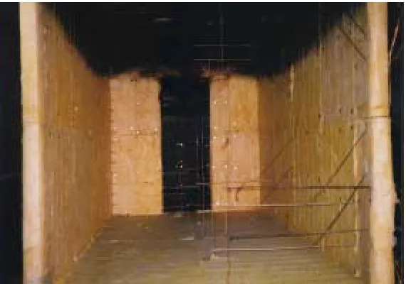
The purpose of this chapter is to describe the configuration of the two compartment experimental set-up used to conduct the fire experiments at McLeans Island for the period 26 November to 1 December 1999. First, a general description is given, followed by specific details on how the two-compartment structure was built.

2.1 General Description

A two-compartment building was constructed to conduct pre-flashover experiments. Starting from steel sections, the frame was built which then allowed Gib® Fyreline and Intermediate Service Board to be placed in the interior of the compartment.

The two compartments were separated by a doorway, which had been constructed from steel studs that were welded to the steel frame. This doorway was then insulated with Gib® Fyreline and Intermediate Service Board, along with the interior of the compartments.

An illustration of the final layout of the two-compartment structure is shown in Figure 2.1 with interior dimensions specified in Table 2.1.

Figure 2.1 Illustration of the Final Layout for the Two-Compartment Structure.

2.4m

800

mm _2.4_m

2.0 m

Fire Room

Adjacent Room

3.6 m 3.6 m

Front Opening

(24)

Table 2.1 Compartment Dimensions

Dimensions Fire Room Doorway Adjacent Room

Height (m) 2.4 2.0 2.4 Length (m) 3.6 0.1 3.6 Width (m) 2.4 0.8 2.4

2.2 Metal Frame

Construction of the two-compartment structure began with a metal frame that was slightly larger than the final interior dimensions. This allowed space for the installation of insulating materials on the inside of the container, so that the final interior dimensions would be met.

The frame was first constructed in two separate sections, and then welded together to form the frame for the two-compartment structure. This formed the starting point for the construction of the two-compartment structure. The frame was elevated 0.5 m to allow access underneath the structure so various instruments could be installed later.

Wooden joists 140 mm × 40 mm were attached to the steel frame at spacings of 600 mm to the horizontal section of the steel frame to provide the foundation for a floor and ceiling.

2.3 Insulation

Once the compartment frame was constructed, the interior was insulated with Gib® Fyreline and Intermediate Service Board to minimize heat transfer and damage to the structure and attached instrumentation.

2.3.1 Gib® Fyreline

(25)

vertical and horizontal centres. The 12.5 mm Gib® Fyreline provides 60 minutes of post-flashover fire protection.

Generous amounts of Gib® 4 Plus was used to seal all joints between Gib® Fyreline plasterboards to ensure minimum leakage within the compartment.

2.3.2 Intermediate Service Board

[image:25.595.156.441.403.603.2]

Upon exposure to temperatures over 100oC (which fire gases exceed considerably), the Gib® Fyreline can dehydrate, altering the thermal properties of the Gib® Fyreline. This undesirable effect would lead to changing thermal properties of the Gib® Fyreline with each experiment. To prevent the dehydration of the Gib® Fyreline from the effects of the fire experiments, Intermediate Service Board (0.6 m × 1.2 m) was fitted to the interior of the compartment, over the Gib® Fyreline (see Figure 2.2 below).

Figure 2.2The Intermediate Service Board used to line the

Interior of the two-compartment structure.

(26)

2.4 Fire Set-up

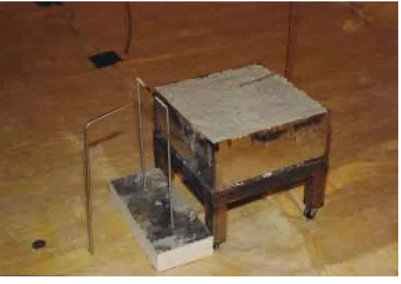
2.4.1 Gas Burner

[image:26.595.155.444.235.440.2]

A square gas burner 300 mm wide, elevated 300 mm above the surface of the compartment floor, was placed in the centre of the fire room to provide the fire (see Figure 2.3 below).

Figure 2.3Gas Burner.

Note: Pilot flame pipe and electrodes to the left of the burner.

A square gas burner is desirable for this experiment as when field models are used to simulate fires, the volume of the compartment is meshed into square and rectangular volumes (see Section 1.3 Zone and Field Models). Therefore a square burner is likely to be modelled more accurately than a circular burner, particularly when a fire is placed in the corner of a room, since a square burner can sit flush in the corner whereas a circular burner cannot.

(27)

the end of a pipe that is expelling combustible gases rapidly is not a buoyancy driven flame, but a momentum driven flame (McCaffery 1995).

The Froude number is a dimensionless number and is determined using the following expression:

r g V Fr

2

= (2.1)

Where: V is the gas velocity (ms-1_),

r is the radius of the orifice (m), and g is the gravitational constant (9.8 ms-1).

To ensure that the LPG from the LPG supply (see Section 2.4.3 for details of the gas supply) is a buoyancy driven flame and not a momentum driven flame, the LPG was dispersed over a much wider area than the diameter of the pipe from the LPG supply that supplies the burner. By feeding the LPG line into the bottom of the burner and dispersing it through a gravel bed of a much larger area, a diffusion flame was established.

2.4.2 Spark and Pilot Flame

A pilot flame was set up to ensure ignition of the burner. The tip of the pilot flame pipe was positioned approximately 150 mm from the fire,at a height of approximately 400 mm. LPG from the main gas source was fed to the pilot flame pipe through the floor.

(28)

2.4.3 Gas Supply

LPG was used to supply the burner and pilot flame for all experiments. Four 45 kg LPG cylinders were stored outside the building and placed on a load cell, enabling the mass loss rate of LPG to be measured during experiments. For all experiments, all the gas cylinders were connected to a single gas line feeding the burner, ensuring consistent gas flow. Gas flow to the burner was controlled by a mass flow meter (see Section 3.6 Mass Flow Meter).

2.5 Fume Hood and Chimney

(29)

3 Instrumentation

The purpose of this chapter is to describe the instrumentation used to measure properties such as temperature profiles, gas species concentrations, and velocities of gas currents generated by the compartmented fires.

3.1 General Description

After the construction of the compartment (the steel frame, Gib® Fyreline, and Intermediate Service Board) was complete, instrumentation was put in place to measure properties of the fires. The physical properties measured were:

• Vertical temperature profiles throughout the compartment, • Surface temperatures throughout the compartment,

• O2, and CO2 concentrations at various locations in the compartment, and • Velocity profiles through the central doorway and exterior opening.

All of these properties are commonly predicted using computer zone or field models (Cox, 1994) to give an approximation of the behaviour of compartmented fires.Thus, instrumentation that measures these properties was placed extensively throughout the compartment.

3.2 Thermocouples

(30)

positions throughout the compartment enabling exposed thermocouples to be corrected for radiation.

3.2.1 Field Trees

To enable the validation of vertical temperature profiles for field models such as SMARTFIRE, thermocouple trees were placed evenly throughout the compartment. Spacing for the nine thermocouple trees is illustrated in Figure 3.1 below.

Figure 3.1Field Tree Positions (Crosses indicate field trees).

The thermocouple trees were positioned 100 mm off the centre of the compartment, with the end 100 mm bent at a 900 angle so that the tip of the thermocouple was positioned along the centre of the room.

Thermocouples used on the trees were type K bare bead 24 gauge with low temperature glass insulation (K24lt), and type K bare bead 24 gauge with high temperature glass insulation (K24ht). Each thermocouple tree held 14 thermocouples (tied in place with wire). Each tree had identical thermocouple spacing, with the exception of the thermocouple tree in the central doorway of the compartment. This had 13 thermocouples spaced evenly at 150 mm, starting at 1900 mm from the floor. Type K24ht were used for the top nine thermocouples for each tree (which were fed into the compartment through the ceiling), as this region undoubtedly reaches high temperatures. The remaining five thermocouples below were of type K24lt (fed through the floor). Spacing for the thermocouples (abbreviated as TC) are listed in

900

mm 1800 mm 2700mm 3600mm 4500mm 5400mm 6300mm 7200mm 150 mm Tree 2 Tree 3 Tree 4 Tree 5 Tree 6 Tree 7 Tree 8 Tree 9 Tree 1

(31)

Table 3.1 Thermocouple Locations on Field Trees

TC Height (mm) 2375 2350 2300 2250 2200 2150 2100

TC Type K24ht K24ht K24ht K24ht K24ht K24ht K24ht

TC Height (mm) 1850 1600 1350 1100 900 600 300

[image:31.595.115.478.195.493.2]

TC Type K24ht K24ht K24lt K24lt K24lt K24lt K24lt

Table 3.2 Thermocouple Locations on Field Trees in the Doorway

TC Height (mm) 1900 1750 1600 1450 1300 1150 1000

TC Type K24ht K24ht K24ht K24ht K24ht K24ht K24ht

TC Height (mm) 850 700 550 400 250 100

TC Type K24ht K24ht K24lt K24lt K24lt K24lt

Figure 3.2Field Thermocouple Trees in the Fire Room.

Note how the thermocouples are bent 900. This is so they are positioned along the centre-line of the room.

Type K24ht and K24lt thermocouples measured temperature as a voltage, which was sent to a computer and converted to a temperature (see Section 3.5 Data Acquisition).

3.2.2 Zone Trees

(32)

[image:32.595.199.397.154.437.2]

(Weaver, 2000) which can then be compared to zone model data) with each thermocouple insulated with stainless steel piping that was mounted to the wall through the exterior of the compartment. Figure 3.3 shows the configuration of the zone thermocouple tree in the adjacent room.

Figure 3.3Zone Tree in the Adjacent Room

3.2.3 Floor and Ceiling Surface Thermocouples

(33)

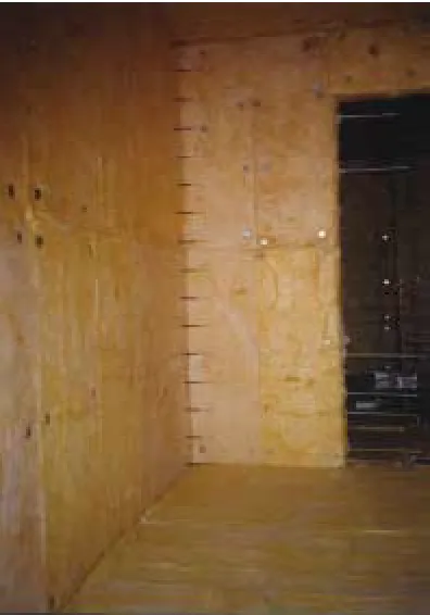
3.2.4 Corner Thermocouples

To measure temperature profiles in the corner (along the centre-line of the compartment) of each room, thermocouples (type K24ht) were positioned in the corners, as shown in Figure 3.4. Thermocouples were positioned in a similar way to the field trees, where they were aligned along the ceiling 100 mm off the centre-line of the compartment, with the end 100 mm bent at a 900 angle so the tip of the thermocouple was positioned along the centre-line of the room. Each corner contained 15 evenly spaced thermocouples. Figure 3.5 shows the spacing for the corner thermocouples. Figure 3.6 shows a picture of the corner thermocouples located near the back wall of the fire compartment.

Figure 3.4Corner Thermocouple Locations

Figure 3.5Corner Thermocouple Positions. Each cross

represents a thermocouple position.

Fire Room 225 Adjacent Room

mm 225 mm

25 mm

75 mm

125mm

175 mm

225 mm

25 mm 75 mm 125 mm 175 mm 225 mm Back

Corner

Front Corner

(34)

Figure 3.6Corner Thermocouples

3.2.5 Aspirated Thermocouples

Radiation can be emitted and absorbed by thermocouples (Blevins, 1999). If the thermocouple’s temperature is high it will radiate heat, lowering its temperature. If a thermocouple is cool but near the fire (for instance, near the floor by the fire) it will absorb radiation, increasing its temperature. Both of these affect the thermocouple’s ability to measure the surrounding air temperature accurately. To overcome this, 20 aspirated thermocouples were positioned throughout the compartment. The aspirated thermocouples were type K24lt thermocouples but insulated with ¼ inch steel tubing. Air is drawn through the steel tubing from a pump. Since the steel pipe conceals the thermocouples, radiation from the fire does not increase its temperature, and emission of radiation by the thermocouple does not reduce its temperature as the constant airflow ensures a very low temperature gradient between the thermocouple and the air.

(35)

Table 3.3 Aspirated Thermocouple Positions

Location Height (mm)

Tree 2 300, 600, 2100, 2250 Tree 4 300, 600, 2100, 2250 Tree 5 300, 600, 1600, 1900 Tree 7 300, 600, 2100, 2250 Tree 9 300, 600, 2100, 2250

Figure 3.7 Aspirated Thermocouples and

Gas Sample Lines

Note: Unfortunately the aspirated thermocouples were not able to be used to correct for the effects of radiation on the bare thermocouples as it was discovered that the pump was drawing insufficient air through the aspirated thermocouple lines.

3.3 Gas Analysis

(36)

Table 3.4 Gas Sampling Point Locations

Position Sampling Point (Height from Floor, mm)

Tree 2 300, 600, 1950, 2250 Tree 4 300, 600, 1950, 2250 Tree 5 400, 700, 1600, 1900 Tree 7 300, 600, 1950, 2250

The gas analysing equipment (referred to as gas analyser throughout the rest of this report) used to determine the concentrations of O2, CO2, and CO consisted of a Servomex 540A paramagnetic oxygen analyser for O2 and a Siemens ULTRAMAT 6.0 NDIR gas analyser (dual-cell, dual beam with a flowing reference gas) for CO2 and CO. Note: The CO concentration for these experiments was below the limitations of the gas analyser, therefore no analysis of CO concentrations for the experiments is given.

(37)

3.4 Bi-directional Probes

Velocity profiles through the doorway and on the ceiling of the compartment were measured using bi-directional probes, as shown in Figure 3.8.

Figure 3.8Bi-directional Probes Located in the Doorway

The 7 bi-directional probes in the doorway were spaced at intervals of 300 mm starting at 100 mm off the floor. The bi-directional probes were then connected to a differential pressure transducer that measured the pressure difference across the bi-directional probe head as a voltage. A computer then recorded this voltage.

By measuring the pressure drop across the bi-directional probe, the velocity can be determined (Emmons, 1995). This is done using the following expression:

ρ

p

(38)

Where: V is the velocity (ms-1),

∆p is the pressure drop across the bi-directional probe (N/m2), and ρ is the density of the air (kg/m3).

Air density is determined using the ideal gas law:

RT Mp

=

ρ (3.2)

Where: M is the molecular mass of the air in the compartment (kg/mol), p is the pressure in the compartment (N/m2),

R is the universal gas constant (8134 J/kg.mol.K), and T is the temperature in Kelvin (K).

The air in the compartment contains combustion products. Since the exact composition of the combustion gasses is not known and 10% of the air or less is used for combustion, the composition is assumed to be ambient air. The molecular weight of air is 28.95 mol/kg at 25oC. Using the ideal gas law the density can be determined:

( )

3

8 . 352

m kg T

=

ρ (3.3)

Therefore, the temperature is required at each bi-directional probe location to determine the density of air. Each bi-directional probes position was in line with type K24lt and type K24ht thermocouples, enabling the temperature at each bi-directional probe to be measured. Note: Unfortunately the bi-directional probe data was unable to be analysed as preliminary results suggested the bi-directional probes contained blockages.

(39)

was used to record temperatures measured by the field, corner and surface thermocouples. All measurements were recorded every 5.2 – 5.3 seconds by both computers and saved as CSV files, which were on average a size of one Mbyte.

3.6 Mass Flow Meter

The mass flow rate of LPG to the burner must be controlled to produce consistent and reproducible fire sizes. To control the mass flow rate of LPG to the burner, a High Flow Mass Controller and Meter Model 5853E was installed between the burner and LPG cylinders. The High Flow Mass Controller and Meter Model 5853E controlled mass flow within the desired range with a quoted error by the manufacturer of 1%.

3.7 Visual Record

(40)

4 Observations

The purpose of this section is to give a qualitative account of the experiments conducted at McLeans Island. The following observations were made:

• As fire size increased, flame height increased.

• All fires hot gases contained soot particles, indicating incomplete combustion. • As fire size increased, so did the level of soot generated by the fire.

• As fire size increased, flame height increased.

• In the fire room, the centrally located fires were all leaning away from the doorway. This behaviour has been observed previously (Quintiere et al., 1981). This is a result of incoming air’s momentum pushing over the fire’s flames.

• As fire size increased, radiation emitted by the fire increased. This was easily felt by standing in front of the compartment.

• The ceiling jet was clearly visible in the adjacent compartment. Since the adjacent compartment had no soffit, this prevented the build-up of hot gases. • In the fire compartment, the production of hot, turbulent gases could be seen.

This increased with an increase in fire size.

• A hot buoyant upper layer could be seen in the fire compartment. This hot upper layer was caused by the soffit constraining gas flow out of the fire compartment.

• The 110 kW corner fire’s flames were the highest of all fires. The corner fire’s flames reached and extended along the ceiling.

(41)

(42)

(43)

(44)

(45)

5 Experimental Results and Discussion

Details relating to measurements made by the field thermocouple trees (commonly referred to as ‘trees’ throughout the rest of this report), corner thermocouples, surface thermocouples, and gas sample lines of the centrally located 55 kW, 110 kW, 160 kW fires, and the 110 kW corner fire are presented and discussed in this chapter.

5.1 Aims

This chapter aims to present steady state results from the data collected by the: 1. Field tree thermocouples,

2. Corner thermocouples, 3. Surface thermocouples, and 4. Gas sampling locations.

Details on how the above four sets of results are expressed, are discussed in Data Presentation and Analysis below.

5.2 Data Presentation and Analysis

This section discusses how data collected for the field trees (see Appendix 1 for tabulated results), corner thermocouples, surface thermocouples (see Appendix 2 for tabulated results), and gas sampling locations are presented and analysed.

5.2.1 Field Trees:

1. Temperature profiles of the field trees are compared for the four fires.

(46)

2. Investigate the temperature variation from the average temperature

during steady state for the thermocouple locations on each tree. This is

expressed on 9 bar graphs (with the four fires represented in each graph) where the standard deviation from the average temperature for each thermocouple tree during steady state, was recorded. The level and location of turbulence and/or mixing of ambient air with hot fire gases inside the compartment will be seen if the standard deviation during steady state is sizeable.

3. An overall comparison per fire between field trees in each room. This

is expressed as 8 Temperature vs. Height scatter graphs with the field trees for each room on one graph, for each fire (Note: Trees 1, 2, 3 and 4 are in the fire room and trees 6, 7, 8, and 9 are in the adjacent room, with tree 5 situated in the doorway. See Section 3.2.1 for locations). This will give an insight to how vertical temperature profiles change within each room.

The average temperatures measured by the corner thermocouples located in the rear and front of the fire room, and in the adjacent room, are presented in tabular format. Each table represents one corner thermocouple set for each fire. The standard deviations for the temperatures measured over the steady state period are included to give an indication of the temperature variations for the thermocouples.

5.2.3 Surface Thermocouples:

The temperatures measured by the surface thermocouples are presented in four separate graphs. They are:

1. Temperature vs. Floor Thermocouple Location, 2. Temperature vs. Ceiling Thermocouple Location,

(47)

These graphs are presented to gain an insight into temperature profiles by the surface thermocouples.

5.2.4 Gas Analysis

The concentration profiles of O2 and CO2 are presented in tabular format where the concentrations for each species at each sample point location for the trees which have sampling lines attached (see Section 3.3 for locations) are presented for the four fires. Included is the ratio of O2 consumption to CO2 production (see Appendix 4 for the background theory on the expected ratio of O2 consumption to CO2 production). This will give an indication of the efficiency of the LPG combustion within the compartment.

5.3 Method

5.3.1 General Method for the Field Trees, Corner Thermocouples and Surface Thermocouples

(48)

presented in Appendix 1. Note: The 110 kW corner fire is denoted as 110 kW c in all graph legends and in some tables throughout the rest of this report).

5.3.2 Method for Field Trees

Reduction Technique for Temperature Profile of the Field Trees for Different Fires

Thermocouple temperatures on each tree were averaged using the method mentioned in Section 5.3.1. One scatter graph is plotted for each field tree, illustrating its vertical temperature profile. Temperatures measured by each tree for the four fires, are represented on each graph.

Reduction Technique for the Variation in Temperature for the Field Trees during Steady State

The standard deviation for the 10 minute steady state period, was determined for the temperatures measured by the thermocouples on each tree, and then plotted on a bar graph. The horizontal axis represents the standard deviation for the temperature on each field tree, and the vertical axis represents the thermocouple height on each tree.

Comparisons Between Field Trees in Each Room per Fire

Thermocouple temperatures on each tree were averaged using the method mentioned in Section 5.3.1. Vertical temperature profiles for trees in each room are plotted on scatter graphs for the four fires.

(49)

5.3.4 Surface Temperature Profiles

Temperature profiles for the surface thermocouples, both ceiling and floor, have been determined in a similar fashion to the tree thermocouples, that is, temperatures recorded were averaged over a ten minute period starting from the 45th minute into the experiments. Throughout this section, surface thermocouples on the ceiling and floor are referred to as ‘ceiling and floor thermocouples’.

5.3.5 Gas Analysis

Concentration profiles of O2 and CO2 were measured at various heights and locations (mentioned in Section 3.3) in the two-compartment structure.

During each experiment, sample point locations were sampled for three minutes, starting from the 13th minute of each experiment. To allow for the time lag associated with sampling lines, the concentration for each sample point location was determined by averaging measurements over the last minute. This gave each sample point two minutes for the gas species at that location to reach the gas analyser.

(50)

5.4 Results

5.4.1 Field Trees

Temperature Profiles of Each Tree for Different Fires

Results for the temperature profiles of each tree for the four fires are listed below in Figures 5.1 – 5.9. Field trees are listed in numerical order.

0 500 1000 1500 2000 2500

0 50 100 150 200 250 300 350

Temperature (oC)

H

e

ight

(

m

)

55 kW 110 kW 160 kW 110 kW c

(51)

0 500 1000 1500 2000 2500

0 50 100 150 200 250 300 350

H

e

ight

(

m

)

55 kW 110 kW 160 kW 110 kW c

Figure 5.2 Temperature Profiles for Tree 2 (All Fires)

0 500 1000 1500 2000 2500

0 100 200 300 400 500 600

H

e

ight (m

m

)

55 kW 110 kW 160 kW

(52)

0 500 1000 1500 2000 2500

0 50 100 150 200 250 300

H

e

ight

(

m

)

55 kW 110 kW 160 kW 110 kW c

0 400 800 1200 1600 2000

0 50 100 150 200 250 300

H

e

ight

(

m

)

55 kW 110 kW 160 kW 110 kW c

(53)

0 500 1000 1500 2000 2500

0 50 100 150 200 250

H

e

ight

(

m

)

55 kW 110 kW 160 kW 110 kW c

0 500 1000 1500 2000 2500

0 50 100 150 200

H

e

ight

(

m

)

55 kW 110 kW 160 kW 110 kW c

(54)

0 500 1000 1500 2000 2500

0 50 100 150 200

H

e

ight (mm)

55 kW 110 kW 160 kW 110 kW c

0 500 1000 1500 2000 2500

0 50 100 150

H

e

ight

(

m

)

55 kW 110 kW 160 kW 110 kW c

(55)

Variation in Temperature for Each Tree

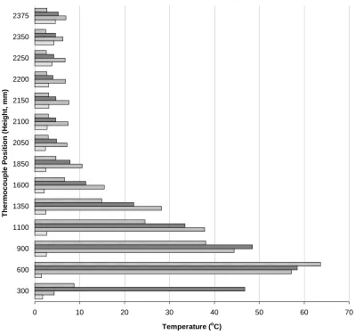
Results for temperature variations (expressed as standard deviations) recorded over the 10 minute steady state period are listed below in Figures 5.10 – 5.18. Field trees are listed in numerical order.

0 2 4 6 8 10 12 14

2375

2350

2250

2200

2150

2100

2050

1850

1600

1350

1100

900

600

300

Ther

m

o

couple P

o

sition (H

eight fr

om

Floor

, m

m

)

55 kW 110 kW 160 kW 110 kW c

(56)

0 2 4 6 8 10 2375

2350

2250

2200

2150

2100

2050

1850

1600

1350

1100

900

600

300

The

rm

oc

ouple

Pos

ition (H

e

ight fr

om

Floor

, m

m

)

55 kW 110 kW 160 kW 110 kW c

(57)

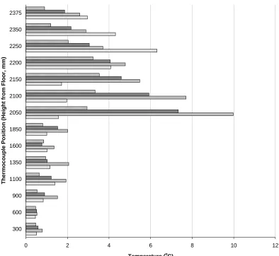
0 10 20 30 40 50 60 70 2375

2350

2250

2200

2150

2100

2050

1850

1600

1350

1100

900

600

300

Ther

m

o

coupl

e P

o

si

ti

on (H

ei

ght,

m

)

[image:57.595.101.500.70.446.2]

55 kW 110 kW 160 kW 110 kW c

(58)

0 2 4 6 8 2375

2350

2250

2200

2150

2100

2050

1850

1600

1350

1100

900

600

300

Thermocouple Position (Height from Floor, mm)

[image:58.595.104.497.73.434.2]

55 kW 110 kW 160 kW 110 kW c

(59)

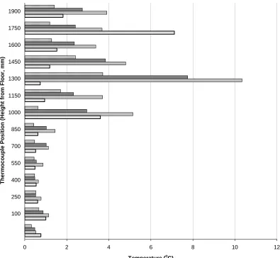
0 2 4 6 8 10 12 1900

1750

1600

1450

1300

1150

1000

850

700

550

400

250

100

The

rm

o

c

ouple

Pos

it

ion (

H

e

ight

f

rom

Floor

, m

m

)

[image:59.595.103.498.72.436.2]

55 kW 110 kW 160 kW 110 kW c

(60)

0 2 4 6 8 10 12 2375

2350

2250

2200

2150

2100

2050

1850

1600

1350

1100

900

600

300

The

rm

oc

ouple

Pos

ition (H

e

ight fr

om

Floor

, m

m

)

[image:60.595.104.498.72.434.2]

55 kW 110 kW 160 kW 110 kW c

(61)

0 2 4 6

2375

2350

2250

2200

2150

2100

2050

1850

1600

1350

1100

900

600

300

Thermocouple Position (Height from Floor, mm)

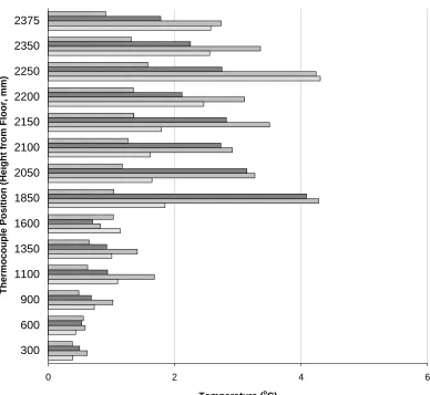
[image:61.595.110.498.73.430.2]

60 kW 120 kW 180 kW 120 kW c

(62)

0 1 2 3 4 2375

2350

2250

2200

2150

2100

2050

1850

1600

1350

1100

900

600

300

T

hermocouple Posit

ion (Height

f

rom F

loor,

m

Temperature (oC)

[image:62.595.115.498.70.421.2]

55 kW 110 kW 160 kW 110 kW c

(63)

0 1 2 3 4 2375

2350

2250

2200

2150

2100

2050

1850

1600

1350

1100

900

600

300

The

rm

oc

ouple

Pos

ition (H

e

ight fr

om

Floor

, m

m

)

55 kW 110 kW 160 kW 110 kW c

[image:63.595.103.501.87.447.2]

(64)

Comparisons between Field Trees in Each Room per Fire

Comparisons between field trees in each room for each fire are listed below in Figures 5.19 – 5.26. Graphs are presented in order of increasing fire size.

0 500 1000 1500 2000 2500

0 20 40 60 80 100 120 140

H

e

ight

(

m

)

[image:64.595.103.493.165.436.2]

Tree1 Tree2 Tree4

(65)

0 500 1000 1500 2000 2500

0 20 40 60 80 100 120

H

e

ight

(

m

)

[image:65.595.103.498.77.343.2]

Tree 6 Tree 7 Tree 8 Tree9

(66)

0 500 1000 1500 2000 2500

0 50 100 150 200 250

H

e

ight

(

m

)

[image:66.595.108.496.101.370.2]

Tree1 Tree2 Tree4

Figure 5.21 Temperature Profiles for the Fire Room, 110 kW Fire

0 500 1000 1500 2000 2500

0 50 100 150 200

Hei

ght

(

m

)

[image:66.595.101.495.422.689.2]

(67)

0 500 1000 1500 2000 2500

0 50 100 150 200 250 300

H

e

ight

(

m

)

[image:67.595.103.496.78.348.2]

Tree1 Tree2 Tree4

Figure 5.23 Temperature Profiles for the Fire Room, 160 kW Fire

0 500 1000 1500 2000 2500

0 50 100 150 200 250

H

e

ight (mm)

[image:67.595.101.495.399.673.2]

(68)

0 500 1000 1500 2000 2500

0 50 100 150 200 250 300 350

H

e

ight

(

m

)

[image:68.595.100.496.78.346.2]

Tree1 Tree2 Tree3 Tree4

Figure 5.25 Temperature Profiles for the Fire Room, 110 kW Corner Fire

0 500 1000 1500 2000 2500

0 50 100 150 200 250

H

e

ight

(

m

)

[image:68.595.100.493.397.668.2]

(69)

Results of the temperature profiles for the corner thermocouples are presented below for the four fires in Tables 5.1 – 5.24.

Table 5.1 Fire Room Rear Corner Temperatures (oC) for the 55 kW Fire Distance from Wall Distance

from Ceiling 25 mm 75 mm 125 mm 175 mm 225 mm

25 mm 126.9 131.0 130.4 130.1 131.2 75 mm 129.3 132.0 131.4 130.9

125 mm 130.0 133.0 131.8 175 mm 130.7 132.5

225 mm 132.4

Table 5.2 Fire Room Rear Corner Temperature Standard Deviations (oC) for the 55 kW Fire Distance from Wall

Distance

25 mm 0.88 0.81 0.71 0.60 0.72 75 mm 0.82 0.70 0.71 0.59 125 mm 0.74 0.72 0.66

175 mm 0.68 0.75

225 mm 0.72

Table 5.3 Fire Room Front Corner Temperatures (oC) for the 55 kW Fire Distance from Wall Distance

25 mm

124.0 122.6 118.0 117.9 122.3

75 mm

122.7 123.2 117.8 122.5

125 mm

125.4 118.0 118.0

175 mm

122.9 118.2

(70)

Table 5.4 Fire Room Front Corner Temperature Standard Deviations (oC) for the 55 kW Fire Distance from Wall

Distance

25 mm

1.03 1.01 1.20 1.41 1.59

75 mm _{1.27 1.31 1.55 1.53} 125 mm _{1.35 1.36 1.50}

175 mm _{1.38 1.27}

225 mm _1.37

Table 5.5 Adjacent Room Corner Temperatures (oC) for the 55 kW Fire Distance from Wall Distance

25 mm _{101.7 102.2 102.5 106.0 105.2} 75 mm _{103.0 103.4 102.1 102.2}

125 mm

102.6 100.5 90.1

175 mm

102.2 98.5

225 mm

101.5

Table 5.6 Adjacent Room Corner Temperature Standard Deviations (oC) for the 55 kW Fire Distance from Wall

Distance

25 mm

1.64 1.59 1.59 1.75 1.60

75 mm _{1.64 1.67 1.55 1.79} 125 mm _{1.65 1.54 1.49}

175 mm _{1.54 1.41}

(71)

Table 5.7 Fire Room Rear Corner Temperatures (oC) for the 110 kW Fire Distance from Wall Distance

25 mm

192.6 198.4 197.3 197.4 200.2

75 mm _{196.5 199.2 200.5 199.4} 125 mm _{197.3 200.5 201.3}

175 mm _{198.0 200.0}

225 mm _200.0

Distance

25 mm _{1.77 1.57 1.30 1.21 1.68} 75 mm _{1.56 1.48 1.63 1.33} 125 mm

1.31 1.44 1.50

175 mm

1.36 1.31

225 mm

1.30

Table 5.9 Fire Room Front Corner Temperatures (oC) for the 110 kW Fire Distance from Wall Distance

25 mm

186.4 186.4 178.0 178.1 186.9

75 mm _{187.0 187.6 178.5 187.0} 125 mm _{190.3 178.5 178.6}

175 mm _{187.4 178.8}

(72)

Table 5.10 Fire Room Front Corner Temperature Standard Deviations (oC) for the 110 kW Fire Distance from Wall

Distance

25 mm

2.16 2.26 2.51 2.92 3.45

75 mm _{2.76 2.82 3.19 3.13} 125 mm _{2.92 2.85 2.93}

175 mm _{2.87 2.70}

225 mm _2.91

Table 5.11 Adjacent Room Corner Temperatures (oC) for the 110 kW Fire Distance from Wall Distance

25 mm _{155.1 156.0 156.2 161.7 162.3} 75 mm _{157.1 158.8 158.0 158.1}

125 mm

157.3 154.3 125.5

175 mm

156.6 150.4

225 mm

155.7

Table 5.12 Adjacent Room Corner Temperature Standard Deviations (oC) for the 110 kW Fire Distance from Wall

Distance

25 mm

2.87 2.73 2.66 3.23 3.01

75 mm _{3.05 3.02 2.82 3.04} 125 mm _{2.96 2.77 2.26}

175 mm _{2.93 2.66}

(73)

Table 5.13 Fire Room Rear Corner Temperatures (oC) for the 160 kW Fire Distance from Wall

Distance

25 mm

241.3 249.0 246.8 248.3 252.3

75 mm _{247.6 250.1 253.2 251.5} 125 mm _{249.0 252.0 253.9}

175 mm _{250.6 251.6}

225 mm _252.1

Distance

25 mm _{2.86 2.78 2.04 2.14 2.81} 75 mm _{2.75 2.64 2.72 2.55} 125 mm

2.63 2.61 2.76

175 mm

2.65 2.43

225 mm

2.62

Table 5.15 Fire Room Front Corner Temperatures (oC) for the 160 kW Fire Distance from Wall

Distance

25 mm

237.8 238.1 230.3 230.0 238.5

75 mm _{239.0 239.5 230.5 238.7} 125 mm _{242.5 230.4 230.5}

175 mm _{239.8 230.6}

An Analysis of Pre Flashover Fire Experiments with Field Modelling Comparisons

An Analysis of Pre-Flashover

Fire Experiments with Field

Modelling Comparisons

Christian van

der

Pump

Fire Engineering Research Report 2000/10

An Analysis of Pre-Flashover Fire

Experiments with Field Modelling

Comparisons

By

Christian van

der

Pump

Supervised by

Dr Charles Fleischmann

Fire Engineering Research Report

March 2000

Abstract

Acknowledgements

Table of Contents

List of Figures

List of Tables

1 Introduction

1.1 Overview

1.2 Experiments

1.3 Zone and Field Models

1.4 Grounds for the Research

1.5 Goals of the Research

1.6 Outline of this Report

1.7 Limitations of this Report

2 Experimental

Set-up

2.1 General Description

2.2 Metal Frame

2.3 Insulation

2.4 Fire Set-up

2.5 Fume Hood and Chimney

3 Instrumentation

3.1 General Description

3.2 Thermocouples

3.3 Gas Analysis

3.4 Bi-directional Probes

( )

3.6 Mass Flow Meter

3.7 Visual Record

4 Observations

5 Experimental Results and Discussion

5.1 Aims

5.2 Data Presentation and Analysis

5.3 Method

5.4 Results