Improved Optimal Power Flow for a Power System
Incorporating Wind Power Generation by Using
Grey Wolf Optimizer Algorithm
Sebaa HADDI, Omrane BOUKETIR, Tarek BOUKTIR
Department of Electrical Engineering, Faculty of Technology, University of Setif, El Bez, 19000 Setif, Algeria [email protected], [email protected], [email protected]
DOI: 10.15598/aeee.v16i4.2883
Abstract. In this paper, an efficient Grey Wolf Opti-mizer (GWO) search algorithm is presented for solving the optimal power flow problem in a power system, en-hanced by wind power plant. The GWO algorithm is based on meta-heuristic method, and it has been proven to give very competitive results in different optimization problems. First, by using the proposed technique, the system independent variables such as the generators’ power outputs as well as the associated dependent vari-ables like the bus voltage magnitudes, transformer tap setting and shunt VAR compensators values are opti-mized to meet the power system operation requirements. The Optimal power flow study is then performed to assess the impact of variable wind power generation on system parameters. Two standard power systems IEEE30 and IEEE57 are used to test and verify the ef-fectiveness of the proposed GWO method. The obtained results are then compared with others given by available optimization methods in the literature. The outcome of the comparison proved the superiority of the GWO al-gorithm over other meta-heuristics techniques such as Modified Differential Evolution (MDE), Enhanced Ge-netic Algorithm (EGA), Particle Swarm Optimization (PSO), Biogeography Based Optimization (BBO), Ar-tificial Bee Algorithm (ABC) and Tree-Seed Algorithm (TSA).
Keywords
Grey Wolf Optimizer (GWO), grey wolves, OPF problem.
1.
Introduction
Optimal power flow problem has been studied for many years and has become one of the most important means
used for adjusting optimal settings of power systems. Therefore, it has received more attention from many researchers throughout the world [1]. Several optimiza-tion techniques have been used to solve this problem, in order to find the optimal solution for operational objective functions in a power system, such as fuel cost, voltage profile and voltage stability enhancement. Some methods are based on nonlinear programming, quadratic programming, Newton techniques and inte-rior point. These methods have many drawbacks, such as high complexity, convergence to local optimum and sensitivity to initial conditions [2].
Intelligent search methods such as meta-heuristic op-timization techniques have been introduced to over-come some optimization problems encountered with classical methods. The most popular ones are; Genetic Algorithm (GA), Particle Swarm Optimization (PSO), Simulated Annealing (SA), Evolutionary Programming (EP), Artificial Bee Colony algorithm (ABC), Ant Colony Optimization (ACO), Differential Evolution (DE). Based on these original methods new derived techniques have been obtained and used in OPF prob-lem as in ABC [3], EGA [4], gradient method and Gen-eral Algebraic Modeling System (GAMS) [5], Efficient Evolutionary Algorithm (EEA) [5], Evolving Ant Di-rection Differential Evolution (EADDE) [6], Differen-tial Search Algorithm (DSA) [7], CSA [8], Krill Herd Algorithm (KHA) [9], Simulated Annealing (SA) [10], Interior Search Algorithm (ISA) [11], Enhanced Ge-netic Algorithm (EGA) [12], BBO [13], PSO [14], Grav-itational Search Algorithm (GSA) [15], Genetic evolv-ing ant direction PSODV hybrid algorithm (PSODV) [16], Real Coded Biogeography-Based Optimization RC-BBO [17] and Evolutionary Algorithm (EA) [18]. Most of these methods are recently extensively used in solving global optimization searching problems and have been giving promising results beside that they
have attractive characteristics, such as easy implemen-tation and fast convergence [18].
A common drawback to meta-heuristic methods is that, in general, the optimization performance is highly dependent on fine parameter tuning. However, the pro-posed approach outperforms these methods in term of convergence speed to the best solution. Moreover, the use of OPF is extended to include the study of renew-able energy systems like wind power, which becomes more and more useful in recent power networks, and many studies are made to integrate this natural power efficiently to a power system. Ranjit and Jadhav in [19], as well as Maskar et al. in [20], presented a study of OPF problem in a system incorporating wind power sources, using modified ABC algorithm named Gbest guided ABC algorithm; the method showed good re-sults for fuel cost optimization case, and voltage profile enhancement, then under wind condition the total op-erating cost is optimized efficiently, compared to other methods. The method presented some benefits con-cerning reserve coefficient adjustment when consider-ing imbalance cost of wind power. Meanwhile, Shanhe et al. [21] presented a new economic dispatch technique based on PSO-GSA algorithm for a power system in-cluding two wind power sources; the method was tested on a six generators’ system connected with two stochas-tic wind power sources. The test yielded good results compared with other results found in the literature with different methods especially for cost and emission reduction. Panda and Tripathy [22], and Mishra and Vignesh [23] introduced another OPF algorithm based on security constrained OPF solution of wind-thermal generation system using modified bacteria foraging al-gorithm. The method was tested on the same system stated in [18], in which the wind power variability was modelled incorporating conventional thermal generat-ing system. Recent works in [19], [24] and [25] pre-sented better results and faster convergence character-istics using Grey Wolf Optimizer algorithm. Grey Wolf Optimizer (GWO) algorithm mimics the behaviour of grey wolves in nature by simulating their leadership hierarchy, through haunting, searching for, encircling, and attacking the prey [26].
The present paper aims to investigate the effi-ciency of GWO algorithm, as a new meta-heuristic population-based algorithm. It presents a solution to the OPF problem of a power system incorporating wind power generation. The rest of the paper is organized as follows; after the introduction, the OPF problem formulation is given in Sec 2. Subsec. 2.2. deals with the OPF problem incorporating wind power. Section 3. presents the GWO algorithm and associ-ated simulation steps for solving the OPF problem. In Sec. 4. simulation results using GWO algorithm are presented and analysed. Section 5. concludes the study.
2.
OPF Problem Formulation
2.1.
Optimal Power Flow
The objective of conventional OPF problem is to min-imize fuel cost for power generation by determining a set of control variables while satisfying system equal-ity and inequalequal-ity constraints. The OPF problem is formulated by [27]:
minf(x, u), (1)
s·tg(x, u) = 0, (2)
h(x, u)≤0, (3)
where [~x]: is the vector of dependent variables consist-ing of slack bus P G1, load bus voltageVL, generator
reactive power outputsQG, and transmission line
load-ingSL. This vector is expressed by:
XT = [PG1, VL1, ..VN D, QG1, ..QGN, Sl1, ..SlN L], (4)
where N D, N G and N L are number of load buses, number of generators, and number of transmission lines, respectively.
[~u] is the vector of independent variables consisting of generator voltagesVG, generator real power outputs
PG except at the slack bus PG1, transformer tap set-tingsTP, shunt VAR compensationQC. This vector is
expressed by:
~
uT=[VG1, ..VN G, .PG2..PGN, TP1, ..TPN T, QC1, ..QCN C],
(5) where: N G, N T, and N C are the number of ther-mal generators, regulating transformers, shunt com-pensators, respectively.
1) Fuel Cost Optimization
The function f from Eq. (1) concerned in the OPF study represents the total generation cost formulation and it is as: f(Pgi) = N G X i=1 aiPgi2 +biPgi+ci ($/h). (6)
When considering valve effect, the functionf; is rewrit-ten as: f(Pgi) = N G P i=1 aiPgi2 +biPgi+ +ci|di(sin(ei(Pgimin−Pgi ($/h), (7)
where: ai, bi, ci, di and ei are fuel cost coefficients of
2) Voltage Profile Improvement
The aim of this objective function is to minimize the load bus voltage deviations from the reference value which is 1 per unit; this function is expressed by:
VD=
NP Q
X
i=1
|Vi−Vref |, (8)
where: VD represents the voltage deviation in (p.u);
Viis theithload bus voltage; andVref is the reference
voltage which is taken here to be 1 p.u, and thus the objective function Eq. (6) becomes as follows:
f(Pgi) = N G P i=1 (aiPgi2 +biPgi+ci)+ +w NP Q P i=1 |Vi−1|, (9)
where: wrepresents a weighting factor selected by the user; many works are choosing w to be 100 in order to keep the variable within the designed limits, as in [1] and [15].The OPF equality constraint such as the active power balance equation is expressed by:
N G
X
i=1
PGi=Pd+Pl, (10)
where: Pd represents the load of the system, andPl is
the total active power loss.
3) OPF Incorporating Inequality Constraints
In order to handle the inequality constraints of depen-dent variables, including slack bus real and reactive power, load bus voltage magnitudes and transmissions line loading; the problem is transformed into uncon-strained OPF problem by penalizing these quantities using the penalty function defined as:
h(xi) = (xi−ximax) ifx > ximax, (ximin−xi)2 ifx < ximax, 0 ifximin≤xi≤ximax. (11)
where: h(xi)is the penalty function of variablexi, here
thexi represents dependent variables,ximinandximax are the upper and lower limits of xi variable,
respec-tively.
The value of the penalty function grows with a quadratic form when the constraints are violated, and equals to zero if the constraints are not violated, while the extended objective function Eq. (6) can be
rewritten as: f(Pgi) = N G P i=1 fi+ηP(Pg1−Pglim1 )2+ηQ(Qg1−Qlimg1)2 +ηV P N L i=1(VLi−PLilim) 2+η S N B P i=1 (Sit−Pitlim)2, (12) where: ηp,ηq,ηv andηsare penalty factors or weights
of active power generation of slack bus, reactive power output of generator buses, PQ bus magnitudes and transmission line loadings respectively. Their values are generally taken to be 100 for the same reason in Eq. (9) [14], [15], [16] and [17].
2.2.
OPF Problem Formulation with
Wind Power
The fuel cost objective in Eq. (6) is augmented with the cost associated with stochastic wind power, as in Eq. (13) [28] FT = N G P i=1 aiPgi2 +biPgi+ci+ +F(Pwj) +Cwj ($/h), (13)
where;F(Pwj)is the cost for generation of wind power
which is directly proportional to the wind power output and is given by:
F(Pwj) =dj×Pwj ($/h), (14)
dj: is the direct cost coefficient of non-utility service,
which equals to zero for the utility services.
Cwj: represents the imbalance cost of investment in
jth wind power source due to two components as in Eq. (15) [29]: Cw= Nw P j=1 (Kp,j×Wj,ue)+ + Nw P j=1 (KR,j×Wj,oe) ($/h), (15)
where: Wj,ue and Wj,oe, are given by the following
expressions: Wj,ue= (Pwr,j−Pwj) exp − vr,jkj ckji −exp − vkjo,j ckji + Pwr,jvin,j vr,j−vin,j +Pwj exp − vkjr,j ckji −exp − vkj1,j ckji + Pwr,jvin,j vr,j−vin,j · ( Γ " 1 + k1 i, vkj1,j ckji kj# −Γ " 1 +k1 i, vkjr,j ckji kj# ) , (16)
Wj,oe= (Pwr,j) 1−exp − vin,jkj ckji −exp − vo,jkj ckji + Pwr,jvin,j vr,j−vin,j +Pwj exp − vr,jkj ckji −exp − vkj1,j ckji + Pwr,jvin,j vr,j−vin,j · ( Γ " 1 + 1 ki, v1kj,j ckji kj# −Γ " 1 + k1 i, vkjr,j ckji kj# ) , (17)
where: v1 = vin,j + (vr,j−vin,j)PW,j/PW r,j; k > 0,
c >0are the shape factor and scale factor, respectively.
PW r; is the available active power for the jth wind
turbine. PW r,j, is the rated wind power output, PW,j
is the actual wind power output of jth wind turbine.
Vin, V0 and Vr are the cut-in, cut-off and rated wind
speed, respectively.
Equation (15) represents the stochastic nature of wind power output for which the following parameters are associated:
• Kp,j: penalty cost coefficient for not using all
available power from jth wind turbine due to under-generation estimated fromjthwind turbine,
• KR,j: reserve cost coefficient due to the reserve
capacity used to compensate the over-estimated wind power ofjth wind turbine.
• Wj,ueandWj,oe, are the expected value ofjthwind
turbine for over-estimated and under-estimated energy output which was calculated using Eq. (16) and Eq. (17) [2].
To deal with wind speed variations of wind turbine, the generated power from wind can be approximated with respect to particular wind speedV, as follows [2]:
Pw(V) = 0 V ≤Vin, aV3+bV2+cV +d V r> V > Vin, Pwe Voff> V ≥Vr, 0 V ≥Voff. (18)
Pw(V) is the available wind power output, a, b, c,
andd; are constants, in this study the generated wind power output is used as negative real power load con-nected at special bus in the test system.
1) System Equality Constraints with Wind Energy
The equality constraints for the case of wind power are expressed by [26]: N G X i=1 PGi+ Nw X j=1 PW j=Pd+P−l. (19)
The active power losses are given by the formula:
Ploss= N l P n=1 Gnij |Vi |2+|Vj |2−2|Vi||Vj | cos(δi−δj)], (20)
where: i and j are the sending and receiving ends of particular linen. N l; is the number of lines. The equal-ity constraints from Eq. (8) and Eq. (9) are rewritten for the wind nodej as:
PW j−Pdj−Pj,cal(V, δ) = 0, (21)
QW j−Qdj−Qj,cal(V, δ) = 0. (22)
The control variables vector is modified as:
~
uT = [VG1, ..VN G, .PG2..PGN, Pw1, ..PNw,
Tp1, ..TpN T, QC1, ..QCN C],
(23) where: NW represents the number of wind generators
in the power system network.
2) Wind Generators Constraints
In addition to the precedent inequality constraints, we can write;
0≤PW i≤PW r,i, i= 1, ..Nw, (24)
where: PW r, is the rated active power output of the
ith wind turbine unit.
3) Spinning Reserve Constraints Model for OPF with Wind Energy
The spinning reserve is the reserve capacity used for sudden load increase, unpredictable fall in wind power output or forced outage of thermal generators units. The spinning reserve has two limits which are the upper and lower limits that represent system up and system down spinning reserves USR and DSR; given by the following expressions: [2] and [30]:
PU S≥RU SR+r%× Nw X j=1 PW,j, (25) PDS≥RDSR×s% +r%× Nw X j=1 PW,j, (26)
where; ris the influence coefficient that gives the per-centage of wind power contributing to USR and DSR. The USR can be represented with respect to the total load and total wind power by:
N
X
i=1
PU Si ≥Pd×s% +r%×PW T, (27)
where: U Si represents the maximum up spinning
re-serve limit of ith thermal unit, and s is the
percent-age of load contributing to USR, these constraints will be considered during the implementation of GWO al-gorithm. As the rate of wind power penetration in-creases, it becomes more difficult to predict the exact amount of power injected by all generators into the power grid. This added more uncertainty when ac-counting the spinning reserve requirements.
3.
Used Algorithm
3.1.
GWO Algorithm
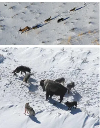
Grey Wolf Optimizer (GWO) is a new algorithm pro-posed by Mirjalili et al. in 2014 [31]. This algorithm mimics the leadership hierarchy and hunting technique used by grey wolves to catch their prey until stopping its movement. GWO is similar to other population-based meta-heuristic algorithms, by simulating the nat-ural behavior of grey wolves in their social life when searching for food; they follow hierarchy structure in the group (Fig. 1). The first level representing the lead-ers of the group is called (alpha), the second level in the hierarchy of grey wolves is (beta) which helps alpha to make decisions. The next levels are delta and omega; they are the lowest ranks in the group; they have to eat after all levels. In fact, these wolves are group-hunting that take three main steps; chasing, encircling and at-tacking. The algorithm starts with a given number of wolves whose positions are randomly generated.
3.2.
Steps of GWO Algorithm
Four types of wolves groups can be used to simulate the leadership hierarchy of grey wolves. This hierarchy is represented in Fig. 1, respecting the social dominant degree, the high class is named alpha (α), mostly re-sponsible for making decisions about hunting and order the other wolves in the pack.
(α) (β) (δ) (ω)
Kappa (κ) and lambda (λ)
Fig. 1: Hierarchy levels of grey wolves.
Fig. 2 a) attacking prey b) hunting prey by wolves (a)
(b)
Fig. 2: (a) attacking prey (b) hunting prey by wolves.
They can be considered as the fittest solution. The next level in the chain is called beta (β), the wolves of this level help the alpha ones in supervising other groups’ actions. They can replace the alpha wolves when they die or become aged and begin to be the best candidate solution. The lowest ranking grey wolves are delta (δ) wolves and omega (ω) wolves [27] and [32]. Therefore types α, β, and δ leading the opti-mization (hunting) process, while ω group is to track them. Kappa (κ) and lambda (λ) wolves are directed by omega in the hierarchy.
The main steps involved in the original GWO algo-rithm are as follows:
• Initialize the search agents.
• Assign Alpha, Beta and Gamma by fitness.
• Encircling the prey: represent the circular area around the best solution (prey). This step can be represented by the following equations:
D=|C·X~p(t)−X(t)|, (28)
X(t+ 1) =|X~p(t)−A·D|, (29)
where: X~p is the prey’s position vector. (A~) and (C~),
are vectors given by the following equations:
a= 2(1−t/Tmax), (30) ~
A= 2·ar1−a, (31)
~
C= 2r2, (32)
where: t is the current iteration andTmax, total itera-tions.
The parameter a decreases linearly in the range of [2,0] for successive iterations using Eq. (30); that model wolfs behaviour approaching the prey;r1andr2 are random vectors in the range[0,1].
• Hunting step: the encircling process comes to the second step involving hunting guided by the alpha wolf group. The following equations represent this step: Dα=|C1·Xα(t)−X(t)|, (33) Dβ=|C2·Xβ(t)−X(t)|, (34) Dδ =|C3·Xδ(t)−X(t)|, (35) X1=Xα−A1·DαX2, (36) X2=Xβ−A2·DβX3, (37) X3=Xδ−A3·Dδ, (38) X(t+ 1) = (x1+X2+X3)/3. (39) • Attacking the prey: Firstly, r1 and r2 are ran-domly selected for mutation (Aand C), then the base vector (X) is randomly selected within the range [r1, r2], that is to drive the algorithm to global solution and avoid local optima. The fact that “a” decreases from 2 to 0 makes the explo-ration more efficient, but slows down the GWO convergence characteristics. So, the final step of attacking the prey is done by decreasing linearly the value of “a” from 2 to 0 [33].
• Steps 2 to 5 are then repeated until the maximum number of iterations is reached.
3.3.
Pseudo Code for GWO
Algorithm
Initializethe grey wolf population; Xi; i=1. . . n
Initializeparameters; a, A, and C
Calculatethe fitness of each Search_Agent; Xa=the best search agent;
Xβ=the second best search agent;
Xδ the third best search agent;
WhileIter≤Max_Iter
Forj∈{search space}
Sort the population of grey wolves according to their fitness
Update the Update the position of the current Search Ahent using Eq. (39);
endfor% search space
Update a, A and C
Calculatethe fitness of the new search agents;
Update Xa ,Xβ andXδ
Iter=Iter+1;
End; Return, Best solution found so farXa;
4.
Case Study and Simulation
Results
In this section, the optimal power flow problem is im-plemented using GWO algorithm and two case stud-ies are considered. For the first case study, the simu-lation is carried out on IEEE30- bus system as used in [34], by solving conventional OPF and consider-ing quadratic model of thermal generators cost usconsider-ing Eq. (6). Then, the OPF problem is implemented con-sidering wind power for a given wind speed and cost profiles. Later, the OPF problem is implemented con-sidering different wind speed profiles.
In the second case study, the simulation is carried out on IEEE57-bus system. The purpose of these studies is to validate the results obtained using GWO algorithm by comparing them with the results available in the literature.
4.1.
Case Study N
◦1: IEEE30 Bus
Test System
1) Case 1.1: OPF with Quadratic Fuel Cost
The objective function for this case study is given by Eq. (6), for all thermal generators units, the numerical data and parameters are taken from [35], the PQ bus voltages are between 0.95 and 1.05 p.u, the shunt Var Compensator are not considered in this case study, ex-cept for the two shunt capacitors banks, at nodes 10
and 24 of 19 and 4.3 Mvars respectively. The optimum control settings obtained by using GWO algorithm are presented in Tab. 1.
Tab. 1: Optimal power flow without considering dependent variables. Control variables Lower/up per limits Case 1.1 Case 1.2 Case 1.3 P1(MW) 50 200 176.1721 176.472 199.988 P2 20 80 48.0926 48.795 20.0000 P5 15 35 21.1376 21.506 15.0152 P8 10 30 23.3591 21.799 10.0000 P11 10 30 11.3591 11.993 10.0000 P13 12 40 12.0000 12.000 12.0000 V1 0.95 - 1.05 1.0600 1.0600 1.06000 V2 0.95 - 1.10 1.0512 1.0512 1.0512 V5 0.95 - 1.10 1.0224 1.0224 1.0224 V8 0.95 - 1.10 1.0333 1.0333 1.0333 V11 0.95 - 1.10 1.0820 1.0820 1.0820 V13 0.95 - 1.10 1.0910 1.0910 1.0910 T11 0.90 - 1.10 1.0150 1.0150 1.0170 T12 0.90 - 1.10 0.9070 0.9070 0.9070 T13 0.90 - 1.10 0.9680 0.9680 0.9680 T14 0.90 - 1.10 0.9550 0.9550 0.9550 Fuel cost $/h -801 .1769 804 .4726 910 .6575 Power loss - 9.1528 9.202 12.709 Voltage deviations - 0.10 0.1082
-In order to assess the potential of the proposed ap-proach, a comparison between the obtained results of fuel cost and those reported in the literature has been carried out. The results of this comparison are given in Tab. 2. It is worth mentioning that the comparison has been carried out with the same test system data.
Different OPF results of active generation powers and losses for different case studies are given in Tab. 1.
50 100 150 200 250 300 350 400 Iteration 798.5 799 799.5 800 800.5 801 801.5
Best fuel cost ($/h)
GWO
Fig. 3: Convergence characteristic of IEEE30 bus system case 1.1.
The best fuel cost calculated by the proposed algo-rithm for this case is 801.1769 $/h, which is better than
Tab. 2: Comparison of quadratic fuel cost case 1.1.
Methods Fuel cost ($/h)
MDE [35] 802.376
ABC [3] 802.305
EGA [4] 802.060
GAMS [5] 801.519
GWO 801.176
that obtained by many other algorithms as depicted in Tab. 2. The corresponding convergence graph is shown in Fig. 3.
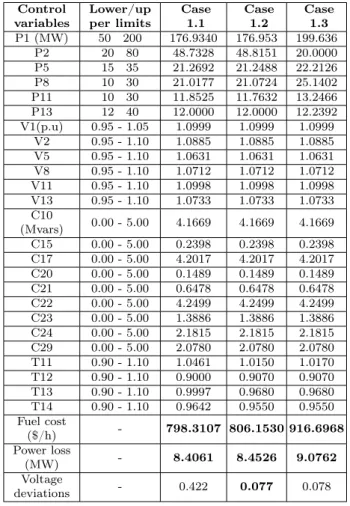
Tab. 3: Optimal power flow considering dependent variables.
Control variables Lower/up per limits Case 1.1 Case 1.2 Case 1.3 P1 (MW) 50 200 176.9340 176.953 199.636 P2 20 80 48.7328 48.8151 20.0000 P5 15 35 21.2692 21.2488 22.2126 P8 10 30 21.0177 21.0724 25.1402 P11 10 30 11.8525 11.7632 13.2466 P13 12 40 12.0000 12.0000 12.2392 V1(p.u) 0.95 - 1.05 1.0999 1.0999 1.0999 V2 0.95 - 1.10 1.0885 1.0885 1.0885 V5 0.95 - 1.10 1.0631 1.0631 1.0631 V8 0.95 - 1.10 1.0712 1.0712 1.0712 V11 0.95 - 1.10 1.0998 1.0998 1.0998 V13 0.95 - 1.10 1.0733 1.0733 1.0733 C10 (Mvars) 0.00 - 5.00 4.1669 4.1669 4.1669 C15 0.00 - 5.00 0.2398 0.2398 0.2398 C17 0.00 - 5.00 4.2017 4.2017 4.2017 C20 0.00 - 5.00 0.1489 0.1489 0.1489 C21 0.00 - 5.00 0.6478 0.6478 0.6478 C22 0.00 - 5.00 4.2499 4.2499 4.2499 C23 0.00 - 5.00 1.3886 1.3886 1.3886 C24 0.00 - 5.00 2.1815 2.1815 2.1815 C29 0.00 - 5.00 2.0780 2.0780 2.0780 T11 0.90 - 1.10 1.0461 1.0150 1.0170 T12 0.90 - 1.10 0.9000 0.9070 0.9070 T13 0.90 - 1.10 0.9997 0.9680 0.9680 T14 0.90 - 1.10 0.9642 0.9550 0.9550 Fuel cost ($/h) - 798.3107 806.1530 916.6968 Power loss (MW) - 8.4061 8.4526 9.0762 Voltage deviations - 0.422 0.077 0.078
For the methods EADDE in [6], GABC in [7], EEA in [5], CSA in [8], KHA in [9], SA in [10], and ISA in [11], the PQ bus voltages are between 0.95 and 1.1 p.u, the transformers tap setting and shunt Var compen-sators are considered in the same case study, and the generator voltages are taken close to their high per-missible limit. Table 3 shows the corresponding op-timal power flow results when using the opop-timal set-tings of dependent variables. It can be observed from Tab. 4 that GWO algorithm gives better results. The system reactive generation powers for this case study are within their specified limits as in Tab. 5. Table 6 presents a comparison of optimal power flow results of the proposed algorithm with other methods found in
Tab. 4: Comparison when optimizing dependent variables.
Methods Fuel cost ($/h)
EADDE [6] 800.204 DSA [7] 800.388 EEA [5] 800.083 CSA [8] 799.707 EGA [12] 799.5600 BBO [13] 799.1116 KHA [9] 799.0310 MFPA [40] 799.1592 GSA [15] 798.675 GWO 798.3107
Tab. 5: Comparison when optimizing dependent variables.
React. Power Gen. Limits Qg
Q1 -20 200 -18.7646 G2 -40 50 23.1157 Q5 -40 40 27.3300 Q8 -15 40 33.7790 Q11 -6 24 17.9905 Q13 -6 24 2.55070
Tab. 6: GWO-OPF results comparison for case 1.1.
Pgi
(MW) SA ISA KHA GSO GWO
P1 173.15 177.124 177.04 174.920 176.9046 P2 48.54 48.933 48.690 44.150 48.7226 P5 19.23 21.3175 21.300 21.760 21.2697 P8 12.81 21.0006 21.080 25.730 21.0509 P11 11.64 11.8605 11.880 11.120 11.8556 P13 12.00 11.860 12.020 13.810 12.0000 Tot. Gn (MW) 277.37 292.095 292.01 291.49 291.8034 Cost ($/h) 799.45 799.277 799.03 799.06 798.3106 Losses (MW) 9.200 8.695 8.610 8.48 8.4034
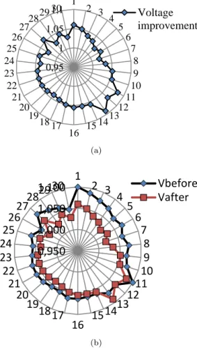
the literature as in [3] and [19]. Figure 6(a) shows the voltage profile of case 1.1, without improvement.
2) Case 1.2: OPF with Voltage Profile Improvement
Minimizing only the total fuel cost using OPF problem as in case 1.1; can result in a feasible solution, but voltage profile may not be acceptable. Thus, in this second case, the objective here is to minimize the fuel cost and improving the voltage profile at the same time by minimizing the voltage deviation of PQ buses from the unity 1.0. [36].
The results obtained using the proposed approach are compared with other methods in the literature as shown in Tab. 7 where the total cost found by GWO, in this case, is better than that obtained before.
Figure 4 shows the convergence graph. Figure 5 presents the transmission load flow of the system, from this figure, we can see that the obtained transmission
Tab. 7: Comparison when optimizing dependent variables.
Methods Fuel cost ($/h)
BBO [13] 804.998 PSO [14] 806.380
DE [1] 805.262
GWO 806.1530
loading amounts are within acceptable limits. As we can see from Fig. 6(a), the voltage magnitude is en-hanced after the improvement by GWO, and all the load bus voltages are within the permissible range.
100 200 300 400 500 600 700 Iteration 803 803.5 804 804.5 805 805.5 806
Best fuel cost ($/h)
GWO
Fig. 4: Convergence characteristic of IEEE30 bus system case 1.2. 0 10 20 30 40 50 line number 0 20 40 60 80 100 120 140 load flow (MW) Normal case Load flow limits
Fig. 5: Transmission Load flows obtained by GWO.
3) Case 1.3: OPF for Fuel Cost Including Valve Point Effect
Considering the same system data as in [23], the valve point effect is incorporated and the fuel cost is evalu-ated using the Eq. (7). Simulation of power flow results
0,95 1 1,05 1,1 1 2 3 4 5 6 7 8 9 10 11 12 13 14 15 16 17 18 19 20 21 22 23 24 25 26 2728 29 30
Voltage
improvement
(a)0,950
1,000
1,050
1,100
1
2 3
4
5
6
7
8
9
10
11
12
13
14
15
16
17
18
19
20
21
22
23
24
25
26
27
28
2930
Vbefore
Vafter
(b)Fig. 6: a) Bus voltage magnitude case 1.2, b) Comparison of voltage profile of IEEE30 bus case 1.1 & case 1.2.
of this case study is compared with other available re-sults as in Tab. 8.
Tab. 8: Obtained results comparison case 1.3.
Methods Fuel cost ($/h)
PSO [14] 932.7642 ABC [3] 945.4495 GSA [15] 929.7240 GABC [19] 931.7450 BBO [13] 919.7647 MFPA [40] 917.8298 GWO 916.6968
4) Case 1.4: System Analysis Under (N-1) Contingency
To investigate the efficiency of GWO under contin-gency, a line outage conditions are created on the test system as in [23], in which four contingency conditions are considered (lines: 12–15, 10–20, 15–23 and 6–28). For these four conditions, the voltage profile for nor-mal and contingency conditions is shown in Fig. 7, and corresponding load flow profile is in Fig. 8.
0,80 0,90 1,00 1,10 1 2 3 4 5 6 7 8 9 10 11 12 13 14 15 16 17 18 19 20 21 22 23 24 25 26 27 28 29 normal_case
Fig. 7: Voltage profile for normal and contingency conditions.
0 10 20 30 40 50 line number 0 20 40 60 80 100 120
active load flow (MW)
load flow for normal conditions LF for contengency conditions
Fig. 8: Load flow profile for normal and contingency conditions.
The load-bus voltages of contingency case are below their normal limit (deviated from their normal lim-its).To alleviate this problem we apply Eq. (11) and Eq. (12), to bring the voltage at these load buses within 0.95 and 1.05 p.u. Figure 9 shows the corrected voltage profile.
4.2.
Case 2: OPF with Wind Energy
Case Study
1) Case 2.1: OPF with Stochastic Wind Power Modelling
In this section, GWO algorithm is used to solve OPF problem for system including stochastic wind power in addition to conventional thermal generators. In this case, the system has been modified by replacing con-ventional generators by wind farms located at buses 5, 11 and 13; each with a total capacity of 60 MW. Two case studies are considered here: in the first case, the wind power is modelled using Weibull distribution
0 5 10 15 20 25 30 Bus number 0.8 0.85 0.9 0.95 1 1.05 1.1 1.15 1.2
Voltage magnitude (p.u)
voltage profile during contengency Voltage profile after correction
Fig. 9: Voltage profile for normal and contingency conditions.
function in form of imbalance costs of wind power in the main cost objective Eq. (15), which is minimized subject to all given constraints. While, in the second case study, the OPF problem is solved considering dif-ferent wind speeds.
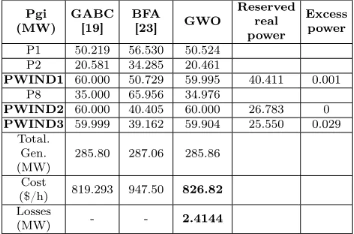
The test system data given in [23] are taken for this study. The simulation convergence curve and voltage at different buses of the system are given in Fig. 10 and Fig. 11, OPF schedule is given in Tab. 9; the optimal results are then compared with GABC [19] and BFA [23]. 20 40 60 80 100 120 140 160 180 200 Iteration 840 860 880 900 920 940 960
Best fuel cost ($/h)
GWO
Fig. 10: Convergence graph of fuel cost for wind case.
The obtained results show that the GWO method performs better when compared with other methods for the same case study. The reserved power is higher than the surplus power in Tab. 9, which justifies the fact that the utility service is to purchase an important amount of reserve for covering any unavailable wind energy.
0,95
1,00
1,05
1,10
1
2 3
4
5
6
7
8
9
10
11
12
13
14
15
16
17
18
19
20
21
22
23
24
25
26
27
28
2930
Vwind
Fig. 11: Bus voltage magnitude for wind case.
Tab. 9: Simulation results for wind case study.
Pgi (MW) GABC [19] BFA [23] GWO Reserved real power Excess power P1 50.219 56.530 50.524 P2 20.581 34.285 20.461 PWIND1 60.000 50.729 59.995 40.411 0.001 P8 35.000 65.956 34.976 PWIND2 60.000 40.405 60.000 26.783 0 PWIND3 59.999 39.162 59.904 25.550 0.029 Total. Gen. (MW) 285.80 287.06 285.86 Cost ($/h) 819.293 947.50 826.82 Losses (MW) - - 2.4144
As seen from Fig. 10, the total fuel cost is decreased by the integration of wind power source in the system.
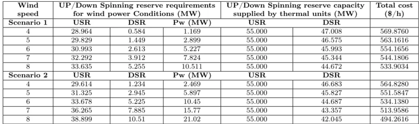
2) Case 2.2: OPF Study with Wind Energy Considering Reserve Constraints
Case 2.2.1: OPF without Wind Power
In this case study, we used the same configuration as in [2], by considering the nodes 1, 2, 13, 22, 23 and 27 as generator buses and total system load of 189.2 MW. First, we proceeded for optimal power flow without wind energy; the simulation results of this case are compared to those reported in [2], as shown in Tab. 10. It can be noticed that the obtained GWO cost is better comparing with the case without wind power. Case 2.2.2: Wind Energy with Zero Cost
Two scenarios of wind power integration levels are con-sidered in this study; 10 %, and 20 % of the system load. These levels are connected to bus 8. Using Eq. (25), Eq. (26) and Eq. (27), we calculated the spin-ning reserve under different wind speeds at the second hour, assuming the wind speed at the first hour was 3 m·s−1.
Tab. 10: Simulation results for wind case with spinning reserve.
Wind UP/Down Spinning reserve requirements UP/Down Spinning reserve capacity Total cost speed for wind power Conditions (MW) supplied by thermal units (MW) ($/h)
Scenario 1 USR DSR Pw (MW) USR DSR
4 28.964 0.584 1.169 55.000 47.008 569.8760
5 29.829 1.449 2.899 55.000 46.575 563.1616
6 30.993 2.613 5.227 55.000 45.993 554.1656
7 32.292 3.912 7.824 55.000 45.344 544.1806
8 33.635 5.255 10.511 55.000 44.672 533.9034
Scenario 2 USR DSR Pw (MW) USR DSR
4 29.614 1.234 2.469 55.000 46.683 564.8280 5 31.325 2.945 5.897 55.000 45.827 551.5847 6 33.678 5.225 10.45 55.000 44.687 534.1380 7 36.265 7.885 15.77 55.000 43.357 513.9586 8 38.899 10.51 21.02 55.000 42.045 494.2616
0,9
0,95
1
1,05
1,1
1
2 3
4
5
6
7
8
9
10
11
12
13
14
15
16
17
18
19
20
21
22
23
24
25
26
27
2829
30
Bus voltage
Fig. 12: Voltage profile at different nodes for modified system.
Tab. 11: OPF results of modified IEEE30 bus system.
Pgi (MW) GWO Without wind EPSO [2]
P1 43.4397 43.425 P2 57.7903 55.785 P13 17.4824 17.716 P22 23.0944 23.131 P22 17.2086 18.241 P27 32.6450 33.307 W1 - -Total gen. (MW) 191.6604 191.605 Cost ($/h) 574.7271 574.766 Losses (MW) 2.4604 2.408 Voltage div 1.0572
The spinning reserve of the system wass= 15% of the total demand, and the up-spinning reserve was set to improve the safety of the power system operation under wind intermittent conditions or uncertain wind power. Simulation results for wind case study.
This was achieved by using Eq. (27), in which this reserve constraint of wind generation was r= 50% of the system load. After computing the wind power us-ing Eq. (25), we run the OPF program to calculate the cost associated with this wind injection then we pro-ceeded to the calculation of different spinning reserve constraint limits, the obtained results are depicted in Tab. 10.
The wind speeds values were respectively 4, 5, 6, 7, and 8 m·s−1; different computation results of scenarios 1 and 2 are presented in Tab. 12 and the system voltage profile is shown in Fig. 13.
Tab. 12: Simulation results for wind case study. Wind
speed (m·s−1)
4 5 6 7 8
Scenario 1(10 % of wind penetration)
Cost
($/h) 571.24 571.565 581.487 605.395 644.38
Scenario 2 (20 % of wind penetration)
Cost
($/h) 570.92 586.359 643.340 762.651 936.10
Case 2.2.3: OPF Considering Wind Power Cost
In this case, we assume that the wind power has the same direct cost of [19]d1= 1$/h, without considering the imbalance cost. Simulation results for wind case study.
The simulation result is shown in Tab. 12, we can see that when wind speed increases, the total operation cost increases too, due to the wind direct cost impact on the total operating cost.
4.3.
Case 3: OPF with Stochastic
Wind Speed
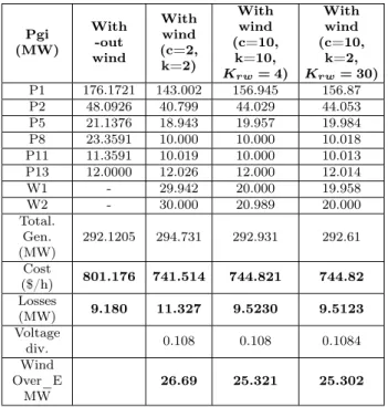
In this case study and in order to check the effect of uncertain wind power on the test power system, two wind farms each with capacity of 30 MW have been connected at two separate locations; at nodes 26 and node 30 as in [19]. The results obtained are then com-pared with the case without wind energy.
Two cases are considered here; the first one where the scale factor “c” takes the values of 3 to 30 while keeping the shape factor at k = 2, then by keeping the scale factor constant at the value 10 and varying the reserve coefficient (Krw) from its base value of 4,
and with the installed wind power capacity for each wind farm of 20 MW instead of 30 MW by applying the proposed approach taking into consideration these conditions, we find the results as shown in Fig. 13(a).
For the second case study, we maintained the val-ues of wind turbines Weibull model factors constant,
vin= 4 m·s−1,vr= 12m·s−1,vout= 25m·s−1,c= 3,
k = 2, Kpw = 1, Krw = 4, but considering the direct
costs of the two wind farmsd1 =d2 = 1.3 $/h. Simu-lation results are presented in Tab. 13, the convergence characteristics for different values of reserve coefficient “Krw” is given in Fig. 13(b).
Generally, the direct cost of wind power is less than the average cost of thermal power, and the penalty cost of not using all the available wind power is consid-ered less than the direct cost. From Fig. 13(b), it can
10 20 30 40 50 Iteration 745 745.5 746 746.5 747 747.5
operating fuel cost ($/h)
Krw=4 Krw=10 Krw=20 Krw=30 Krw=40 (a) 50 100 150 200 250 300 350 400 Iterations 750 755 760 765 770 775 780 785 total cost ($/h) GWO c=4 c=10 c=20 c=30 (b)
Fig. 13: Convergence characteristic for a) different values of re-serve coefficient (Krw), b) different values of scale
fac-tor “c”.
Tab. 13: Simulation results for wind case study.
Pgi (MW) With -out wind With wind (c=2, k=2) With wind (c=10, k=10, Krw= 4) With wind (c=10, k=2, Krw= 30) P1 176.1721 143.002 156.945 156.87 P2 48.0926 40.799 44.029 44.053 P5 21.1376 18.943 19.957 19.984 P8 23.3591 10.000 10.000 10.018 P11 11.3591 10.019 10.000 10.013 P13 12.0000 12.026 12.000 12.014 W1 - 29.942 20.000 19.958 W2 - 30.000 20.989 20.000 Total. Gen. (MW) 292.1205 294.731 292.931 292.61 Cost ($/h) 801.176 741.514 744.821 744.82 Losses (MW) 9.180 11.327 9.5230 9.5123 Voltage div. 0.108 0.108 0.1084 Wind Over_E MW 26.69 25.321 25.302
be seen that, the larger the value of c the higher the value of wind speed and hence wind power penetration amount. However, the amount of wind power injected at bus 26 remains, less than that injected at bus 30, due to the thermal loading limit of the transmission line at this section.
4.4.
Case Study N
◦2: IEEE57 Bus
Test System
This system consists of 7 thermal generators, with bus 1 is considered as slack bus; 2, 3, 6, 8, 9 and 12 as PV buses, 50 load buses and 80 lines, among which 17 lines are equipped with tap changing transformers. In addition, three shunt Var compensators are installed at buses 18, 25 and 53. The system data are taken from [37]. Two cases are investigated in this case study:
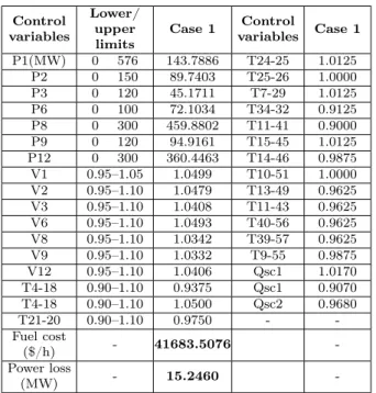
1) Case 1: OPF for Quadratic Fuel Cost
In this case study, the objective function to be opti-mized is represented by the quadratic fuel cost, related to thermal generators unit described by the Eq. (6).
The optimal power flow for the first case study us-ing GWO takes the settus-ings of the algorithm as the followings: search agent number equals to 30, and the number of runs equals to 300. These are the same system settings used for the other methods, and the obtained simulation results are shown in Tab. 14.
Tab. 14: Optimal control variables settings for case 1. Control variables Lower/ upper limits Case 1 Control variables Case 1 P1(MW) 0 576 143.7886 T24-25 1.0125 P2 0 150 89.7403 T25-26 1.0000 P3 0 120 45.1711 T7-29 1.0125 P6 0 100 72.1034 T34-32 0.9125 P8 0 300 459.8802 T11-41 0.9000 P9 0 120 94.9161 T15-45 1.0125 P12 0 300 360.4463 T14-46 0.9875 V1 0.95–1.05 1.0499 T10-51 1.0000 V2 0.95–1.10 1.0479 T13-49 0.9625 V3 0.95–1.10 1.0408 T11-43 0.9625 V6 0.95–1.10 1.0493 T40-56 0.9625 V8 0.95–1.10 1.0342 T39-57 0.9625 V9 0.95–1.10 1.0332 T9-55 0.9875 V12 0.95–1.10 1.0406 Qsc1 1.0170 T4-18 0.90–1.10 0.9375 Qsc1 0.9070 T4-18 0.90–1.10 1.0500 Qsc2 0.9680 T21-20 0.90–1.10 0.9750 - -Fuel cost ($/h) - 41683.5076 -Power loss (MW) - 15.2460
-The results obtained by the proposed method were compared with others available methods, this compari-son shows that the GWO algorithm gives better results when compared to many algorithms found in the liter-ature as shown in Tab. 15.
Tab. 15: Comparison of fuel costs case 1.
Methods Fuel cost ($/h)
TSA [41] 41685.07 HS [38] 41693.358 ABC [3] 41693.958 BBO [13] 41721.246 MATPOWER [37] 41737.790 EADDE [6] 41713.620 GSA [15] 41695.8717 KHA [9] 41709.2647 GWO 41683.5076
0,9
0,95
1
1,05
1,1
Fig. 14: Bus voltage profile for IEEE57 case 1.
50 100 150 200 Iteration 4.19 4.2 4.21 4.22 4.23 4.24 4.25
Best fuel cost ($/h)
104
GWO
Fig. 15: Convergence curve for IEEE57 case 1.
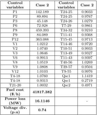
2) Case 2: OPF with Voltage Profile Improvement of IEEE57 Test System
Bus voltage enhancement is one of the most significant safety and service qualification indices. In order to as-sess this case, a two-fold objective function is consid-ered to minimize the operating fuel cost and enhancing the voltage profile at the same time by minimizing all the load bus deviations from the reference value. Volt-age profile, in this case, is compared to that of the precedent one as shown in Fig. 16 and the operating cost curve is shown in Fig. 17.
0,85 0,90 0,95 1,00 1,05 1,10 1,15 1 2 3 4 5 6 78 9 10 11 12 13 14 15 16 17 18 19 20 21 22 23 24 25 26 27 28 29 30 31 32 33 34 35 36 37 38 39 40 41 42 43 4445 4647 4849 5051 52535455
5657 bus voltagecase1
bus voltage case2
Fig. 16: Voltage improvement profile comparison.
It is clear that the voltage profile is enhanced effi-ciently compared with that in case 1. This could be achieved by the optimal tuning of the control param-eters within the constraints range as given in Tab. 16 using the proposed GWO technique.
It can be seen that the proposed GWO method con-verges to a better result than EADDE [7] method by decreasing the fuel cost from 42051.44 $/h to
Tab. 16: Performances measures for the TFC ($/h) in both cases.
System IEEE 30-bus system IEEE 57-bus system
Method GWO EADDE [6] MDE [35] PSO [14] GWO TSA [41] ABC [3] PSO [14]
Min 798.2934 800.204 802.376 800.409 41,684.00 41,685.07 41,781.00 41,688.68 Mean 798.6380 800.241 802.382 800.450 41,686.00 41,687.78 41,840.00 41,697.58 Max 800.1367 800.278 802.404 801.231 41,688.29 41,689.05 41,927.00 41,727.86 runs 40 30 40 20 50 50 20 20 50 100 150 200 Iteration 4.19 4.2 4.21 4.22 4.23 4.24 4.25
Best fuel cost ($/h)
104
GWO
Fig. 17: Convergence curve for IEEE57 in case 2.
41817.3826 $/h and voltage deviation from 0.7882 to 0.74.
Tab. 17: Optimal control variables settings for case 2.
Control variables Case 2 Control variables Case 2 P1 142.189 T24-25 0.9033 P2 89.894 T24-25 0.9767 P3 45.148 T24-26 1.0279 P6 72.928 T7-29 0.9861 P8 459.393 T34-32 0.9210 P9 84.089 T11-41 0.9368 P12 363.088 T15-45 0.9713 V1 1.0212 T14-46 0.9720 V2 1.0740 T10-51 0.9933 V3 1.0646 T13-49 0.9327 V6 0.9913 T11-43 0.9397 V8 1.0519 T40-56 1.0269 V9 1.0808 T39-57 0.9504 V12 1.0103 T9-55 0.9976 T4-18 1.0760 Qsc1 1.1419 T4-18 0.9313 Qsc1 0.2719 T21-20 1.0032 Qsc2 0.4971 Fuel cost ($/h) 41817.382 Power loss (MW) 16.1146 -Voltage div. (p.u) 0.74
From the comparison of the results shown in Tab. 16, it can be concluded that the solution quality of the GWO algorithm is very competitive and challenging because it converges to the best solution with less
com-putational time. Figure 18 presents the convergence curve for IEEE30 bus system after 40 runs and Fig. 19 the convergence curve for IEEE57-bus system after 50 runs. 5 10 15 20 25 30 35 40 Iteration 798.5 799 799.5 800 800.5 801
Best fuel cost ($/h)
GWO
Fig. 18: Convergence curves for IEEE57 with 50 runs.
5 10 15 20 25 30 35 40 45 50 Iteration 4.18 4.2 4.22 4.24 4.26 4.28
Best fuel cost ($/h)
104
GWO
Fig. 19: Convergence curves for IEEE57 with 50 runs.
5.
Conclusion
This paper presents an optimal power flow study us-ing a new meta-heuristic population-based search algo-rithm called Grey Wolf Optimizer (GWO). Considering
both wind and thermal power generators, in order to evaluate the effectiveness of the proposed technique; three case studies are considered in this work.
By adding to the normal operation condition, the N-1 contingency condition represented by lines outage and the uncertainty of wind power, which is modelled using Weibull distribution function is investigated.
Simulations results obtained by OPF analysis for two standard test systems IEEE-30, and IEEE-57 bus sys-tems without considering wind power are compared with results of other methods available in the litera-ture. The outcome of the comparison confirms the ef-fectiveness and robustness of the proposed algorithm.
Similarly, the results obtained in presence of wind en-ergy system were compared with those of other meth-ods reported in the literature using the IEEE 30 bus system. By increasing the value of reserve coefficient, the value of the injected amount in the system can be limited by the transmission system permissible ca-pacity of the existing network. On the other hand; when increasing the wind penetration level by increas-ing wind speed, the total operatincreas-ing cost decreases.
The method presents compromising performances measures compared to other methods found in the lit-erature. This analysis will be extended in the future to include spinning reserve in the main optimal power flow problem.
References
[1] ABOU, A. A., M. A. ABIDO and S. R. SPEA. Op-timal power flow using differential evolution algo-rithm.Electrical Engineering. 2009, vol. 91, iss. 2, pp. 69–78. ISSN 0948-7921. DOI: 10.1007/s00202-009-0116-z.
[2] CHANG, Y. C., T. Y. LEE, C. L. CHEN and R. M. JAN. Optimal power flow of a wind-thermal generation system. International Jour-nal of Electrical Power &Energy Systems. 2014, vol. 55, iss. 1, pp. 312–320. ISSN 0142-0615. DOI: 10.1016/j.ijepes.2013.09.028.
[3] REZAEI, M. and A. KARAMI. Artificial bee colony algorithm for solving multi-objective op-timal power flow problem. International Jour-nal of Electrical Power &Energy Systems. 2013, vol. 53, iss. 1, pp. 219–230. ISSN 0142-0615. DOI: 10.1016/j.ijepes.2013.04.021.
[4] BAKIRTZIS, A. G., P. N. BISKAS, C. E. ZOUMAS and V. PETRIDIS. Optimal power flow by enhanced genetic algorithm. IEEE Transac-tions on Power Systems. 2002, vol. 17, iss. 2,
pp. 229–236. ISSN 0885-8950. DOI: 10.1109/tp-wrs.2002.1007886.
[5] SURENDER, S. R., P. R. BIJWE and A. R. ABHYANKAR. Faster evolutionary algorithm base optimal power flow using incremental vari-ables.Electrical Power and Energy System. 2014, vol. 54, iss. 1, pp. 198–210. ISSN 0142-0615. DOI: 10.1016/j.ijepes.2013.07.019.
[6] VAISAKH, K. and L. R. SRINIVAS. Evolv-ing ant direction differential evolution for OPF with non-smooth cost functions. Engineer-ing Applications of Artificial Intelligence. 2011, vol. 24, iss. 3, pp. 426–436. ISSN 0952-1976. DOI: 10.1016/j.engappai.2010.10.019.
[7] ABACI, K. and V. YAMACLI. Differential search algorithm for solving multi-objective op-timal power flow problem. International Jour-nal of Electrical Power & Energy Systems. 2016, vol. 79, iss. 1, pp. 1–10. ISSN 0142-0615. DOI: 10.1016/j.ijepes.2015.12.021.
[8] GHASEMI, M., S. GHAVIDEL, M. GITI-ZADEH and E. AKBARI. An improved teaching–learning-based optimization algorithm using Levy mutation strategy for non-smooth optimal power flow. International Journal of Electrical Power & Energy Systems. 2015, vol. 65, iss. 1, pp. 375–384. ISSN 0142-0615. DOI: 10.1016/j.ijepes.2014.10.027.
[9] ROY, P. K. and C. PAUL. Optimal power flow using krill herd algorithm. International Transactions on Electrical Energy Systems. 2015, vol. 25, iss. 8, pp. 1397–1419. ISSN 2050-7038. DOI: 10.1002/etep.1888.
[10] ROA-SEPULVEDA, C. A. and B. J. PAVEZ-LAZO. A solution to the optimal power flow using simulated annealing. In: IEEE Porto Power Tech Proceedings. Porto: IEEE, 2001, pp. 5–9. ISBN 0-7803-7139-9. DOI: 10.1109/PTC.2001.964733. [11] BENTOUATI, B., S. CHETTIH, L. CHAIB
and V. SREERAM. Interior search algo-rithm for optimal power flow with non-smooth cost functions. Cogent Engineering. 2017, vol. 4, iss. 1, pp. 1–17. ISSN 2331-1916. DOI: 10.1080/23311916.2017.1292598.
[12] KUMARI, M. S. and S. MAHESWARAPU. Enhanced Genetic Algorithm based compu-tation technique for multi-objective Optimal Power Flow solution. International Journal of Electrical Power & Energy Systems. 2010, vol. 32, iss. 6, pp. 736–742. ISSN 0142-0615. DOI: 10.1016/j.ijepes.2010.01.010.
[13] BHATTACHARYA, A. and P. K. CHATTOPAD-HYAY. Application of biogeography-based optimi-sation to solve different optimal power flow prob-lems. IET Generation, Transmission & Distribu-tion. 2011, vol. 5, iss. 1, pp. 70–80. ISSN 1751-8687. DOI: 10.1049/iet-gtd.2010.0237.
[14] ABIDO, M. A. Optimal power flow using par-ticle swarm optimization. International Journal of Electrical Power & Energy Systems. 2002, vol. 24, iss. 7, pp. 563–571. ISSN 0142-0615. DOI: 10.1016/S0142-0615(01)00067-9.
[15] DUMAN, S., U. GUVENC, Y. SONMEZ and N. YORUKEREN. Optimal power flow using gravitational search algorithm. En-ergy Conversion and Management. 2012, vol. 59, iss. 1, pp. 86–95. ISSN 0196-8904. DOI: 10.1016/j.enconman.2012.02.024.
[16] VAISAKH, K., L. R. SRINIVAS and K. MEAH. Genetic evolving ant direction PSODV hy-brid algorithm for OPF with non-smooth cost functions. Electrical Engineering. 2013, vol. 95, iss. 3, pp. 185–199. ISSN 0948-7921. DOI: 10.1007/s00202-012-0251-9.
[17] KUMAR, R. A. and L. PREMALATHA. Op-timal power flow for a deregulated power sys-tem using adaptive real coded biogeography-based optimization. International Journal of Electrical Power & Energy Systems. 2015, vol. 73, iss. 1, pp. 393–399. ISSN 0142-0615. DOI: 10.1016/j.ijepes.2015.05.011.
[18] KHAMEES, K. A., A. E. RAFEI, N. M. BADRA and A. Y. ABDELAZIZ. Solution of optimal power flow using evolutionary-based algorithms.
International Journal of Engineering, Science and Technology. 2017, vol. 9, no. 1, pp. 55–68. ISSN 2141-2839.
[19] ROY, R. and H. T. JADHAV. Optimal power flow solution of power system incorporating stochastic wind power using Gbest guided arti-ficial bee colony algorithm. International Jour-nal of Electrical Power &Energy Systems. 2015, vol. 64, no. 1, pp. 562–578. ISSN 0142-0615. DOI: 10.1016/j.ijepes.2014.07.010.
[20] MASKAR, M. B., A. R. THORAT, P. D. BA-MANE and I. KORACHGAON. Optimal power flow incorporating thermal and wind power plant. In: International Conference on Cir-cuit, Power and Computing Technologies. Kollam: IEEE, 2017, pp. 1–6. ISBN 978-1-5090-4967-7. DOI: 10.1109/ICCPCT.2017.8074265.
[21] JIANG, S., Z. JI and Y. WANG. A novel grav-itational acceleration enhanced particle swarm
optimization algorithm for wind–thermal eco-nomic emission dispatch problem considering wind power availability. International Journal of Electrical Power & Energy Systems. 2015, vol. 73, iss. 1, pp. 1035–1050. ISSN 0142-0615. DOI: 10.1016/j.ijepes.2015.06.014.
[22] PANDA, A. and M. TRIPATHY. Security constrained optimal power flow solution of wind-thermal generation system using modi-fied bacteria foraging algorithm. Energy. 2015, vol. 93, iss. 1, pp. 816–827. ISSN 0360-5442. DOI: 10.1016/j.energy.2015.09.083.
[23] MISHRA, S., Y. MISHRA and S. VIGNESH. Security constrained economic dispatch consider-ing wind energy conversion systems. In: IEEE Power and Energy Society General Meeting. De-troit: IEEE, 2011, pp. 1–8. ISBN 978-1-4577-1000-1. DOI: 10.1109/PES.201978-1-4577-1000-1.6039544.
[24] SULAIMAN, M. H., Z. MUSTAFFA, M. R. MO-HAMED and O. ALIMAN. Using the gray wolf optimizer for solving optimal reactive power dis-patch problem. Applied Soft Computing. 2015, vol. 32, iss. 1, pp. 286–292. ISSN 1568-4946. DOI: 10.1016/j.asoc.2015.03.041.
[25] EL-FERGANY, A. A. and H. M. HASANIEN. Single and Multi-objective Optimal Power Flow Using Grey Wolf Optimizer and Differ-ential Evolution Algorithms. Electric Power Components and Systems. 2015, vol. 43, iss. 13, pp. 1548–1559. ISSN 1532-5008. DOI: 10.1080/15325008.2015.1041625.
[26] IAHKALI, H. and M. VAKILIAN. Stochastic unit commitment of wind farms integrated in power system. Electric Power Systems Research. 2010, vol. 80, iss. 9, pp. 1006–1017. ISSN 0378-7796. DOI: 10.1016/j.epsr.2010.01.003.
[27] MIRJALILI, S., S. M. MIRJALILI and A. LEWIS. Grey Wolf Optimizer. Ad-vances in Engineering Software. 2014, vol. 69, iss. 9, pp. 46–61. ISSN 0965-9978. DOI: 10.1016/j.advengsoft.2013.12.007.
[28] MIRJALILI, S. and S. Z. M. HASHIM. A new hybrid PSOGSA algorithm for function optimiza-tion. In: International Conference on Computer and Information Application. Tianjin: IEEE, 2010, pp. 374–377. ISBN 978-1-4244-8598-7. DOI: 10.1109/ICCIA.2010.6141614.
[29] BAI, W., D. LEE and K. LEE. Stochas-tic Dynamic Optimal Power Flow Integrated with Wind Energy Using Generalized Dy-namic Factor Model.IFAC-Papers OnLine. 2016, vol. 49, iss. 27, pp. 129–134. ISSN 2405-8963. DOI: 10.1016/j.ifacol.2016.10.731.
[30] XIE, L., H. D. CHIANG and S. H. LI. Op-timal power flow calculation of power sys-tem with wind farms. In: IEEE Power and Energy Society General Meeting. Detroit: IEEE, 2011, pp. 1–6. ISBN 978-1-4577-1000-1. DOI: 10.1109/PES.2011.6039105.
[31] MONDAL, S., A. BHATTACHARYA and S. H. NEE-DEY. Multi-objective economic emission load dispatch solution using gravita-tional search algorithm and considering wind power penetration. International Journal of Electrical Power & Energy Systems. 2013, vol. 44, iss. 1, pp. 282–292. ISSN 0142-0615. DOI: 10.1016/j.ijepes.2012.06.049.
[32] MOHAMED, A. A., A. M. EL-GAAFARY, Y. S. MOHAMED and A. M. HEMEIDA. Multi-objective Modified Grey Wolf Optimizer for Optimal Power Flow. In: Eighteenth Interna-tional Middle East Power Systems Conference (MEPCON). Cairo: IEEE, 2016, pp. 982–990. ISBN 978-1-4673-9063-7. DOI: 10.1109/MEP-CON.2016.7837016.
[33] KAPOOR, S., I. ZEYA, C. SINGHAL and S. J. NANDA. A Grey Wolf Optimizer Based Auto-matic Clustering Algorithm for Satellite Image Segmentation. Procedia Computer Science. 2017, vol. 115, iss. 1, pp. 415–422. ISSN 1877-0509. DOI: 10.1016/j.procs.2017.09.100.
[34] ANANTASATE, S. and P. BHASAPUTRA. A objective bees algorithm for multi-objective optimal power flow problem. In: The 8th Electrical Engineering/ Electronics, Computer, Telecommunications and Information Technology (ECTI) Association of Thailand. Khon Kaen: IEEE, 2011, pp. 852–856. ISBN 978-1-4577-0425-3. DOI: 10.1109/ECTICON.2011.5947974. [35] SAYAH, S. and K. ZEHAR. Modified
dif-ferential evolution algorithm for optimal power flow with non-smooth cost functions.
Energy Conversion and Management. 2008, vol. 49, iss. 11, pp. 3036–3042. ISSN 0196-8904. DOI: 10.1016/j.enconman.2008.06.014.
[36] BOUCHEKARA, H. R. E. H. Optimal power flow using black-hole-based optimization approach. Applied Soft Computing. 2014, vol. 24, iss. 1, pp. 879–888. ISSN 1568-4946. DOI: 10.1016/j.asoc.2014.08.056.
[37] ZIMMERMAN, R., C. MURILLO-SANCHEZ and D. GAN. Matlab power System Simulation Package. New York: School of Electrical Engineer-ing, Cornell University, 2007.
[38] SINSUPAN, N., U. LEETON and T. KUL-WORAWANICHPONG. Application of har-mony search to optimal power flow prob-lems. In: International Conference on Ad-vances in Energy Engineering. Beijing: IEEE, 2010, pp. 219–222. ISBN 978-1-4244-7831-6. DOI: 10.1109/ICAEE.2010.5557575.
[39] REDDY, S. S., and C. SRINIVASA RATH-NAM. Optimal Power Flow using Glowworm Swarm Optimization. International Journal of Electrical Power & Energy Systems. 2016, vol. 80, iss. 1, pp. 128–139. ISSN 0142-0615. DOI: 10.1016/j.ijepes.2016.01.036.
[40] REGALADO, J. A., B. E. EMILIO and E. CUEVAS. Optimal power flow solution using Modified Flower Pollination Algorithm. In: IEEE International Autumn Meeting on Power, Electronics and Computing. Ixtapa: IEEE, 2015, pp. 1–6. ISBN 978-1-4673-7121-6. DOI: 10.1109/ROPEC.2015.7395073.
[41] EL-FERGANY, A. A. and H. M. HASANIEN. Tree-seed algorithm for solving optimal power flow problem in large-scale power systems incorpo-rating validations and comparisons. Applied Soft Computing. 2018, vol. 64, iss. 1, pp. 307–316. ISSN 1568-4946. DOI: 10.1016/j.asoc.2017.12.026.
About Authors
Sebaa HADDI was born in Setif, Algeria. He received his M.Sc. from University of Setif in 1997. follows his study in the University of Ferhat Abbes Setif 1, has got his B.Sc. degree in Electrical Engi-neering Power system from Setif University (Algeria) in 1997, and his M.Sc. degree in 2009 in the field of electrical network, now he prepares for the Doctorate degree in the Department of Electrical Engineering, of the university of Setif, His research interests include the optimization in power system, optimal integration of renewable sources, Facts device.
Omrane BOUKETIR was born in Setif, Algeria. He received his M Eng. in Electrical Automation from Setif University (Algeria) in 1995. In 1999 he obtained his M.Sc. degree from University Putra Malaysia in the field of Automation and Robotics and Ph.D. degree in power electronics systems from the same university in 2005. His research areas include power electronics and drive systems, SiC switching devices, CAD tools in electrical engineering and trends and methods in tertiary education.
Tarek BOUTKIR was born in Setif, Algeria. He received his M.Sc. in Electrical Engineering Power system from Setif University (Algeria) in 1994, his
M.Sc. degree from Annaba University in 1998, his Ph.D. degree in power system from Batna University (Algeria) in 2003. His areas of interest are the application of the meta-heuristic methods in opti-mal power flow, FACTS control and improvement in
electric power systems, Multi-Objective Optimization for power systems, and Voltage Stability and Security Analysis. He is the Editor-In-Chief of Journal of Electrical Systems (Algeria), the Co-Editor of Journal of Automation & Systems Engineering (Algeria).