for Time Series Forecasting
Paulo Cortez1, and Juan Peralta Donate21 Centro Algoritmi, Departamento de Sistemas de Informa¸c˜ao, Universidade do Minho, 4800-058 Guimar˜aes, Portugal
[email protected] http://www3.dsi.uminho.pt/pcortez
2 Computer Science Department, University Carlos III of Madrid, Av. de la Universidad 30 28911 Leganes, Spain
Abstract. Time Series Forecasting (TSF) uses past patterns of an event in order to predict its future values and is a key tool to support decision making. In the last decades, Computational Intelligence (CI) techniques, such as Artificial Neural Networks (ANN) and more recently Support Vector Machines (SVM), have been proposed for TSF. The accuracy of the best CI model is affected by both the selection of input time lags and the model’s hyperparameters. In this work, we propose a novel Evolutionary SVM (ESVM) approach for TSF based on the Estimation Distribution Algorithm to search for the best number of inputs and SVM hyperparameters. Several experiments were held, using a set of six time series from distinct real-world domains. Overall, the proposed ESVM is competitive when compared with an Evolutionary ANN (EANN) and the popular ARIMA methodology, while consuming less computational effort when compared with EANN.
Keywords: Evolutionary Computation, Support Vector Machines, Time Series, Forecasting.
1
Introduction
Forecasting the future using past data is an important tool to reduce uncertainty and support both individual and organization decision making. In particular, multi-step ahead predictions (e.g., issued several months in advance) are useful to aid tactical decisions, such as planning production resources or evaluating alternative economic strategies [2]. The field of Time Series Forecasting (TSF) deals with the prediction of a given phenomenon (e.g., umbrella sales) based on the past patterns of the same event. TSF has become increasingly used in distinct areas such as Agriculture, Finance, Production or Sales [14].
The research reported here has been supported by FEDER (program COMPETE and FCT) under project FCOMP-01-0124-FEDER-022674.
A.E.P. Villa et al. (Eds.): ICANN 2012, Part II, LNCS 7553, pp. 523–530, 2012. c
Several Operational Research TSF methods have been proposed, such as Holt-Winters (in the sixties) or the ARIMA methodology [14] (in the seventies). More recently, several Computational Intelligence (CI) methods have been applied to TSF, such as Artificial Neural Networks (ANN) [12,6], and Support Vector Ma-chines (SVM) [15,9,3]. CI models such as ANNs and SVMs are natural solutions for TSF, since they are more flexible (i.e., no a priori restriction is imposed) when compared with classical TSF models, presenting nonlinear learning capa-bilities. When compared with ANN, SVM presents theoretical advantages, such as the absence of local minima in the learning phase.
When applying these CI methods to TSF, variable and model selection are critical issues. A sliding time window is often used to create a set of training examples from the series. A small time window will provide insufficient infor-mation, while using a large number of time lags will increase the probability of having irrelevant inputs. Thus, variable selection is useful to discard irrelevant time lags, leading to simpler models that are easier to interpret and that usually give better performances [4,9,6]. On the other hand, CI models such as ANN and SVM have hyperparameters that need to be adjusted (e.g., number of ANN hidden nodes or kernel parameter) [8]. Complex models may overfit the data, losing the capability to generalize, while a model that is too simple will present limited learning capabilities.
Several hybrid systems, which combine two or more CI techniques, have also been proposed for TSF, such as Evolutionary ANN (EANN) [4]. Most EANNs use the standard Genetic Algorithm (GA). More recently, the Estimation Dis-tribution Algorithm (EDA) was proposed [13]. Such algorithm uses exploitation and exploration properties to find a good solution. In [16], EDA was used as the search engine of an EANN, outperforming a GA based EANN. Following this result, in this paper we propose a novel Evolutionary SVM (ESVM) ap-proach based on the EDA engine, in order to automatically select the best SVM multi-step ahead forecasting model. Moreover, we also compare ESVM with the EANN proposed in [16] and the popular ARIMA methodology.
The paper is organized as follows. First, Section 2 describes the ESVM ap-proach. Next, Section 3 presents the experimental setup and the obtained results. Finally, the paper is concluded in Section 4.
2
Evolutionary Support Vector Machine
2.1 Time Series Forecasting
The problem of TSF using CI models, such as ANN [16] or SVM [3], is considered as obtaining the relationship from the value at periodyt and the values from
previous elements of the time series, using several time lags{t−1, t−2, . . . , t−I}, to obtain a function as it is shown in [16]:
ˆ
yt=f(yt−1, yt−2, . . . , yt−I) (1) where ˆytdenotes the estimated forecast as given by the functionf (e.g., SVM), andI the number of input values.
In order to obtain a single model to forecast time series values, an initial step has to be done with the original values of the time series, i.e., normalizing the data. The original values (yt) are normalized into the range [0,1] (leading to the Nt values). Once the model outputs the resulting values, the inverse process is carried out, rescaling them back to the original scale. Only one output was chosen and multi-step ahead forecasts are built by iteratively using 1-ahead predictions as inputs [4]. Therefore, the time series is transformed into a patterns set depending on theI inputs of a particular model, each pattern consisting of:
– Iinputs values: with theI-th normalized previous valuesNt−1, Nt−2, ..., Nt−I.
– one output value:Nt(the desired target).
This patterns set will be used to train and validate each model generated dur-ing the evolutionary execution. Thus, the patterns set is split into two subsets, training (with the first 70% elements of the series) and validation (with the remaining ones), under a timely ordered holdout scheme.
2.2 Evolutionary Support Vector Machine Design
The problem of designing SVM for TSF can be seen as a search problem into the space of all possible solutions. While several Evolutionary Computation methods could be used for this search, we adopt the EDA algorithm, since it has outper-formed the standard GA in our previous work [16]. When designing a ESVM, there are three crucial issues: i) setting the solution’s space, i.e., what informa-tion of the SVM is previously set and what is included into the chromosome; ii) how each solution is codified into a chromosome, i.e., encoding schema; and iii) what are we optimizing, i.e., defining the fitness function.
When designing a SVM, there are three crucial issues it should be taken into account: the type of SVM to use, the selection of the kernel function and tuning the parameters associated with the two previous selections. Since TSF is a particular regression case, for the SVM type and kernel, we selected the popular
ε-insensitive loss function (known asε-SVR) and Gaussian kernel combination, as implemented in the LIBSVM tool [1]. In SVM regression [17], the inputy= (yt−kI, . . . , yt−k2, yt−k1), for a SVM with I inputs, is transformed into a high m-dimensional feature space, by using a nonlinear mapping (φ) that does not need to be explicitly known but that depends of a kernel function. Then, the SVM algorithm finds the best linear separating hyperplane, tolerating a small error (ε) when fitting the data, in the feature space:
ˆ yt=w0+ m j=1 wjφj(y) (2)
This model requires setting three parameters:γ– the Gaussian kernel parameter,
exp(−γ||x−x||2), γ > 0; C – a trade-off between fitting the errors and the flatness of the mapping; andε- the width of theε-insensitive tube.
In this paper, an evolving hybrid system that uses EDA and SVM, is adopted. Following the suggestion of the LIBSVM authors [1], SVM parameters are
searched in terms an exponentially growing scale. We also take into account the number of input values of the time series (I) used to train the SVM. There-fore, we adopt a direct encoding scheme, using a numeric representation with 8 genes, according to the chromosomeg1g2g3g4g5g6g7g8, such that:
I= round(α·n·10g1+g2+1 100 ), g1∈ {0,1, ...,9} ∧g1∈ {0,1, ...,9} γ= 2(g3+g104)−5 , g 3∈ {−9,−8, ...,9} ∧g4∈ {−9,−8, ...,9} C= 2(g5+g106)+5 , g 5∈ {−9,−8, ...,9} ∧g6∈ {−9,−8, ...,9} ε= 2(g7+g108)−8 , g 7∈ {−9,−8, ...,9} ∧g8∈ {−9,−8, ...,9} (3)
wheregi denotes the i-th gene of the chromosome. The input search range
in-cludes only integer numbers, due to the use of round function, and depends onn, the length of the time series (#in-samples or training data), scaled by a constant α factor. Based on our previous research using EANN for TSF [16], we set α = 0.45. Thus, the ranges for the search space are: I, depends on the series length (e.g., I∈ {3,7,10,13,17, ...,331}for Quebec); γ∈2[−14.9,4.9];
C∈2[−4.9,14.9]; and ε∈2[−17.9,1.9].
The evolutionary process consists of the following steps:
1. First, a randomly generated population (composed of to 50 individuals), i.e., a set of randomly generated chromosomes, is obtained.
2. The phenotypes (SVM model) and fitness value of each individual of the actual generation is obtained. This includes the steps:
(a) The phenotype of an individual of the actual generation is first obtained (using LIBSVM [1]).
(b) Then, for each model, training and validation subsets are obtained from time series data depending on the number of inputs nodes, as it was explained in Section 2.1.
(c) The model is fitted using the Sequential Minimal Optimization algo-rithm, as implemented in LIBSVM. The fitness for each individual is given by the Mean Squared Error (MSE) validation error, during the learning process. The aim is to reduce extreme errors (e.g., outliers) that can highly affect multi-step ahead forecasts. Moreover, preliminary experiments (with time series not present in Table 1), have shown that this choice leads to better forecasts when compared with absolute errors. 3. Once the fitness values for whole population have been already obtained, UMDA-EDA (with no dependencies between variables) [16] operators (se-lection, estimation of the empirical probability distribution and sampling solutions) are applied in order to generate the population of the next gener-ation, i.e., a new set of chromosomes.
4. Steps 2 and 3 are iteratively executed until a maximum number of genera-tions is reached.
The parameters of the EDA (e.g., population size of 50) were set to the same values used by the EANN proposed in [16]. Since the EDA works as a second order optimization procedure, the tuning of its internal parameters is not a critical issue (e.g., using a population of 48 does not does not substantially change the results). Also, this EDA has a fast convergence (shown in Fig. 1).
3
Experiments and Results
3.1 Time Series
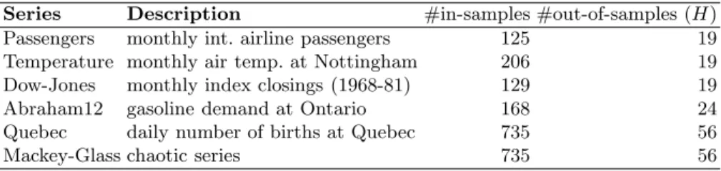
We selected a total of six time series, with different characteristics and from distinct domains (Table 1). Five series were selected from the well-known Hyn-dman’s time series data library repository [10]. These are named Passengers, Temperature, Dow-Jones, Quebec and Abraham12. We also adopt the Mackey-Glass series, which is a common nonlinear benchmark. It should be noted that these six times series were also adopted by theNN3 andNN5 forecasting com-petitions [5]. Except for Mackey-Glass, all datasets are from real-world domains and such data can be affected by external issues (e.g., strikes), which make them interesting datasets and more difficult to predict.
Table 1.Time series data
Series Description #in-samples #out-of-samples (H) Passengers monthly int. airline passengers 125 19 Temperature monthly air temp. at Nottingham 206 19 Dow-Jones monthly index closings (1968-81) 129 19
Abraham12 gasoline demand at Ontario 168 24
Quebec daily number of births at Quebec 735 56
Mackey-Glass chaotic series 735 56
3.2 Evaluation
The Symmetric Mean Absolute Percentage Error (SMAPE) is given by [11]:
SMAP E= 1 H T+H t=T+1 |et| (|yt|+|yˆt|)/2 ×100% (4)
whereet=yt−ytˆ,Tis the current time period andH is the forecasting horizon, the number of multi-step ahead forecasts. SMAPE is a popular forecasting metric that has the advantage of being scale independent when compared with MSE, thus can be more easily used to compare methods across different series, ranging from 0% to 200%. SMAPE was also the error metric used in NN3, NN5 and
NNGC1 forecasting competitions [5].
3.3 Results
For the comparison, we have chosen the EANN presented in [16], which is similar to ESVM except that is uses a multilayer perceptron trained with the RPROP algorithm, as implemented using the SNNS tool [18]. EANN optimizes the num-ber of inputs (I∈ {1, ...,100}) and hidden nodes (from 0 to 99) and the RPROP parameters (Δ0∈ {1,0.01,0.001, . . .,10−9}andΔmax∈ {0,1, ...,99}). Both the
Table 2.Forecasting errors (%SMAPE, best values inbold) and best SVM models Time SeriesARIMA EANN ESVM I γ C ε
Passengers 4.50 3.39 5.35 14 2−4.1 212.7 2−8.6 Temperature 3.42 3.51 4.42 79 2−1.9 2−0.5 2−8.8 Dow-Jones 4.78 6.28 6.35 19 2−13.3 210.5 2−5.3 Abraham12 6.20 4.71 4.86 28 2−13.1 214.9 2−15.0 Quebec 10.36 10.83 9.31 301 2−13.6 212.7 2−16.3 Mackey-glass 26.20 7.06 1.32 10 22.0 21.70 2−16.0 Average 9.24 5.96 5.27 Median 5.49 5.49 5.11
ESVM and EANN experiments were conducted using code written in the C lan-guage by the authors. As the stopping criterion, we used a maximum of 100 generations for ESVM and EANN. For a baseline comparison, we have also cho-sen the ARIMA methodology, as computed by the ForecastPro ctool [7]. The rationale is to use a popular benchmark that can easily be compared and that does not require expert model selection capabilities from the user. The obtained results are shown in Table 2 (SMAPE errors and best SVM models).
0 20 40 60 80 100 0.00 0.02 0.04 0.06 0.08 generations fitness (MSE o v er nor maliz ed data) 0 5 10 15 0.000 0.005 0.010 0.015 PassengersTemperature Dow−Jones Abraham12 Quebec Mackey−Glass ● ● ● ● ● ● ● ● ● ● ● ● ● ● ● ● ● ● ● ● ● ● ● ● ●● ● ● ● ● ● ● ● ● ● ● ● ● ● ● ● ● ● ● ● ● ● ● ● ● ● ● ● ● ● ● 0 10 20 30 40 50 200 250 300 Quebec (SMAPE=9.31)
Horizon (ahead forecasts)
V
alues
● ESVM Quebec
Fig. 1.Evolution of the ESVM best fitness value for all series (left, includes a zoom of the bottom left area) and example of the ESVM forecasts for Quebec (right)
An analysis to tables shows that the proposed ESVM provides interesting forecasts when compared with EANN and ARIMA. Each forecasting approach is the best option for two series. Yet, ESVM provides the lowest average and median (over all series, last two rows) results. The left of Fig. 1 plots the evolution of
Table 3.Comparison of computational effort required by ESVM and EANN
Time EANN ESVM Rt
Series time (min) time (min) Passengers 165 5 96.7% Temperature 315 6 98.1% Dow-Jones 161 3 98.2% Abraham12 420 6 98.6% Quebec 6603 95 98.5% Mackey-glass 5649 105 98.1%
the best fitness values for ESVM (left), showing a fast convergence of the EDA algorithm for all series. For demonstration purposes, the right of Fig. 1 plots the ESVM forecasts for Quebec, showing a good fit.
The experimentation was carried out with an exclusive access to a server (Intel Xeon 2.27 GHz processor using Linux). Table 3 shows the computational time (in minutes) required by each evolutionary method and series. The last column shows in percentage, the reduction of computational effort obtained by ESVM when compared with EANN, where Rt = 1−(tESVM/tEANN) and tM is the time required for modelM. As shown by the table, ESVM consumes much less computational effort in all the time series tested. It can be observed a reduction rate of at least 96% in all cases.
4
Conclusions
This paper proposes a novel Evolutionary Support Vector Machine (ESVM) method for multi-step ahead TSF, which automatically searches best number of inputs and SVM hyperparameters. The proposed ESVM was compared against two approaches, an Evolutionary Artificial Neural Network (EANN) and the popular ARIMA methodology. The experiments held using six time series from distinct domains, revealed the proposed ESVM as the best forecasting method. Moreover, when compared with EANN, ESVM requires much less computational effort, with a reduction rate (in terms of time elapsed) greater than 96%. Thus, ESVM is a good tool to quickly obtain accurate forecasts and this is a useful characteristic for several TSF domains, such as critical or control systems. In the future, we intend to address other SVM kernels (e.g., Polynomial) and extend the experimentation to include time series from more domains (e.g., Medical data).
References
1. Chang, C.-C., Lin, C.-J.: LIBSVM: A library for support vector machines. ACM Transactions on Intelligent Systems and Technology 2, 27:1–27:27 (2011)
3. Cortez, P.: Sensitivity Analysis for Time Lag Selection to Forecast Seasonal Time Series using Neural Networks and Support Vector Machines. In: Proceedings of the International Joint Conference on Neural Networks (IJCNN 2010), pp. 3694–3701. IEEE, Barcelona (2010)
4. Cortez, P., Rocha, M., Neves, J.: Time Series Forecasting by Evolutionary Neural Networks. In: Artificial Neural Networks in Real-Life Applications, ch. III, pp. 47–70. Idea Group Publishing, USA (2006)
5. Crone, S.: Time series forecasting competition for neural networks and compu-tational intelligence (2011),http://www-.neural--forecastingcompetition.com
(accessed on January 2011)
6. Crone, S.F., Kourentzes, N.: Feature selection for time series prediction - a com-bined filter and wrapper approach for neural networks. Neurocomputing 73, 1923– 1936 (2010)
7. Goodrich, R.L.: The Forecast Pro methodology. International Journal of Forecast-ing 16(4), 533–535 (2000)
8. Hastie, T., Tibshirani, R., Friedman, J.: The Elements of Statistical Learning: Data Mining, Inference, and Prediction. Springer, NY (2008)
9. He, W., Wang, Z., Jiang, H.: Model optimizing and feature selecting for sup-port vector regression in time series forecasting. Neurocomputing 72(1-3), 600–611 (2008)
10. Hyndman, R.: Time Series Data Library (2011),http://robjhyndman.com/TSDL/
(accessed on January 2011)
11. Hyndman, R.J., Koehler, A.B.: Another look at measures of forecast accuracy. International Journal of Forecasting 22(4), 679–688 (2006)
12. Lapedes, A., Farber, R.: Non-Linear Signal Processing Using Neural Networks: Prediction and System Modelling. Technical Report LA-UR-87-2662, Los Alamos National Laboratory, USA (1987)
13. Larranaga, P., Lozano, J.A.: Estimation of distribution algorithms: A new tool for evolutionary computation, vol. 2. Springer (2002)
14. Makridakis, S., Wheelwright, S.C., Hyndman, R.J.: Forecasting methods and ap-plications, 3rd edn. John Wiley & Sons, USA (2008)
15. Miiller, K., Smola, A., Ratsch, G., Scholkopf, B., Kohlmorgen, J., Vapnik, V.: Predicting Time Series with Support Vector Machines. In: Gerstner, W., Hasler, M., Germond, A., Nicoud, J.-D. (eds.) ICANN 1997. LNCS, vol. 1327, pp. 999– 1004. Springer, Heidelberg (1997)
16. Peralta, J., Gutierrez, G., Sanchis, A.: Time series forecasting by evolving artificial neural networks using genetic algorithms and estimation of distribution algorithms. In: The 2010 International Joint Conference on Neural Networks (IJCNN), pp. 1–8 (July 2010)
17. Smola, A., Sch¨olkopf, B.: A tutorial on support vector regression. Statistics and Computing 14, 199–222 (2004)
18. Zell, A., Mache, N., Huebner, R., Mamier, G., Vogt, M., Schmalzl, M., Herrmann, K.U.: Snns (stuttgart neural network simulator). In: Neural Network Simulation Environments, pp. 165–186 (1994)