DYNAMIC EVOLUTIONARY OPTIMIZATION WITH
PARTICLE SWARM OPTIMIZATION
By
SURYAKIRAN CHAVALI K V RAMANA
Bachelor of Technology in Instrumentation and Control
National Institute of Technology
Tiruchchirappalli, Tamil Nadu, India
2012
Submitted to the Faculty of the
Graduate College of the
Oklahoma State University
in partial fulfillment of
the requirements for
the Degree of
MASTER OF SCIENCE
ii
DYNAMIC EVOLUTIONARY OPTIMIZATION WITH
PARTICLE SWARM OPTIMIZATION
Thesis Approved:
Dr. Gary Yen Thesis Adviser Dr. Carl Latino
iii
Acknowledgements reflect the views of the author and are not endorsed by committee members or Oklahoma State University.
ACKNOWLEDGEMENTS
I would like to express my sincere gratitude to my thesis advisor and academic mentor, Dr. Gary G. Yen for his continuous support and motivation during my master’s study and research. The knowledge he shared with me, the kind of trust he had instilled in me, the degree of patience he embraced when correcting my mistakes, are some things that made me admire him a lot. I am extremely fortunate to have an advisor like him. Without Dr. Yen, this research work would not have been completed or written.
I would also like to express my gratitude to Dr. Subhash Kak and Dr. Carl Latino for being members of my Graduate Committee and I would also like to thank them for attending my defense amidst their busy schedule. I would also like to extend my sincere thanks to the school of Electrical and Computer Engineering at Oklahoma State University for giving me the opportunity to pursue my graduate education.
I am extremely thankful to my roommates and friends Nakul Babu Maddipati, Suresh Babu Myneni, Gopal Koya and Sri Theja Vuppala for their encouragement and support during my graduate study.
I would like to acknowledge, with deepest gratitude, the support and immeasurable love of my family. My parents, Satyanarayana Murti Chavali and Padmavathi Chavali, have supported me at each and every phase of my career. They gave me freedom to take my own decisions and gave up many things for me to chase my dreams. I can never be grateful enough to such an amazing parents. Nothing is happier to me than making them feel proud for my achievements.
iv
Name: SURYAKIRAN CHAVALI K V RAMANA
Date of Degree: DECEMBER, 2015
Title of Study: DYNAMIC EVOLUTIONARY OPTIMIZATION WITH PARTICLE
SWARM OPTIMIZATION
Major Field: ELECTRICAL ENGINEERING
Abstract: Many real world optimization problems have to be solved in the presence of uncertainties. An optimization algorithm has to perform satisfactorily under the presence of such dynamic changes in the environment. In addition to it, the algorithm also has to justify for the additional computational cost incurred. Multi population approaches are found very effective in tracking and locating dynamic optima. In addition, it is necessary to reuse the information from the past evolutions as it facilitates a faster and effective convergence after the occurrence of the change. This thesis proposes a new dynamic particle swarm optimization technique that uses multiple swarms to locate a set of optimal solutions and effectively exploits the past information and adapts the population to the corresponding new locations using the concept of relocation radius. The proposed algorithm uses an adaptive hierarchical clustering mechanism to form multiple swarms. The relocation radius is determined based on the change in the functional values of the particles due to change in the environment and the average sensitivities of the decision variables to the corresponding change in the objective space. The newly adapted population is fitter compared to the original population or a randomly initialized population. The algorithm is tested on dynamic benchmark functions and compared to some of the state-of-the-art dynamic evolutionary algorithms and the results are found to be promising. The algorithm performs better than most of the existing algorithms proposed in literature.
v
TABLE OF CONTENTS
Chapter
Page
I. INTRODUCTION ...1
1.1 Overview ...1
1.2 Problem Definition...2
1.2.1 Dynamic optimization problem ...2
1.3 Particle Swarm Optimization ...3
1.4 Research Goal and Approach...5
1.5 Document Organization ...6
II. DYNAMIC EVOLUTIONARY OPTIMIZATION ...7
2.1 Introduction ...7
2.2 Types of Fitness Landscapes ...10
2.3 Characteristics of Dynamic Optimization Problems...11
2.3.1 Severity of Change ...12
2.3.2 Frequency of Change ...12
2.3.3 Observability and Detectability ...12
2.3.4 Dynamic of Change ...13
2.4 Literature Review...13
2.4.1 Introducing Diversity ...13
2.4.2 Maintaining Diversity ...15
2.4.3 Memory Approaches ...16
2.4.4 Multi-population Approaches ...18
2.4.5 Self-Adaptation and Mutation...19
2.5 Performance Metrics ...20
2.5.1 Offline Error Variation ...20
2.5.2 Adaptation Performance ...21
2.6 Benchmark Problems for Dynamic Optimization Algorithms ...21
2.7 Summary ...24
III. PROPOSED DYNAMIC PARTICLE SWARM OPTIMIZATION ...25
3.1 Creating Multiple Sub-swarms ...25
3.2 Local Search Strategy ...29
vi
Chapter
Page
3.4 Change Detection ...33
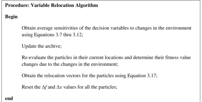
3.5 Introducing Diversity using Variable Relocation Algorithm...33
3.6 Summary ...38
IV. EXPERIMENTAL SIMULATION RESULTS AND DISCUSSION ...41
4.1 Experimental Setup ...41
4.2 Experimental Investigation of the Algorithm ...42
4.3 Comparison with peer algorithms ...48
4.4 Summary ...50
V. CONCLUSION AND FUTURE RECOMMENDATIONS ...51
vii
LIST OF TABLES
Table
Page
4.1 Default Experimental parameter settings for MPB problem ...42
4.2 Offline Error Variation of Different parameter configurations ...44
4.3 Number of sub-swarms created by Clustering Method ...45
4.4 Number of peaks found by algorithm on MPB problem ...45
4.5 Offline Error Variation of Algorithms on MPB problem as a function of number
of peaks ...48
4.6 Adaptation Performance of Algorithms on MPB problem as a function of
number of peaks ...49
4.7 Offline Error Variation on MPB problem with 10 peaks as a function of
Generations between Changes ...50
viii
LIST OF FIGURES
Figure
Page
1.1 Pseudo-code for a typical Particle Swarm Optimization algorithm ...4
2.1 Dynamic Changes occurring in the Fitness Landscape ...7
2.2 Dynamic Fitness Landscape ...11
3.1 Pseudo-code for performing Clustering algorithm to form Sub-swarms ...27
3.2 Pseudo-code for the FindNearestPair Algorithm ...28
3.3 Pseudo-code for performing local search on a sub-swarm S ...30
3.4 Pseudo-code for performing Redundancy Control ...32
3.5 Variable Relocation algorithm for re-initializing the particles ...38
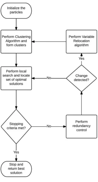
3.6 Flow chart for the proposed Dynamic Particle Swarm Optimization ...40
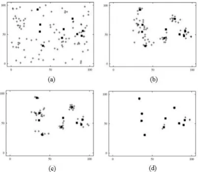
4.1 Particle Locations at different evaluations ...43
4.2 Offline Error Variation with Different Configurations on MPB problem with
different number of peaks ...46
4.3 Offline Error of varying β with different number of peaks ...47
4.4 Offline Error Variation of Algorithms on MPB problem as a function of number
of peaks ...49
1
CHAPTER I
INTRODUCTION
1.1 Overview
Optimization is considered among the most important problems in mathematics and sciences. The importance of optimization and its numerous applications have inspired scientists to investigate on different aspects of the problem. There are many real-world applications that involve optimization and the goal in all these problems is to either maximize or minimize one or more cost functions considering several limitations such as changing conditions, involvement of constraints, noise etc [1]. While there are limitations in a problem space it could be solved easily, however, increasing limitations leads to a much harder problem which requires a more sophisticated complex mechanism. This thesis focuses on problems that are subject to dynamic conditions.
Many real world optimization problems are subject to changing conditions over time. These types of problems are termed as the dynamic optimization problems. The changes in the conditions include changes in the objective function, the problem instance, and/or constraints, etc. Consequently, the optimal solution of the problem under consideration changes reflecting to the changes in the conditions. These conditional changes could be reflected on the landscapes as changes in the optimal peak heights, shapes or locations, or a combinations of these three [2].
Several practical applications can be attributed as dynamic optimization problems. A very good example is the dynamic job shop scheduling problem [3]. In this problem, new jobs arrive over time after the scheduling has been made. The dynamism of the problem also include cases
2
such as break down of the machines due to wear and tear, changes in the quality of the raw materials or cases where the production tolerances are taken into account. Therefore the job schedules have to be dynamically adjusted to incorporate all these changes.
Another example of real-world dynamic optimization problem is the Economic Load Dispatch problem [4] in power systems. The basic economic load dispatch consists of optimizing the cost of generating power units for a specific period of operation. This cost function depends on several aspects of the generators including their maximum power constraints and voltage constraints. However, taking the ramp rate limits, prohibited operating zones, valve point loading effects and multi-fuel options into consideration, the problem becomes more complex and dynamic in nature [7]. Another similar problem is dynamic portfolio optimization which is a dynamic optimization problem in modern finance [5]. This problem aims to allocate an optimal set of assets that maximize profit while minimizing risk of investment. From these examples, it is evident that several such examples of real-life dynamic optimization problems exist which require a comprehensive approach to search for the optimal solution.
1.2 Problem Definition
1.2.1 Dynamic Optimization Problem
A dynamic optimization problem (DOP) can be mathematically formulated as: Maximize/Minimize
)
,
,...,
,
(
)
,
(
X
e
f
x
1x
2x
e
f
D (1.1)where each dimension of the search space is defined between
x
minj
x
j
x
maxj forj=1,2,3,……D. f is the objective function to be optimized;
X
(
x
1,
x
2,....,
x
D)
is the D -dimensional decision vector and e represents the environmental state whose variation can have either periodic or sporadic nature.3
This variable could be modeled in different ways. The dynamics of the environment are either stochastic or deterministic in nature. It is generally assumed that the environment has a stochastic nature and then a deterministic pattern may be found. The dynamic behavior of the environment and its characteristics are discussed in more detail in the later chapters of this thesis.
1.3 Particle Swarm Optimization
Given the importance of dynamic optimization problems, researchers are continuously seeking efficient ways to tackle such problems. Meta-heuristic methods are among these techniques. One such technique which has gained popularity in the recent years is the Particle Swarm Optimization (PSO).
The Particle Swarm Optimization was first proposed by Kennedy and Eberhart in 1995 [6]. In PSO, a potential solution is considered as a bird (called particle), which flies through a D -dimensional space and adjusts its position accordingly to find the optimum solution. The first step in a typical PSO is to randomly initialize the population of particle or birds in the search space. This initial population is evaluated using the objective function and a corresponding fitness value is assigned to each particle. The fitness of a particle defines how well the individual satisfies the optimality condition. Each particle is represented by its location and its fitness value determines the presence of optima at that particular location. After determining the fitness value of every particle, each particle follows the previous best position found by the group and the previous best position found by itself. The new location and velocity of the particles are determined using the following equations
)
(
)
(
, 2 2 1 1 d i d gbest d i d pbest i d i rd iv
c
r
x
x
c
r
x
x
v
(1.2) rd i d i rd ix
v
x
(1.3)where
x
ird andx
idrepresent the current and previous positions in the d-th dimension of the particle i, respectively,v
irdandv
idare the current and previous velocities in the d-th dimension of4
particle i respectively,
x
i,pbestandx
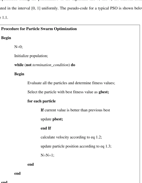
gbestare the best position found by the particle i so far and the best position found by the whole swarm so far respectively, ω is the inertia weight which determines how much the previous velocity is preserved. The parameters c1 and c2 are the cognitive and social parameters respectively which maintain the balance between the exploration and exploitation during the performance of the algorithm and r1 and r2 are random numbers generated in the interval [0, 1] uniformly. The pseudo-code for a typical PSO is shown below in Figure 1.1.Figure 1.1 Pseudo-code for a typical Particle Swarm Optimization algorithm. Procedure for Particle Swarm Optimization
Begin N=0;
Initialize population;
while (not termination_condition) do Begin
Evaluate all the particles and determine fitness values; Select the particle with best fitness value as gbest; for each particle
If current value is better than previous best update pbest;
end If
calculate velocity according to eq 1.2; update particle position according to eq 1.3; N=N+1;
end end end
5
Particle swarm optimization algorithms are widely preferred in the recent years over other evolutionary algorithms such as Genetic Algorithms (GAs). The main reasons for this are: PSO involves less number of parameters to adjust and it does not include removal of particles
from the population. It makes changes to the particles’ locations to arrive at the optimal solution.
Unlike GAs, PSO does not involve sharing of information through chromosomes. Only the location of the global best is shared among the particles through-out.
The efficiency of PSO is generally high compared to other evolutionary algorithms. PSO can locate significant optimal solution in a few function evaluations. This makes it more cost convenient.
The PSO has a flexibility to control the balance between global and local exploration of the search space. This unique feature enhances the search capability of the algorithm and avoids the problem of premature convergence thus making it more robust.
However, as always, there are drawbacks too, involved with PSO. Because of the stochastic nature of the algorithm, PSO does not always guarantee the finding of the optimal solution every single time. Also, because of the quicker convergence speed of the algorithm, in certain problem situations, the algorithm loses its diversity which impacts the performance of the algorithm negatively.
1.4 Research Goal and Approach
The goal of this thesis is to study and understand the behavior of dynamic optimization problem and its characteristics and design an algorithm that solves the problem with better accuracy, faster convergence and easier implementation. The proposed algorithm is a dynamic particle swarm optimization algorithm which involves multiple sub-swarms to locate the presence of multiple peaks. The algorithm also exploits information from the previous generations to adapt to the changes in the environment. The multiple swarms adapt to the new locations and help in
6
tracking the optimal solution. The algorithm is designed to have higher reusability, faster convergence, easier implementation, good accuracy and ability to work under severe and high frequency changes. The algorithm has been implemented on computer simulation program and tested on several benchmark test functions. The results are analyzed and compared to some of the state-of-the-art algorithms and found it competitive.
1.5 Document Organization
The rest of the document is organized as follows: In Chapter II, the dynamic optimization problems are discussed in detail. The chapter provides details about the dynamic optimization problem with respect to the aspects of changes that occur and the dynamic behavior of the fitness landscapes. The chapter provides a detailed literature survey of the dynamic evolutionary algorithms that have proposed so far by researchers for different problem settings and analyses their performance. In Chapter III, a dynamic particle swarm algorithm is proposed and analyzed. The proposed algorithm uses multiple swarms to identify multiple peaks and also uses information from the previous iterations to keep track of the particles’ behavior and tracks the optimal solution. In Chapter IV, the proposed algorithm is tested on several standard benchmark functions. The data obtained is analyzed and the results are discussed. Chapter V concludes the document with relevant observations and also recommends scope for future work.
7
CHAPTER II
DYNAMIC EVOLUTIONARY OPTIMIZATION
2.1 Introduction
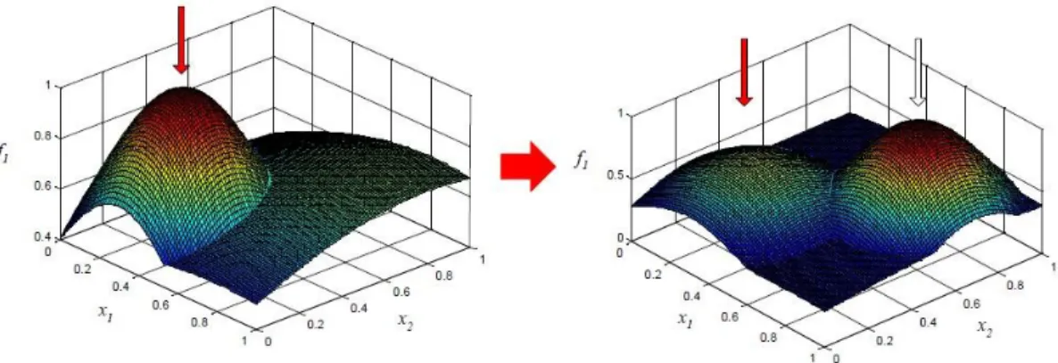
Many real world optimization problems are subject to changing conditions over time. These type of problems are termed as the dynamic optimization problems. The changes in the conditions include changes in the objective function, the problem instance, and/or constraints, etc., (see Figure 2.1). Consequently, the optimal solution of the problem under consideration changes reflecting to the changes in the conditions. These conditional changes could be reflected on the landscapes as changes in the optimal peak heights, shapes or locations or a combinations of these three [2].
Figure 2.1 Dynamic changes occurring in the fitness landscape
The challenges in solving these dynamic optimization problems arise from the occurrence of changes in the location, number and properties of the optimal solutions. When a standard
8
evolutionary algorithm converges under a certain problem setting, the diversity and exploration capacity of algorithm are greatly diminished. As a result, continuing the evolutionary process from the converged population without any further adaptation scheme to improve diversity or enhance the scope of exploration creates a higher probability of being unable to find the new optimal solutions or of being stuck with local optima. Therefore, it is very essential to implement certain scheme or mechanism in the evolutionary algorithm to account for the dynamism of the optimization problem.
There are several important aspects of dynamic optimization problems and these include severity, frequency, observability, detectability, and dynamics of change [3]. While higher severity of change necessitates the Dynamic Evolutionary Algorithm (DEA), to increase diversity and exploration, higher frequency of change requires a faster convergence after a change has occurred. If the severity of change is too high for the DEA, the algorithm may not locate the new optima or might get stuck in local optima. Similarly, if the frequency of change is faster than the adaptation speed of the DEA, the algorithm will not reach the optimal solutions before another change occurs.
In contrast to the above discussions, it is not always easy to detect a change unless it is observable. Some of the common ways followed by researchers include checking if the fitness of re-evaluated select individuals has changed significantly [3], checking if there is a significant change in the best fitness value found so far, etc. In most of the practices, it is also common to assume that a change is explicitly known to the system and the system has a built-in capacity to observe and detect changes instantly. In this thesis, it is assumed that change is explicitly known to the system.
In addition, DOPs may also involve different dynamic changes and these include constant, linear, circular/revolving, reshaping and random modes [3], [8], [9]. In majority of these cases,
9
the system dynamics is unknown and still the algorithm is expected to work without this knowledge. In this thesis, a dynamic particle swarm optimization is presented which adapts to the changes in the environment.
In general, a good DEA should be able to track and locate the optimal solution irrespective of the severity and frequency of change. It should overcome the loss of diversity and use a mechanism to enhance its exploration capacity. Coming to a case of a PSO, there is also another setback in the presence of dynamic environments which is the outdated memory. This means that there would be loss of information regarding the pbest and gbest. This, though not a serious issue compared to the diversity loss, is something which cannot be neglected either. Therefore, for a faster convergence and to re-diversify the population, it needs to use as much past information as possible to account for the lost memory as well. The extra computational cost incurred in this process should be justified with its performance improvement.
Some qualities sought in dynamic evolutionary algorithms include reusability, faster convergence, higher accuracy, faster adaptation, easier implementation, and better performance. Reusability is the ability of the algorithm to use as much information as possible from the previous iterations. Reusability enhances the convergence speed of the algorithm and quickly allows the algorithm to adapt to the new environment. When the severity of the change is high, it reduces the reusability of the data and requires higher exploration capability for the algorithm. Similarly, high frequency changes require faster convergence and adaptation. Accuracy is how close the found optimal solution is to the true optimum. Extra efforts to improve the accuracy may result in compromising with the convergence speed and therefore it is always important to maintain a delicate balance between the additional computational cost and the expected performance improvement. Adaptation, as the term suggests, refers to adapting the population to the new environment.
10
The algorithm proposed in this thesis achieves all the above qualities. The algorithm uses multiple swarms to track the behavior of the multiple peaks and uses a relocation principle, which involves relocation of individuals based on their previous evolutionary data which helps in maintaining the diversity. Since there is information from the past, the particles converge quickly to the new optimum. The use of multiple populations also helps in tracking the optima even for severe or drastic changes. The relocation data used is specific to every particle and thus gives better adaptation to the population in contrast to the algorithms that use a single adaptation scheme for every particle. As a result, there is a significant progress in the evolutionary process giving faster adaptation, better accuracy, and quicker convergence to the algorithm.
The rest of the chapter is organized as follows; Section 2.2 provides a brief summary of the different types of fitness landscapes. Section 2.3 explains about the various characteristics of the dynamics involved in the DOPs. Section 2.4 gives a detailed explanation of the various evolutionary approaches proposed by researchers so far to tackle the DOPs. In Section 2.5, few of the performance metrics that are used to compare optimization approaches have been discussed in detail. The various types of benchmark test functions which are used to test the behavior of the algorithms are discussed in Section 2.6. Finally, the chapter is concluded with a brief summary in Section 2.7.
2.2 Types of Fitness Landscapes
Depending on the changes over the landscapes through time, Weicker et al [9] classified fitness landscapes into different categories. Firstly, stationary or static landscapes where there is no change or movement in the landscapes. These are most commonly used for EA studies. The second type of fitness landscapes are the ones that change constantly every period of time. The dynamic optimization algorithm is expected to estimate the recurrent amount of change and adapt accordingly after a few iterations. These are relatively easy to implement and pose very small
11
difficulty for the algorithm. The next category of fitness landscapes has periodic changes. Here, the landscape changes to its original state after a few change cycles. The difficulty lies in predicting the time period for these periodic changes which is difficult for the algorithm to react. Generally algorithms are designed to have a small memory element to store a few past locations of the optimum for a possible re-use in these types of situations. The fourth type of fitness landscapes is termed as homogeneous landscape where the entire landscape moves coherently as opposed to various parts behaving heterogeneously. The fifth and last category of fitness landscapes is called alternating landscapes where the optimum moves from one peak to another. The changes occurring in the landscape are completely random and stochastic in nature. These type of problems are the most difficult ones for the algorithm to tackle as there is no consistent behavior in terms of the occurrence of change. Hence, implementing a proper adaptation scheme in the algorithm is very much necessary to cope with dynamic nature of the landscape.
Figure 2.2 Dynamic Fitness Landscape 2.3 Characteristics of Dynamic Optimization Problems
It has to be understood that whenever a change occurs in the environment, it has to be within the exploitation limits of the algorithm to perform an adaptation scheme for the population. On
12
the other hand, if a problem changes drastically without any exploitable similarities, it could be regarded as two independent problems and the algorithm needs to be started from scratch as there would be no useful historic data. For this reason, we pertain our studies only to the systems where the dynamic changes in the environment have a significant amount of historic information from the past environmental state that could be exploited after the occurrence of change.
As discussed earlier, it is very important to first understand the several characteristics of change and the important aspects of DOPs in further detail before learning about the approaches and the benchmark test functions. Several such important characteristics and aspects of the DOPs exist which are worth a mention here. These include severity, frequency, observability, detectability and dynamics of change [3]. This section sheds light on these aspects in some details.
2.3.1 Severity of change – Severity of change refers to the amount or magnitude of the change that has occurred in the landscape. The higher the severity, the lesser is the correlation of the new landscape with the previous one and therefore, this requires the algorithm to enhance the diversity and exploration. Sometimes very severe changes may result in the algorithm failure to locate the optima. Therefore, it is very much essential to have an algorithm that performs well under drastic changes.
2.3.2 Frequency of change – The frequency of change indicates how quickly the landscape changes occur. A high frequency requires the algorithm to converge faster and locate the optima before there is another change in the landscape. Very high frequencies are difficult to tackle because the landscape changes even before the algorithm converges. Hence, a good algorithm should have high adaptation frequency and faster convergence.
2.3.3 Observability and Detectability – These two closely related characteristics seem pretty simple to understand but they are very important aspects to be kept in mind while designing a
13
dynamic evolutionary algorithm. Most of the time it is assumed that any change occurring in the landscape can be observed and detected which is not true. Several methods have been proposed in literature to detect these changes (e.g., [10]). Some of the methods detect the changes by re-evaluating a select population of individuals and checking whether their fitness has changes significantly or not. It is also a common practice to assume that the occurrence of change is known to the system and these changes can be detected instantly. This helps the researchers to focus solely on the design of the algorithm.
2.3.4 Dynamics of change – This represents the way the landscape moves when a change has
occurred. A reshaping dynamics has a landscape that changes it morphology on the occurrence of change. A sliding or drifting dynamics results in the drifting of the optima in the landscape. A periodic or oscillatory dynamics causes the optima to change periodically. A random or stochastic dynamics has the optimum that changes randomly. In all these cases, the type of the dynamics is not explicitly known to the system and the algorithm is expected to work irrespectively.
2.4 Literature Review
Several researchers have focused on the DOPs over the last couple of decades and there are multiple approaches that have been proposed to handle the DOPs. Recently Branke et al [1] classified the different types of approaches used by researchers so far. These categorizations provide some interesting insights on the current trend of literature and the proportion of studies with respect to the approaches in each category. Each category has been explained below with few examples from the literature along with their advantages and drawbacks. For more detailed reviews, readers are referred to the references cited in [1] and [2].
2.4.1 Introducing Diversity – The main problem in designing a dynamic evolutionary algorithm is the issue of diversity loss. From the discussions in the thesis so far, it is pretty evident that the algorithm loses its diversity after converging at the optimum before the
14
occurrence of a change. Therefore, it is very important to induce diversity into the population after a change has occurred.
Re-initialization of the population to induce diversity has been the most naïve approach ever. Many algorithms and variations of the standard evolutionary algorithms are proposed with different modifications and methodologies of re-initialization [2]. One general idea that comes to one’s mind when thinking about re-initialization is to randomly re-initialize the population once again after the occurrence of change. But it has to be noted that this type of re-initialization causes a loss of historic information from the previous iterations and is therefore generally not preferred.
In a typical GA, one approach to enhance diversity has been introducing an adaptive mutation parameter call hyper-mutation, proposed by Cobb [13], in which the mutation rate is a multiplication of the normal mutation rate and a hyper-mutation factor. This hyper-mutation is invoked after the occurrence of a change. This concept of inducing diversity after the occurrence of a change has been implemented in a PSO by Hu and Eberhart in [12], in which a part of the swarm or whole swarm will be re-diversified using randomization. Daneshyari and Yen [11] proposed a cultural-based PSO where the framework of knowledge inspired from belief space in Cultural Algorithms is used to re-diversify the population after a change has occurred.
Woldesenbet and Yen [14] proposed a new method of re-initialization using the concept of variable relocation where the sensitivity of the individuals for the changes in the environment is calculated to estimate the specific relocation radius for the particles. Sensitive individuals have larger relocation radii. In this thesis, the similar concept is applied to a PSO by measuring the sensitivity of the particles for changes in the environment and calculating the relocation radii for the particles after a change has occurred.
15
In these types of methods, since there is no computation involved in maintaining the diversity all through the process, the algorithm can completely focus on the search process alone. In addition, these methods resembles a type of local search which helps in exploiting the nearby places of the optimum. However, the drawbacks of this approach include dependency on the knowledge of the occurrence of change which is really difficult. Also, it is always not very easy to know the correct values of mutation parameters and once the algorithm converges, only the knowledge of the optimum is known whereas a lot more could be relevant.
2.4.2 Maintaining diversity – From the above approaches it can be understood that the maintenance of diversity is a very important part of the dynamic evolutionary algorithm. Apart from introducing the diversity after the occurrence of change, diversity can also be maintained through-out the process of the algorithm. The main idea behind this approach is to avoid premature convergence of the algorithm. Grefenstette [15] proposed a method called Random Immigrants in which new individuals are added at random locations to the population for every generation. The addition of new individuals brings more diversity to the total population. But it has to be kept in mind that this also constantly increases the population size.
In another approach, Yang and Yao [42] proposed Population-based Incremental Learning (PBIL) approach in which the algorithm uses a probability vector to generate the individuals in the population. The probability adapts according to the best solution in each generation. Blackwell et al. [16] proposed a variation of the PSO, called the charged PSO, in which a repulsion mechanism is applied. Inspired from the concept of atoms in an electric field, the algorithm prevents particles from getting too close to each other. Bui et al. [17] used a multi-objective strategy where first multi-objective is the original multi-objective which is to search for the optimum whereas the second objective is created for maintaining the diversity during the course of the algorithm.
16
Many approaches have been proposed to maintain the diversity within the algorithm and they all show that the respective algorithm works great for solving problems because of their respective diversity maintenance strategies. The idea of maintaining diversity during the run of the algorithm may be good for solving problems with severe changes and environments with rare changes. However, if the changes are small, addition of individuals might create too much diversity and effect the convergence of the algorithm. Also, using such complex strategies to focus continuously on diversity may slow down the convergence process.
2.4.3 Memory Approaches – In this type of approaches, the algorithm is provided with some kind of memory that allows it to store optimal solutions and reuse them at a later stage when required. This could be done implicitly by using some redundant representation or explicitly by including an external memory component and employing strategies to store, update and retrieve information from this memory element. Strategies with a memory are very useful in environments when the environment changes periodically, when there are repeated occurrences of a set of conditions. In addition, redundant representations might slow down the process of convergence but they could favor diversity.
Implicit approaches use a built-in form of implicit memory in the algorithm. One such form if implicit memory is the redundant representation and diploidy is one common approach [19]. A diploid algorithm is one which contains two alleles at each locus. Usually GAs are haploid for static optimization problems, but it is believed that using diploid or multi-ploid approaches could be useful in solving the dynamic optimization problems. Smith and Goldberg [20, 21] employed a tri-allelic scheme in which an allele could take any one of the three possible values “0”, “1 recessive”, and “1 dominant”.
The explicit memory approaches include an external memory component to store the best results and these are added back to the population if they are better fit than the current population.
17
Algorithms following this approach need to follow four aspects. First, the algorithm has to decide on the content of the memory, like what to store and what not to store. In general previous best solutions or local optima are stored in the memory [22]. In [23], the most diversified solutions, in terms of standard deviations, are stored. In [11], the set of previous solutions along with the locations of each individual are saved in the memory.
The next aspect is how to update the memory. In most cases, the best found elements of the current generation will replace the old values in the memory. The elements that are removed are the oldest members in the memory or ones with least contribution to the diversity of the population or individuals with least contribution to fitness or a combination of these. The next aspect is when to update the memory. Ideally, it should happen after the occurrence of a change. But practically, detecting or observing a change at the time of its occurrence is very difficult. Therefore, algorithms generally update their memory after every iteration or after a specific number of iterations. The final aspect to focus on is how to use the memory. Generally the best individuals stored in the memory are used to replace the worst individuals in the population. This replacement happens after every iteration or after a specific number of iterations. It could also be done after the detection of change if the change could be detected.
These memory based approaches are effective for solving problems that are set up in cyclic environments. Due to their ability to retrieve previous best solutions from the memory, these approaches are quite suitable for periodic and cyclic environments. However, these seem to be effective only if the environment is either cyclic or periodic in nature and the memory becomes obsolete when the environment changes are not cyclic [3]. Apart from the problems like convergence and diversity, these approaches also incur problems due to their memory elements. The redundant approaches might not be effective if the periodicity of the environment is too large. As pointed out by Branke in [3], these approaches sometimes are not good enough to maintain the diversity of the algorithm.
18
2.4.4 Multi-population approaches – This type of approach, as the name suggests, involves more than one population in the algorithm. Generally, the total population is divided into two groups where one looks for the optima and the other tracks the changes in the environment. In general there is one main population and one group of sub-populations or “child populations.” The idea behind using this approach is that the main population tracks the location of the optima while the child population or sub-population looks out for any changes in the environment. Oppacher and Wineberg [25] proposed a method which they called the shifting balance genetic algorithm, which uses one main population to exploit the best optimum and several small colonies to explore the search space.
Ursem [28] proposed another multi-population approach called the multinational GA in which the grouping of individuals is done based on “hill-valley detection procedure.” Here, two points are selected in the search space and a valley is assumed if the fitness at a sample point between those two points is less than both the end points. The drawback with this approach is that it involves numerous function evaluations just for the detection of a valley. Another method proposed in [26] by Branke et al., called the Self-Organizing Scouts (SOS), uses a main large population to search for the optima and dedicates several small populations to track any changes in the optimum that has been found so far by the algorithm. A small population is created whenever the main population finds a new optimum location. In the above approaches the population sizes of parent and child populations is adjusted depending on the performance of the algorithm.
One more approach is giving equal importance to both the populations. In this type both the populations search for the optimum in the search space and also simultaneously track changes in the environment. Kennedy [43] proposed a variation of PSO which uses a k-means algorithm to locate the centers of different clusters of the particles in the population. Then these centers are used to substitute the pbest or gbest locations. The k-means algorithm is run thrice to stabilize the
19
cluster centers. But the limitation that lies here is choosing the number of clusters. One other example is the Speciation PSO (SPSO) [29], proposed by Parrott and Li, where each sub-population is a hyper-sphere defined by the best fit individual and a specific radius. In this case, there is an overlap of particles in the search space which leads to a loss in the diversity. Clustering approaches help in having multiple populations while maintaining diversity during the evolutionary process of the algorithm. Yang and Li [30] proposed an adaptive approach called the Clustering Particle Swarm Optimization (CPSO) where a clustering mechanism is used to maintain diversity during the course of the algorithm.
The multi-population approaches can maintain the diversity though the run of the algorithm. They can recall some information from the past generations and the existence of multi-populations also helps in tracking the presence of multiple optima and also can be effective for solving problems with competing peaks or multi-modal problems. However, it is difficult to determine the number of sub-populations, the search space for each population, the population size etc. In CPSO [30], an adaptation strategy and clustering principle is used to determine the number of sub-populations depending on the landscape settings.
In the recent years, multi-population approaches have gained importance for solving DOPs due to their diversity enhancing capability and the ability to track the presence of multiple optima. Recently a generic framework for solving DOPs using multiple swarms was proposed by Yang and Li [27]. In this thesis, we follow the framework described in [27] to form sub-populations and then use a relocation strategy to replace the particles after the occurrence of a change.
2.4.5 Self-Adaptation and Mutation – The self-adaptation mechanism is an outcome of a process which involves learning and predicting based on historic data. When a change occurs, the population undergoes a transient state where the values of the operators are changed to enhance diversity and performance of the algorithm. In [9], several self-adaptation schemes are compared.
20
Cobb and Grefenstette [31] introduced the idea of hyper-mutation in which mutation probability is increased after a change has occurred. Ursem [28] proposed a Multinational Genetic Algorithm (MGA) in which five different parameters are encoded in the genomes of the MGA for adaptation. Other suggested techniques include life-time learning [32] and adaptive chaotic mutation [33].
The assumption in this type of approaches is that the occurring environmental changes are in the reach of the algorithm’s adaptation capability. Otherwise, the adapted population would be inefficient and might not locate the new optimal solution.
2.5 Performance Metrics
There are several performance indexes that have been proposed so far for measuring the performance of dynamic evolutionary algorithms. In this thesis, we have used offline error performance [34] and adaptation performance [35] for measuring the performance of the proposed dynamic evolutionary algorithms.
2.5.1 Offline error performance – Off-line error performance index [34] is the most common performance index used by researchers recently. It is obtained as the average of the error between the true optimal point and the best fitness at each evaluation. This can be mathematically expressed as:
T i i best true avg offlinef
f
T
e
1)
(
1
(2.1)where i is the evaluation counter; T is the total number of evaluations considered; ftrueis the true optimum solution after the occurrence of a change; and finally fibest is the fitness value of the best particle until the current iteration after the occurrence of the change. This form of performance evaluation of an algorithm is helpful in evaluating the overall performance of an algorithm and to
21
compare the final outcomes of different algorithms. However, there are certain disadvantages. One is that they require that the time of the occurrence of change has to be known and the other is that these measures are not normalized and therefore, there arise a possibility of the values becoming biased under certain specific circumstances.
2.5.2 Adaptation performance – Adaptation performance [35] is the average ratio between the best fitness value and the true optimum at each iteration. This can be mathematically expressed as:
T i true bestf
f
T
I
11
(2.2)where i is the evaluation counter; T is the total number of evaluations considered; ftrueis the new true optimum solution which is updated after the occurrence of a change; and fbest is the fitness value of the best particle until the current iteration after the occurrence of a change. This gives a measure of the adaptation capability of the algorithm. But however, this way of formulating the error is not a good indication for measuring the performance when the fitness functional values are very small.
2.6 Benchmark problems for Dynamic Evolutionary Algorithms
In the past few years, researchers have proposed several benchmark test functions for the purpose of testing the performance of the proposed evolutionary algorithms. In general, these test functions simulate the behavior of real world optimization problems and provide a simple mechanism to control the landscape dynamics.
A good benchmark function should be flexible, simple and efficient. It should be flexible to incorporate all the dynamics of the real world optimization problem with different dynamic settings and scales. It should be simple enough to be implemented and analyzed and it should be
22
computationally efficient. And most importantly it should allow conjectures to real-world problems or resemble them to as much extent as possible [3].
The earliest forms of dynamic optimization test problems use a number of standard static optimization problems and switch back and forth between these landscapes through the run of the algorithm [31]. Other forms of dynamic functions use a number of peaks that are independent of each other and are specified by their height, width and location. Branke [37] proposed a general platform for such kind of problems called the Moving Peaks Benchmark (MPB) Problem which has been widely used in the literature in the recent years. Within the problem setting of the MPB problem, the optima can be varied by changing the location, height and width of the peaks. It can be mathematically expressed as:
)))
(
),
(
),
(
,
(
max
),
(
max(
)
,
(
,..., 1 1P
x
h
t
w
t
p
t
x
B
t
x
F
i i i M
(2.3)where B(x)is a time-invariant landscape and P is the function defining the peak shape, where each of the M peaks has its own time-varying parameters: height (h), width (w) and location
)). (
(pi t The different shapes of the peaks determine the type of the test function. When the peaks have a cone shape, it becomes competing cones problem [38] and on the other hand, if the peaks have a ‘Gaussian’ shape, then it becomes time-varying Gaussian peaks problem [39].
The most frequently used test function by researchers is the competing cones problem
proposed by Morrison and de Jong [38]. It consists of a number of cones each independently defined by height, center and width. The cones are non-differentiable at their peaks and give a good justification for real world optimization problems. It is expressed mathematically as:
n j ij j i i M iH
R
x
X
x
f
1 2 ,..., 1(
)
max
)
(
(2.4)23 where x (x1,x2,....,xn)
is a point in the landscape, M is the number of cones that are present in the environment, and each cone i is independently described by its height Hi, slope Ri, and its center
X
i
(
X
i1,....,
X
iM).
One more commonly used test function in recent times is the Gaussian peaks problem which was proposed by Grefenstette [39]. This is very much similar to the moving cones problem explained above except for the shape of the peaks. The peaks have a ‘Gaussian’ shape in contrast to the cone shape above. The peaks are non-differentiable at their vertex and this problem provides a good benchmark for evaluating dynamic optimization problems. However, this becomes quite challenging when the number of peaks is very high. It can be mathematically expressed as . ) ( 2 )) ( , ( exp ) ( max ) , ( 2 2 ,.. 1 t t C X d t A t X f i i i N i
(2.5)where Ai(t)is the amplitude, Ci(t)denotes the center and
i(t)represents the width of the n-dimensional Gaussian peak.There are other forms of test functions that are common shift stationary optimization test problems using various dynamics of change. One good example of this type is the moving parabola problem [40, 41]. The general form of the objective in this problem is given mathematically as
.
))
(
(
)
,
(
1 2
n i it
x
Min
t
x
f
(2.6)The amount of shift in the landscape,
i(t), can have different dynamics of change and the general types are linear, random and circular dynamics of change. Another interesting function24
that was used by Branke in [8] is called the Oscillating peaks function. There are l landscapes each consisting of m randomly chosen peaks similar to the moving peaks benchmark problem. Each of these landscapes oscillate according to a cosine function. As a result of this oscillation, the optima also oscillates between different points. This is given mathematically as
. 5 . 0 ) 1 2 2 cos( 5 . 0 ) ( )) 0 ( ), ( ( ) ( l i steps t t w f t w Max t fi i
(2.7) 2.7 SummaryThe above sections give an understanding about the dynamic optimization problems and show the different approaches that have been proposed so far. The strengths and weaknesses of all the approaches are discussed in detail and gives a clear understanding of the problem settings and the approaches. The chapter also discusses few benchmark problems that have been used in this document along with a couple of performance metrics that are used in this thesis.
25
CHAPTER III
PROPOSED DYNAMIC PARTICLE SWARM OPTIMIZATION
The proposed algorithm adopts the general framework of using multi-swarms with clustering [27] to create adaptable multiple sub-swarms and then exploit the previous history of the best particles’ location and adapt the current location according to the environmental changes. The algorithm uses clustering technique to create sub-swarms to explore the different areas and peaks in the search space and after the occurrence of a change, the algorithm measures the particles’ sensitivity to the environmental changes and shifts the particle in the decision space by a so-called relocation radius [14] which is determined based on the estimate of the environmental change that has occurred. The algorithm is explained in detail below.
Let f=f(X,e) be the DOP we would like to optimize, where X represents the D-dimensional decision space vector and xd is the dth-dimensional decision variable. For the purpose of this document, the optimization problem is assumed to be a minimization problem. It needs to be noted that a maximization problem can be converted to a minimization problem by multiplying the objective function with -1 (i.e. duality principle).
3.1 Creating Multiple sub-swarms
Though there are several multi-population approaches proposed in literature, Clustering Particle Swarm Optimization [30] seems to be a competitive one as it alleviates the general problems faced by other multi-swarm approaches. The proposed algorithm, inspired from CPSO, uses a single linkage hierarchical clustering scheme to form clusters. The distance between two
26
individual particles i and j in the d-dimensional space is given by their Euclidean distance which is calculated as
D d d j d ix
x
j
i
d
1 2)
(
)
,
(
(3.1)Given an initial population pop, the clustering algorithm first creates a list G of clusters containing only one particle. Then it uses a specific algorithm called FindNearestPair to find a pair of clusters t and s such that they are the closest among all the clusters in G. If the total number of particles in both clusters is less than a predefined maximum sub-population size, called
subSize, both clusters t and s are combined into one cluster. This process is continued until all the clusters in G have more than one single particle. The cluster list G thus created is appended to a sub-population list plst.
The distance between two clusters t and s in the list G, is denoted by M(t, s), is defined as the closest distance between two individual particles i and j which belong to the two clusters t and s
respectively. M(t, s) is mathematically calculated according to the Equation 3.2 given below.
)
,
(
min
)
,
(
,d
i
j
s
t
M
s j t i
(3.2)It can be observed from the above description, that the clustering process adaptively creates sub-swarms depending on the distribution of the particles in the fitness landscape. The number of sub-swarms and the size of each swarm are automatically determined by the algorithm and the parameter subSize. The pseudo-code for the overall clustering process is described in Figure 3.1 and Figure 3.2.
27
Figure 3.1 Pseudo-code for the Clustering Algorithm to form sub-swarms. Procedure: Clustering
Begin
Create a temporary cluster list G of size [pop]; for each individual particle i in popdo
G[i] = pop[i]; (each cluster has one particle) end for
Calculate the distance between all clusters in G and construct a distance matrix M of size |G|×|G|;
while TRUE do
if !FindNearestPair then Break;
end if
t=t+s; (Merge clusters t and s) Delete cluster s from G;
Recalculate all distances in M that are affected because of the merging of t
and s;
if every cluster in G has more than one particle then Break; end if end while Remove pop; plst = plst + G; end
28
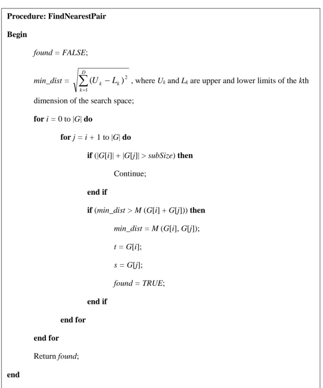
Figure 3.2 Pseudo-code for FindNearestPair Algorithm Procedure: FindNearestPair Begin found = FALSE; min_dist =
D k k kL
U
1 2)
(
, where Ukand Lkare upper and lower limits of the kth dimension of the search space;for i = 0 to |G| do for j = i + 1 to |G| do if (|G[i]| + |G[j]| > subSize) then Continue; end if if (min_dist > M (G[i] + G[j])) then min_dist = M (G[i], G[j]); t = G[i]; s = G[j]; found = TRUE; end if end for end for Return found; end
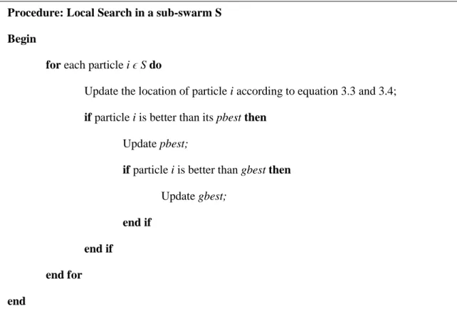
29 3.2 Local Search Strategy
Once the sub-swarms are created using the above shown clustering method, local search is performed by each sub-swarm in its sub-region of the search space. Each sub-swarms works independently and there is no sharing of information among the swarms. This gives the algorithm an opportunity to explore different areas of the search space and helps in tracking multiple peaks in the landscape. In order for a sub-swarm to locate a local peak, the general particle swarm optimization approach (discussed earlier) is implemented.
)
(
)
(
, 2 2 1 1 d i d gbest d i d pbest i d i rd iv
c
r
x
x
c
r
x
x
v
(3.3) rd i d i rd ix
v
x
(3.4)To enhance the speed of the convergence process, the inertia weight ω is varied dynamically according to Equation 3.5. This parameter, along with c1and c2 (cognitive and social parameters, respectively), control the balance between exploration and exploitation in a traditional PSO. The value of this inertia weight is generally chosen as 0.9. But it makes sense to have a large value during the initial iterations to enhance the exploration and then decrease it gradually to favor more on exploitation. It is therefore decreased linearly according to the following equation,
,
_
)
(
max min maxiter
total
iter
(3.5)where
minand
maxare the minimum and maximum limits for the parameter
,iter is the current count of iterations and total_iter is the total number of iterations of the algorithm.30
Figure 3.3 Pseudo-code for performing the local search in a sub-swarm S. 3.3 Redundancy Control
Redundancy control is to remove the redundant particles in the population. This includes particles that are converged, overcrowded particles in a sub-region and particles located in the overlapping region of two sub-populations. It is very essential to perform this redundancy check because, firstly, these particles do not contribute to the search progress and secondly, it is a waste of computational resources to perform unprofitable evaluations on these particles.
To perform an overlap check between two populations, the concept of search radius is introduced. The search radius of a population is defined as average distance of every particle in the population to the central particle of the population. It can be mathematically represented as
Procedure: Local Search in a sub-swarm S Begin
for each particle i ϵ S do
Update the location of particle i according to equation 3.3 and 3.4; if particle i is better than its pbestthen
Update pbest;
if particle i is better than gbest then Update gbest;
end if end if
end for end
31
,
)
,
(
1
)
(
s i centers
i
d
s
s
radius
(3.6)where scenter is the central position of the sub-population s and |s| is its population size. If any particle of a sub-population lies within the search radius of another sub-population then it is said that overlapping occurred. If the distance between the best particles of two sub-populations is less than their search radius then they are combined or one of them is removed. It is generally assumed that one sub-population covers one peak but however, it may not be always true. If a sub-population covers more than one peak, other sub-populations within its search area should not be removed because there is a possibility of losing those peaks. This has to be taken into consideration before combining two overlapping populations.
Therefore, before combining two populations, t and s, which are within each other’s search
radius, an overlap ratio, roverlap(t, s) is calculated. The populations are merged only if this overlap ratio is larger than a preset threshold value of β. The percentage of particles from s within the search radius of t and the percentage of particles from t within the search radius of s is calculated and the lowest of these values is chosen as the overlap ratio between the two populations. It has to be noted that the radius used in the above calculation is the radius calculated when the sub-swarms are formed. The reason for this is that it gives a quicker identification of the overlap.
In order to avoid too many particles searching for a single peak, and overcrowding check needs to be performed on each sub-population after the overlapping check. If the number of particles in a sub-population is greater than subSize then those extra particles are removed from the population to equate the population size to subSize. In addition to this, a converged sub-population does not yield any result to the search progress. Therefore, it is beneficial to remove these individuals from the population. If the radius of a sub-population is smaller than a threshold value ε, which is selected as 0.01, then the population can be considered as converged. These
32
individuals are removed from the sub-population list plst. The pseudo-code for the redundancy control is given in Figure 3.4.
Figure 3.4 Pseudo-code for performing Redundancy Control. Procedure: Redundancy Control
Begin
for each pair of sub-populations (t, s) in plstdo if roverlap(t, s) > β then
Merge t and s into t; Remove s from plst; end if
end for
for each sub-population t ϵ plst do if |t| > subSize then
Remove worst (|t| - subSize) individuals from t; end if
end for
for each sub-population s ϵ plst do if radius(s) < ε then
Remove s from plst; end if
end for end
Update the location of particle i according to equation 3.3 and 3.4; if particle i is better than its pbestthen
Update pbest;
if particle i is better than gbest then Update gbest;