Optimization: Convergence, Complexity
and Applications
Shiqian Ma
Submitted in partial fulfillment of the
requirements for the degree of
Doctor of Philosophy
in the Graduate School of Arts and Sciences
COLUMBIA UNIVERSITY
2011
Shiqian Ma All Rights Reserved
Algorithms for Sparse and Low-Rank Optimization: Convergence, Complexity and Applications
Shiqian Ma
Solving optimization problems with sparse or low-rank optimal solutions has been an important topic since the recent emergence of compressed sensing and its matrix extensions such as the matrix rank minimization and robust principal component analysis problems. Compressed sensing enables one to recover a signal or image with fewer observations than the “length” of the signal or image, and thus provides potential breakthroughs in appli-cations where data acquisition is costly. However, the potential impact of compressed sensing cannot be realized without efficient optimization algorithms that can handle ex-tremely large-scale and dense data from real applications. Although the convex relaxations of these problems can be reformulated as either linear programming, second-order cone programming or semidefinite programming problems, the standard methods for solving these relaxations are not applicable because the problems are usually of huge size and con-tain dense data. In this dissertation, we give efficient algorithms for solving these “sparse” optimization problems and analyze the convergence and iteration complexity properties of these algorithms.
Chapter 2 presents algorithms for solving the linearly constrained matrix rank mini-mization problem. The tightest convex relaxation of this problem is the linearly constrained nuclear norm minimization. Although the latter can be cast and solved as a semidefinite
are large. In Chapter 2, we propose fixed-point and Bregman iterative algorithms for solv-ing the nuclear norm minimization problem and prove convergence of the first of these algorithms. By using a homotopy approach together with an approximate singular value decomposition procedure, we get a very fast, robust and powerful algorithm, which we call FPCA (Fixed Point Continuation with Approximate SVD), that can solve very large matrix rank minimization problems. Our numerical results on randomly generated and real matrix completion problems demonstrate that this algorithm is much faster and provides much better recoverability than semidefinite programming solvers such as SDPT3. For example, our algorithm can recover 1000×1000 matrices of rank 50 with a relative error of 10−5in about 3 minutes by sampling only 20 percent of the elements. We know of no other method that achieves as good recoverability. Numerical experiments on online recommendation, DNA microarray data set and image inpainting problems demonstrate the effectiveness of our algorithms.
In Chapter 3, we study the convergence/recoverability properties of the fixed-point con-tinuation algorithm and its variants for matrix rank minimization. Heuristics for determin-ing the rank of the matrix when its true rank is not known are also proposed. Some of these algorithms are closely related to greedy algorithms in compressed sensing. Numer-ical results for these algorithms for solving linearly constrained matrix rank minimization problems are reported.
Chapters 4 and 5 considers alternating direction type methods for solving composite convex optimization problems. We present in Chapter 4 alternating linearization algorithms
the sum of two convex functions. Our basic methods require at most O(1/ε) iterations to obtain an ε-optimal solution, while our accelerated (i.e., fast) versions require at most
O(1/√ε) iterations, with little change in the computational effort required at each iter-ation. For more general problem, i.e., minimizing the sum of K convex functions, we propose multiple-splitting algorithms for solving them. We propose both basic and accel-erated algorithms withO(1/ε)andO(1/√ε)iteration complexity bounds for obtaining an ε-optimal solution. To the best of our knowledge, the complexity results presented in these two chapters are the first ones of this type that have been given for splitting and alternating direction type methods. Numerical results on various applications in sparse and low-rank optimization, including compressed sensing, matrix completion, image deblurring, robust principal component analysis, are reported to demonstrate the efficiency of our methods.
List of Figures iv
List of Tables vii
Acknowledgements ix
1 Introduction 1
1.1 Background and Motivation . . . 1
1.2 Preliminaries . . . 2
1.2.1 Basic Notation . . . 2
1.2.2 Sparse and Low-Rank Optimization . . . 4
1.2.3 Iteration Complexity and Alternating Direction Methods . . . 8
2 Fixed Point and Bregman Iterative Methods for Matrix Rank Minimization 13 2.1 Introduction . . . 13
2.2 Fixed-point iterative algorithm . . . 20
2.3 Convergence results . . . 26
2.4.1 Continuation . . . 33
2.4.2 Stopping criteria for inner iterations . . . 33
2.4.3 Debiasing . . . 34
2.5 Bregman iterative algorithm . . . 35
2.6 An approximate SVD based FPC algorithm: FPCA . . . 39
2.7 Numerical results . . . 42
2.7.1 FPC and Bregman iterative algorithms for random matrices . . . 43
2.7.2 Comparison of FPCA and SVT . . . 48
2.7.3 Results for real data matrices . . . 51
2.8 Conclusion . . . 56
3 Convergence and Recoverability of FPCA and Its Variants 58 3.1 Introduction . . . 58
3.2 Restricted Isometry Property . . . 60
3.3 Iterative Hard Thresholding . . . 67
3.4 Iterative Hard Thresholding with Matrix Shrinkage . . . 75
3.5 FPCA with Given Rankr . . . 78
3.6 Practical Issues . . . 81
3.7 Numerical Experiments . . . 83
3.7.1 Randomly Created Test Problems . . . 83
3.7.2 A Video Compression Problem . . . 88
vex Functions 92
4.1 Introduction . . . 92
4.2 Alternating Linearization Methods . . . 100
4.3 Fast Alternating Linearization Methods . . . 106
4.4 Comparison of ALM, FALM, ISTA, FISTA, SADAL and SALSA . . . 111
4.5 Applications . . . 116
4.5.1 Applications in Robust Principal Component Analysis . . . 118
4.5.2 RPCA with Missing Data . . . 121
4.5.3 Numerical Results on RPCA Problems . . . 123
4.6 Conclusion . . . 127
5 Fast Multiple Splitting Algorithms for Convex Optimization 129 5.1 Introduction . . . 129
5.2 A class of multiple-splitting algorithms . . . 134
5.3 A class of fast multiple-splitting algorithms . . . 142
5.3.1 A variant of the fast multiple-splitting algorithm . . . 148
5.4 Numerical experiments . . . 150
5.4.1 The Fermat-Weber problem . . . 150
5.4.2 An image deblurring problem . . . 154
5.5 Conclusions . . . 162
6 Conclusions 165
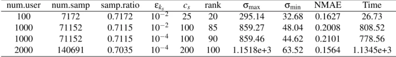
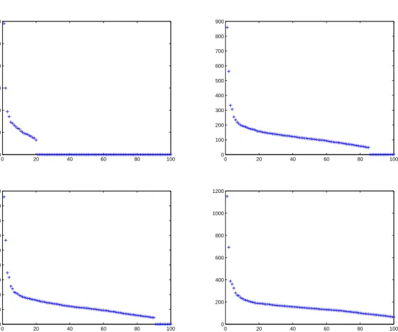
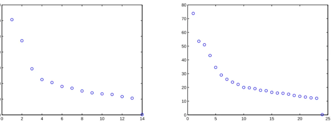
2.1 Distribution of the singular values of the recovered matrices for the Jester data set using FPC1. Left:100 users, Middle: 1000 users, Right: 2000 users 52 2.2 Distribution of the singular values of the recovered matrices for the Jester
data set using FPCA. Upper Left: 100 users, εks =10−2,cs =25; Upper
Right: 1000 users, εks =10
−2,c
s =100; Bottom Left: 1000 users, εks =
10−4,cs=100; Bottom Right: 2000 users,εks=10−
4,c
s=200 . . . 53
2.3 Distribution of the singular values of the matrices in the original DNA mi-croarray data sets. Left: Elutriation matrix; Right: Cdc15 matrix. . . 55 2.4 (a): Original 512×512 image with full rank; (b): Original image truncated
to be of rank 40; (c): 50% randomly masked original image; (d): Recovered image from 50% randomly masked original image (rel.err =8.41e−2); (e): 50% randomly masked rank 40 image; (f): Recovered image from 50% randomly masked rank 40 image (rel.err=3.61e−2); (g): Deter-ministically masked rank 40 image (SR = 0.96); (h): Recovered image from deterministically masked rank 40 image (rel.err=1.70e−2). . . 57
rank equaled 2 . . . 86 3.2 Comparison of frames 4, 12 and 18 of (a) the original video, (b) the best
rank-5 approximation and (c) the matrix recovered by FPCA . . . 91
4.1 Comparison of the algorithms . . . 117 4.2 In the first 3 columns: (a) Video sequence. (b) Static background recovered
by our ALM. Note that the man who kept still in the 200 frames stays as in the background. (c) Moving foreground recovered by our ALM. In the last 3 columns: (a) Video sequence. (b) Static background recovered by our ALM. (c) Moving foreground recovered by our ALM. . . 126
5.1 Comparison of MSA, FaMSA-s and Grad for differentµ. . . 160 5.2 Using MSA to solve (5.4.7). (a): Original image; (b): Blurred image; (c):
Reconstructed image by MSA . . . 161
2.1 Parameters in Algorithm FPC . . . 44
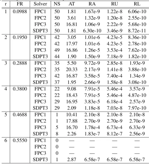
2.2 Comparisons of FPC1, FPC2, FPC3 and SDPT3 for randomly created small matrix completion problems (m=n=40, p=800, SR=0.5) . . . 45
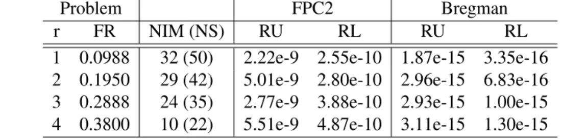
2.3 Numerical results for the Bregman iterative method for small matrix com-pletion problems (m=n=40, p=800, SR=0.5) . . . 46
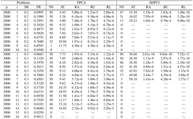
2.4 Numerical results for FPCA and SDPT3 for randomly created small matrix completion problems (m=n=40, p=800, SR=0.5) . . . 48
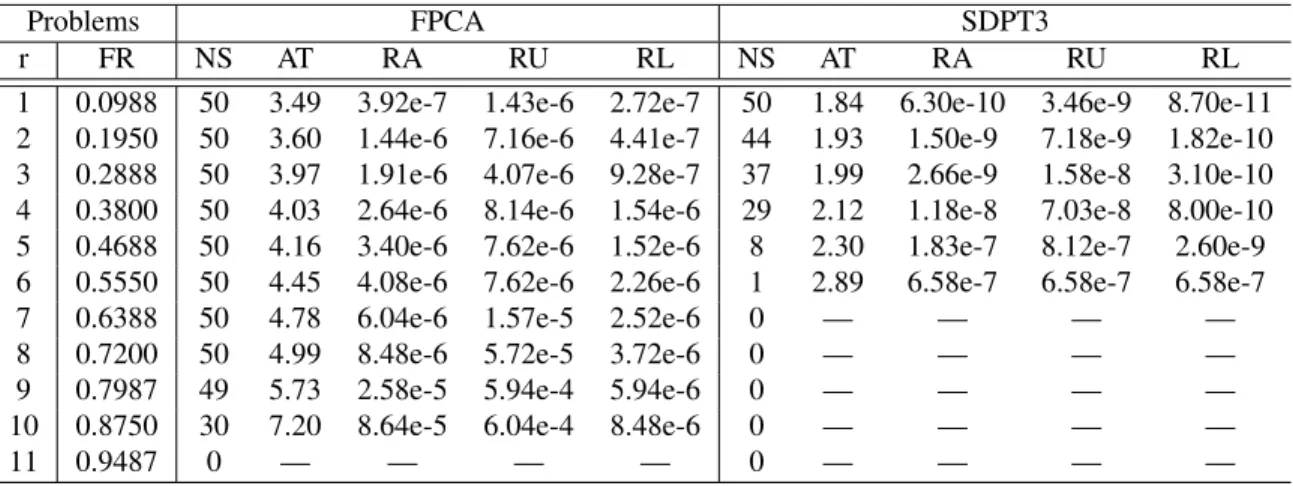
2.5 Numerical results for FPCA and SDPT3 for randomly created medium ma-trix completion problems (m=n=100) . . . 49
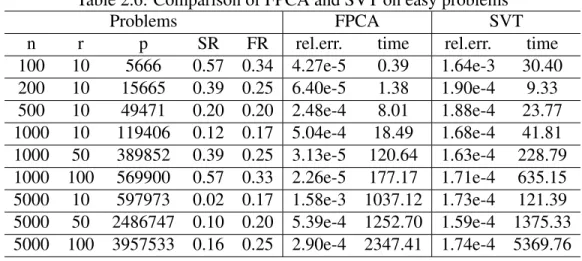
2.6 Comparison of FPCA and SVT on easy problems . . . 50
2.7 Comparison of FPCA and SVT on hard problems . . . 50
2.8 Numerical results for FPC1 for the Jester joke data set . . . 52
2.9 Numerical results for FPCA for the Jester joke data set (csis the number of rows we picked for the approximate SVD) . . . 52
2.10 Numerical results of FPCA for DNA microarray data sets . . . 55
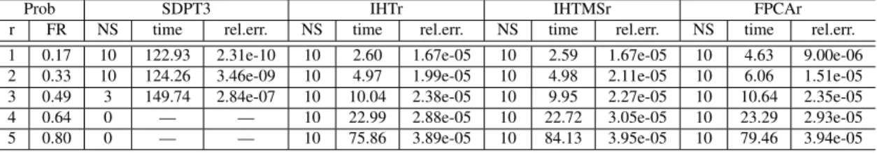
3.2 Comparison between IHTr, IHTMSr and FPCAr with SDPT3 . . . 85
3.3 Comparison between IHTr and IHT . . . 86
3.4 Comparison between IHTMSr and IHTMS . . . 87
3.5 Comparison between FPCAr and FPCA . . . 87
3.6 Comparison when the given rank is different from the true rank of 3 . . . . 88
3.7 Results on recovery of compressed video . . . 90
4.1 Comparison of the algorithms for solving (4.4.1) withρ=0.01 . . . 115
4.2 Comparison of the algorithms for solving (4.4.1) withρ=0.1 . . . 115
4.3 Comparison of ALM and EADM on surveillance video problems . . . 126
4.4 Numerical results for noisy matrix completion problems . . . 128
5.1 Comparison of MSA, FaMSA-v, Grad and Nest on solving Fermat-Weber problem (5.4.3) . . . 163
5.2 Comparison of MSA, FaMSA, FaMSA-s and Grad on solving TV-deblurring problem . . . 164
I feel very fortunate to have had the opportunity to work with my advisor, Donald Goldfarb. Don is an inspiring and creative mentor. His consistent support, encouragement and great sense of humor have made working with him a very joyful experience. Without his help, I could not have finished my dissertation.
I would like to express my sincere appreciation to the members of my dissertation committee, Garud Iyengar, Cliff Stein, Katya Scheinberg and Jonathan Eckstein, for their careful reading and valuable suggestions and comments on my dissertation. I learned a lot from the convex optimization, network flow and machine learning courses taught by Garud, Cliff and Katya. Their lectures really broadened my research scope. I would also like to thank Jonathan for many detailed and insightful comments to my papers and presentations. I am very grateful to my collaborators I have had the great opportunity to work with in the past five years. Specifically, I want to thank Amit Chakraborty and Wotao Yin for introducing me to the very exiting research area of medical imaging. The joint projects with Katya Scheinberg on machine learning significantly extended my research areas. I would also like to thank Zaiwen Wen, Lifeng Chen, Zhiwei Qin, Bo Huang, Necdet Serhat Aybat, Wei Liu and Jun Wang. The numerous fruitful discussions that we had have stimulated a lot of interesting and important joint papers. It was a privilege to have worked with such a group of talented people.
I would further like to thank people who have helped me during my career search. I especially want to thank Wotao Yin, Yinyu Ye, Yin Zhang, Garud Iyengar and Cliff Stein
faculty and stuff members for providing an enjoyable working environment.
I have made many very good friends during the past five years at Columbia University. I am very grateful to my friends Lifeng Chen, Zaiwen Wen, Zongjian Liu, Ning Cai, Xi-anhua Peng, Ming Hu, Thiam Hui Lee, Necdet Serhat Aybat, Yori Zwols, Yu Hang Kan, Guodong Pang, Min Wang, Yiping Du, Soonmin Ko, Ruxian Wang, Ranting Yao, Ana Zen-teno Langle, Yixi Shi, Pingkai Liu, Shuheng Zheng, Zhiwei Qin, Haowen Zhong, Xingbo Xu, Yina Lu, Xinyun Chen, Jing Dong, Juan Li, Zhen Qiu, Xin Li, Chen Chen, Yupeng Chen, Chun Wang, Yan Liu, Bo Huang, Ningyuan Chen, Yin Lu, for the fruitful discus-sions, for sharing ideas, and for every joyful and memorable moment we had. Especially, I owe my deepest gratitude to Jing, Haowen, Chun, Xingbo, Yina, Juan, Yupeng, Chen, Zhiwei, Lifeng, Ranting, Zongjian, for accompanying with me and taking very good care of me when I was once in need of helps in the Summer of 2010.
I am indebted to my parents Yinci Ma and Qiaoxia Wang. Their unconditional love and support throughout my life made it possible for me to come to the United States to pursue my career goal. My brother Shihao Ma provided happiness and joy to the family. I thank him for staying close to and taking care of my parents. I wish happiness will always be with my parents and my brother.
Shiqian Ma June 21, 2011
Chapter 1
Introduction
1.1
Background and Motivation
This dissertation is devoted to algorithms for solving problems with sparse or low-rank optimal solutions. Research in this area was mainly ignited by the recent emergence of compressed sensing (CS) and its matrix extensions such as the matrix completion and ro-bust principal component analysis (PCA) problems. CS enables one to recover a signal or image with fewer observations than the “length” of the signal or image, and thus pro-vides potential breakthroughs in applications where data acquisition is costly. For example, in magnetic resonance imaging (MRI) and computerized tomography (CT) problems, one tries to reduce the data acquisition time since patients suffer from keeping still or from exposure to ionizing radiation. However, the potential impact of CS cannot be realized without efficient optimization algorithms that can handle extremely large-scale and dense data from CS applications. Although the convex relaxations of these problems can be
re-formulated as either linear programming, second-order cone programming or semidefinite programming problems, the standard methods for solving these reformulations are not ap-plicable because the problems are usually of huge size and contain dense data. In this dissertation, we will give efficient algorithms for solving these “sparse” optimization prob-lems and analyze the convergence and iteration complexity properties of these algorithms.
1.2
Preliminaries
1.2.1
Basic Notation
We denote the set of real numbers byRand then-dimensional Euclidean space byRn. The superscript “⊤” denotes the transpose operation. The inner product of vectorsx∈Rnand
y∈Rn is denoted by⟨x,y⟩=x⊤y=∑nj=1xjyj. The Euclidean norm ofx∈Rn is denoted
by∥x∥2= (x⊤x)1/2. We use∥x∥0, the so-calledℓ0norm ofx∈Rn, to denote the number of nonzeros ofx. We use∥x∥1to denote theℓ1norm ofx, i.e.,∥x∥1=∑nj=1|xj|. ∥x∥∞denotes
the infinity norm, i.e., the largest component ofxin magnitude, i.e.,∥x∥∞=maxj|xj|.
We use Rm×n to denote the Euclidean space of the set of m×n matrices. rank(X) denotes the rank of the matrixX ∈Rm×n, i.e., the number of nonzero singular values ofX. If the rank of matrix X is r and its singular value decomposition (SVD) is given byX = ∑r
j=1ujσjv⊤j with singular valuesσ1≥σ2≥. . .≥σr >0, we denote by∥X∥∗ the nuclear
norm ofX, which is defined as the sum of singular values ofX, i.e., ∥X∥∗=∑rj=1σj. ∥X∥
i.e., ∥X∥=σ1. The Frobenius norm of X ∈Rm×n is defined as ∥X∥F = √
∑i,jXi j2. We
use vec(X) to denote the vector obtained by stacking the columns ofX ∈Rm×n as a long vector. We use∥X∥1and∥X∥∞to denote the norms corresponding to the vector form ofX, i.e.,∥X∥1:=∥vec(X)∥1and∥X∥∞:=∥vec(X)∥∞.
Diag(s)denotes the diagonal matrix whose diagonal elements are the elements of the vectors. sgn(t)is the signum function oft ∈R, i.e.,
sgn(t):= +1 ift >0, 0 ift =0, −1 ift <0,
while the signum multifunction oft∈Ris
SGN(t):=∂|t|= {+1} ift >0, [−1,1] ift =0, {−1} ift <0.
We use a⊙b to denote the elementwise multiplication of two vectors a and b. We use
X(k:l)to denote the submatrix ofX consisting of thek-th tol-th columns ofX.
Henceforth, we will write the linear map
A
(X) asA
X as this should not cause any confusion. For example,A
∗A
X:=A
∗(A
(X)).1.2.2
Sparse and Low-Rank Optimization
A fundamental problem in signal processing is to recover a sparse signal from a few mea-surements. This problem can be formulated as
min
x∈Rn ∥x∥0 s.t. Ax=b, (1.2.1)
wherexis the sparse signal one wants to recover,A∈Rm×nis the sensing matrix,b∈Rm
is the measurement and∥x∥0counts the number of nonzeros of x. Problem (1.2.1) can be interpreted as seeking the sparsest solution of a linear system. In some applications, the signal itself is not sparse but is sparse under some transformW ∈Rn×n. Then the problem can be formulated as
min
x∈Rn ∥W x∥0 s.t. Ax=b, (1.2.2)
i.e., the vector of coefficients ofx under transformW is expected to be sparse. Note that (1.2.2) can be reformulated in the form of (1.2.1) whenW is invertible
min
z ∥z∥0 s.t. AW
−1z=b.
It is known that (1.2.1) is usually NP-hard [73] and thus numerically intractable. Com-pressed sensing connects the NP-hard problem (1.2.1) to its convex relaxation, theℓ1
min-imization problem:
min
x∈Rn ∥x∥1 s.t. Ax=b, (1.2.3)
i.e.,∥x∥0 in the objective function is replaced by its convex envelope∥x∥1on the unit ball {x∈Rn|∥x∥∞≤ 1} (see, e.g., [54]). Compressed sensing theory guarantees that under certain conditions, the optimal solution of the NP-hard problem (1.2.1) is given by the optimal solution of the convex problem (1.2.3) with high probability (see [18, 26]). So now the question is how to solve the convex problem (1.2.3) efficiently. Although (1.2.3) can be reformulated as a linear programming problem and thus solved by interior point methods (IPMs), such methods are not practical since the problems arising from compressed sensing are usually of large scale. Sometimes the measurement bis contaminated by noise, then the constraintAx=bmust be relaxed, resulting in either the problem
min
x∈Rn ∥x∥1 s.t. ∥Ax−b∥2≤θ
or its Lagrangian version
min ρ∥x∥1+1
2∥Ax−b∥ 2
2, (1.2.4)
whereθ andρ are parameters. Many algorithms for solving the cardinality minimization problem (1.2.1) and theℓ1norm minimization problem (1.2.3) have been proposed. These include greedy algorithms [7, 8, 25, 27, 28, 74, 90, 94] for (1.2.1) and convex optimization
algorithms [17, 38, 50, 57, 101, 106] for (1.2.3) and its variant (1.2.4). See [24] for more information on the theory and algorithms for compressed sensing.
The matrix rank minimization problem is a matrix extension of theℓ0norm minimiza-tion problem (1.2.1). The matrix rank minimizaminimiza-tion problem can be written as
min
X∈Rm×n rank(X) s.t.
A
(X) =b, (1.2.5)where
A
:Rm×n→Rp is a linear map. This model has many applications such as deter-mining a low-order controller for a plant [42] and a minimum order linear system realiza-tion [36], and solving low-dimensional Euclidean embedding problems [65]. The matrix completion problemmin
X∈Rm×n rank(X) s.t. Xi j =Mi j, ∀(i,j)∈Ω, (1.2.6)
is a special case of (1.2.5), whereM∈Rm×nandΩis a subset of index pairs(i,j).The so called collaborative filtering problem [82, 87] can be cast as a matrix completion problem. Suppose users in an online survey provide ratings of some movies. This yields a matrixM
with users as rows and movies as columns whose(i,j)-th entryMi j is the rating given by
thei-th user to the j-th movie. Since most users rate only a small portion of the movies, we typically only know a small subset{Mi j|(i,j)∈Ω}of the entries. Based on the known
ratings of a user, we want to predict the user’s ratings of the movies that the user did not rate; i.e., we want to fill in the missing entries of the matrix. It is commonly believed that
only a few factors contribute to an individual’s tastes or preferences for movies. Thus the rating matrixMis likely to be ofnumericallow rank in the sense that relatively few of the top singular values account for most of the sum of all of the singular values. Finding such a low-rank matrixMcorresponds to solving the matrix completion problem (1.2.6).
The matrix rank minimization (1.2.5) is NP-hard in general due to the combinational nature of the function rank(·). Similar to the cardinality function ∥x∥0, we can replace rank(X) by its convex envelope to get a convex and more computationally tractable ap-proximation to (1.2.5). It turns out that the convex envelope of rank(X) on the set {X ∈
Rm×n:∥X∥ ≤1}is the nuclear norm∥X∥∗[35], i.e., the nuclear norm is the best convex
approximation of the rank function over the unit ball of matrices with spectral norm less than one. Using the nuclear norm as an approximation to rank(X) in (1.2.5) yields the nuclear norm minimization problem
min
X∈Rm×n∥X∥∗ s.t.
A
(X) =b. (1.2.7)As in the compressed sensing problem, ifbis contaminated by noise, the constraint
A
(X) =bmust be relaxed, resulting in either the problem
or its Lagrangian version
min ρ∥X∥∗+1
2∥
A
(X)−b∥ 22, (1.2.8)
whereθandρare parameters.
It was proved recently by Recht et al. [81] that under certain conditions, the optimal solution of (1.2.5) is given by the solution of (1.2.7). Thus, to solve the NP-hard problem (1.2.5), we only need to solve the convex problem (1.2.7).
For the matrix completion problem (1.2.6), the corresponding nuclear norm minimiza-tion problem is
min ∥X∥∗ s.t. Xi j =Mi j,(i,j)∈Ω. (1.2.9)
It was proved recently by Cand`es and Recht [16] and Cand`es and Tao [19] that, under certain conditions, (1.2.6) is equivalent to (1.2.9) in the sense that they have the same optimal solutions.
1.2.3
Iteration Complexity and Alternating Direction Methods
Chapters 4 and 5 focus on alternating direction type methods for solving the composite optimization problem min F(x)≡ K
∑
j=1 fj(x), (1.2.10)where fj,j=1,···,K are convex functions such that the following problems are easy to
solve for anyτ>0 andz∈Rnrelative to minimizingF(x):
min
x τfj(x) +
1
2∥x−z∥
2. (1.2.11)
In particular, we are specially interested in cases where solving (1.2.11) takes roughly the same effort as computing the gradient (or a subgradient) of fj(x). Problems of this type
arise in many applications of practical interest, including the followings that arise from sparse and low-rank optimization.
Example 1. ℓ1minimization in compressed sensing. The unconstrained compressed sensing problem
min 1
2∥Ax−b∥ 2
2+ρ∥x∥1,
is of the form of (1.2.10) with f(x) = 12∥Ax−b∥22 and g(x):=ρ∥x∥1. In this case, the
two problems (1.2.11) with fj= f and fj=gare easy to solve. Specifically, (1.2.11) with
fj = f reduces to solving a linear system and with fj =g reduces to a vector shrinkage
operation which requiresO(n)operations (see e.g., [50]).
Example 2. Nuclear norm minimization. The unconstrained nuclear norm mini-mization problem
min 1
2∥
A
(X)−b∥ 2is of the form of (1.2.10) with f(X) = 12∥
A
(X)−b∥22 and g(X) =ρ∥X∥∗. In this case, the problem (1.2.11) with fj = f reduces to solving a linear system. Problem (1.2.11)with fj =g has a closed-form solution that is given by matrix shrinkage operation (see
e.g., [68]).
Example 3. Robust principal component analysis (RPCA). The RPCA problem seeks to recover a low-rank matrixX from a corrupted matrixM. This problem has many applications in computer vision, image processing and web data ranking (see e.g., [15]), and can be formulated as
min
X,Y∈Rm×n ∥X∥∗+ρ∥Y∥1 s.t. X+Y =M, (1.2.12)
whereρ>0 andM∈Rm×n. Note that (1.2.12) can be rewritten as
min
X∈Rm×n ∥X∥∗+ρ∥M−X∥1,
which is of the form of (1.2.10). Moreover, the two problems (1.2.11) with fj=∥X∥∗and
fj =ρ∥M−X∥1 corresponding to (1.2.12) have closed-form solutions given respectively
by a matrix shrinkage operation and a vector shrinkage operation.
Example 4. Sparse inverse covariance selection (SICS). Gaussian graphical mod-els are of great interest in statistical learning. Because conditional independence between different nodes correspond to zero entries in the inverse covariance matrix of the Gaussian distribution, one can learn the structure of the graph by estimating a sparse inverse
covari-ance matrix from sample data by solving the following maximum likelihood problem with anℓ1-regularization term, (see e.g., [3, 39, 102, 107]).
max log det(X)− ⟨Σ,X⟩ −ρ∥X∥1,
or equivalently,
min −log det(X) +⟨Σ,X⟩+ρ∥X∥1, (1.2.13)
whereρ>0 andΣ∈S+n (the set of symmetric positive semidefinite matrices) is the sample covariance matrix. Note that by defining f(X):=−log det(X)+⟨Σ,X⟩andg(X):=ρ∥X∥1, (1.2.13) is of the form of (1.2.10). Moreover, it can be proved that the problem (1.2.11) with fj= f has a closed-form solution, which is given by a spectral decomposition, while
the solution of problem (1.2.11) with fj=gcorresponds to a vector shrinkage operation.
Example 5. Compressed sensing based MRI. One version of the compressed sensing magnetic resonance imaging (MRI) problem can be cast as minimizing the sum of three convex functions (see [69]):
min
x∈RnαTV(x) +β∥W x∥1+
1
2∥Ax−b∥
2, (1.2.14)
whereTV(x)is the total variation function,W is a wavelet transform, A∈Rm×n, b∈Rm
andα>0,β>0 are weighting parameters. The three problems (1.2.11) corresponding to (1.2.14) are also easy to solve.
For the composite convex optimization problems discussed above, since the problems (1.2.11) are easy to solve, alternating direction methods can be applied to solve them ef-ficiently. Despite of the efficiency of alternating direction methods, iteration complexity bounds for these methods were previously unknown. In Chapters 4 and 5 we propose several alternating direction type methods for solving the composite convex optimization problem (1.2.10). We prove that the iteration complexity of the basic version of these algorithms isO(1/ε)to obtain an ε-optimal solution. The iteration complexity of our ac-celerated algorithms is improved to O(1/√ε) for an ε-optimal solution, while the work required at each iteration is almost unchanged compared to the basic algorithms. To the best our knowledge, these iteration complexity results are the first ones of this type that have been given for alternating direction type methods.
Chapter 2
Fixed Point and Bregman Iterative
Methods for Matrix Rank Minimization
2.1
Introduction
Let us first consider the relationship between matrix rank minimization problem
min rank(X) s.t.
A
(X) =b, (2.1.1)and its convex relaxation, the nuclear norm minimization problem
and note that we can write the linear equations
A
(X) =bin (2.1.1) and (2.1.2) asA·vec(X) =b, (2.1.3)
where A∈Rp×mn is the matrix corresponding to the linear map
A
. An important ques-tion is: when will an optimal soluques-tion to the nuclear norm minimizaques-tion problem (2.1.2) give an optimal solution to matrix rank minimization problem (2.1.1). In response to this question, Recht et al. [81] proved that if the entries ofA are suitably random, e.g., i.i.d. Gaussian, then with very high probability, most m×n matrices of rank r can be recov-ered by solving the nuclear norm minimization (2.1.2) or equivalently, (2.1.3), wheneverp≥Cr(m+n)log(mn),whereCis a positive constant. For the matrix completion problem
min rank(X) s.t. Xi j =Mi j,(i,j)∈Ω, (2.1.4)
and its convex relaxation
min ∥X∥∗ s.t. Xi j =Mi j,(i,j)∈Ω, (2.1.5)
Theorem 2.1.1(Theorem 1.1 in [16]). Let M be an n1×n2matrix of rank r with SVD M= r
∑
k=1 σkukv⊤k,where the family {uk}1≤k≤r is selected uniformly at random among all families of r
or-thonormal vectors, and similarly for the family{vk}1≤k≤r. Let n=max(n1,n2). Suppose
we observe m entries of M with locations sampled uniformly at random. Then there are constants C and c such that if
m≥Cn5/4rlogn,
the minimizer to the problem(2.1.5)is unique and equal to M with probability at least1−
cn−3. In addition, if r≤n1/5, then the recovery is exact with probability at least1−cn−3 provided that
m≥Cn6/5rlogn.
This theorem states that a surprisingly small number of entries are sufficient to complete a low-rank matrix with high probability. Recently, this result was strengthened by Cand`es and Tao in [19], where it is proved that under certain incoherence conditions, the number of samples m that are required is only O(nrpolylog(n)). A similar result was shown by Keshavan et al. in [56].
The dual problem corresponding to the nuclear norm minimization problem (2.1.2) is
where
A
∗ is the adjoint operator ofA
. Both (2.1.2) and (2.1.6) can be rewritten as equiva-lent semidefinite programming (SDP) problems. The SDP formulation of (2.1.2) is:min X,W1,W2 1 2(Tr(W1) +Tr(W2)) s.t. W1 X X⊤ W2 ≽0
A
(X) =b, (2.1.7)where Tr(X)denotes the trace of the square matrixX. The SDP formulation of (2.1.6) is:
max z b ⊤z s.t. Im
A
∗(z)A
∗(z)⊤ In ≽0. (2.1.8)Thus to solve (2.1.2) and (2.1.6), we can use SDP solvers such as SeDuMi [89] and SDPT3 [100] to solve (2.1.7) and (2.1.8). Note that the number of variables in (2.1.7) is
1
2(m+n)(m+n+1). SDP solvers cannot usually solve a problem whenmandnare both much larger than 100.
Recently, Liu and Vandenberghe [67] proposed an interior-point method for another nuclear norm approximation problem
whereB∈Rm×nand
A
(x) =x1A1+x2A2+···+xpApis a linear mapping fromRptoRm×n.The equivalent SDP formulation of (2.1.9) is min x,W1,W2 1 2(Tr(W1) +Tr(W2)) s.t. W1 (
A
(x)−B)⊤A
(x)−B W2 ≽0. (2.1.10)Liu and Vandenberghe [67] proposed a customized method for computing the scaling di-rection in an interior point method for solving the SDP (2.1.10). The complexity of each iteration in their method was reduced fromO(p6)toO(p4)whenm=O(p)andn=O(p); thus they were able to solve problems up to dimensionm=n=350.
Another algorithm for solving (2.1.2) is due to Burer and Monteiro [12, 13], (see also Rennie and Srebro [82,87]). This algorithm uses the low-rank factorizationX=LR⊤of the matrixX ∈Rm×n, where L∈Rm×r,R∈Rn×r,r≤min{m,n},and solves the optimization problem min L,R 1 2(∥L∥ 2 F+∥R∥2F) s.t.
A
(LR⊤) =b. (2.1.11)It is known that as long as r is chosen to be sufficiently larger than the rank of the optimal solution matrix of the nuclear norm problem (2.1.2), this low-rank factorization problem is equivalent to the nuclear norm problem (2.1.2) (see e.g., [81]). The advantage
of this low-rank factorization formulation is that both the objective function and the con-straints are differentiable. Thus gradient-based optimization algorithms such as conjugate gradient algorithms and augmented Lagrangian algorithms can be used to solve this prob-lem. However, the constraints in this problem are nonconvex, so one can only be assured of obtaining a local minimizer. Also, how to chooseris still an open question.
One very interesting algorithm is the so called singular value thresholding algorithm (SVT) [14] which appeared almost simultaneously with our work. SVT is inspired by the linearized Bregman algorithms for compressed sensing and ℓ1-regularized problems. In [14] it is shown that SVT is efficient for large matrix completion problems. However, SVT only works well for very low rank matrix completion problems. For problems where the matrices are not of very low rank, SVT is slow and not robust and often fails.
Our algorithms have some similarity with the SVT algorithm in that they make use of
matrix shrinkage (see Section 2). However, other than that, they are very different. All of our methods are based on a fixed-point continuation (FPC) algorithm which uses an operator splitting technique for solving the unconstrained variant of (2.1.2),
minµ∥X∥∗+1
2∥
A
(X)−b∥ 22. (2.1.12)
By adopting a Monte Carlo approximate SVD in the FPC algorithm, we get an algorithm, which we call FPCA (Fixed-Point Continuation with Approximate SVD), that usually gets the optimal solution to (2.1.1) even if the condition of Theorem 2.1.1, or those for the affine constrained case, are violated. Moreover, our algorithm is much faster than
state-of-the-art SDP solvers such as SDPT3 applied to (2.1.7). Also, FPCA can recover matrices of moderate rank that cannot be recovered by SDPT3, SVT, etc. with the same number of samples. For example, FPCA can recover matrices of size 1000×1000 and rank 50 with a relative error of 10−5in about 3 minutes by sampling only 20 percent of the matrix elements. We know of no other method that has as good a recoverability property.
Outline. The rest of this chapter is organized as follows. In Section 2.2 we propose the fixed-point iterative algorithm for nuclear norm minimization problems. In Section 2.3 we analyze the convergence property of the fixed-point iterative algorithm. In Section 2.4 we discuss a continuation technique for accelerating the convergence of our algorithm. In Section 2.5 we propose a Bregman iterative algorithm for nuclear norm minimization extending the approach in [106] for compressed sensing to the rank minimization problem. In Section 2.6 we incorporate a Monte-Carlo approximate SVD procedure into our fixed-point continuation algorithm to speed it up and improve its ability to recover low-rank matrices. Numerical results for both synthesized matrices and real problems are given in Section 2.7. We give conclusions in Section 2.8.
2.2
Fixed-point iterative algorithm
Our fixed-point iterative algorithm for solving (2.1.12) is the following simple two-line algorithm: Yk=Xk−τg(Xk) Xk+1=Sτµ(Yk), (2.2.1)
whereSν(·)is the matrix shrinkage operator which will be defined later.
Our algorithm (2.2.1) is inspired by the fixed-point iterative algorithm proposed in [49] for theℓ1-regularized problem (1.2.4). The idea behind this algorithm is an operator split-ting technique. Note thatx∗is an optimal solution to (1.2.4) if and only if
0∈µSGN(x∗) +g∗, (2.2.2)
whereg∗=A⊤(Ax∗−b). For anyτ>0, (2.2.2) is equivalent to
0∈τµSGN(x∗) +τg(x∗). (2.2.3)
Note that the operatorT(·):=τµSGN(·) +τg(·)on the right hand side of (2.2.3) can be split into two parts: T(·) =T1(·)−T2(·),whereT1(·) =τµSGN(·) +I(·)andT2(·) =I(·)−τg(·).
Lettingy=T2(x∗) =x∗−τA⊤(Ax∗−b), (2.2.3) is equivalent to
Note that (2.2.4) is actually the optimality conditions for the following convex problem min x∗ τµ∥x ∗∥1+1 2∥x ∗−y∥2 2. (2.2.5)
This problem has a closed form optimal solution given by the so called vector shrinkage operator:
x∗=s˜ν(y),
whereν=τµ,and the vector shrinkage operator ˜sν(·)is given by ˜
sν(·) =sgn(·)⊙max{| · | −ν,0}. (2.2.6) Thus, the fixed-point iterative algorithm is given by
xk+1=s˜τµ(xk−τgk). (2.2.7)
Hale et al. [49] proved global and finite convergence of this algorithm to the optimal solution of theℓ1-regularized problem (1.2.4).
Motivated by this work, we develop a fixed-point iterative algorithm for (2.1.12). Since the objective function in (2.1.12) is convex, X∗ is the optimal solution to (2.1.12) if and
only if
0∈µ∂∥X∗∥∗+g(X∗), (2.2.8)
whereg(X∗) =
A
∗(A
(X∗)−b). Note that if the Singular Value Decomposition (SVD) ofX isX=UΣV⊤, whereU ∈Rm×r,Σ=Diag(σ)∈Rr×r,V ∈Rn×r,then (see e.g., [2, 9]) ∂∥X∥∗={UV⊤+W :U⊤W =0,WV =0,∥W∥2≤1}.
Hence, we get the following optimality conditions for (2.1.12):
Theorem 2.2.1. The matrix X ∈Rm×n with singular value decomposition X =UΣV⊤, U ∈Rm×r,Σ=Diag(σ)∈Rr×r,V ∈Rn×r,is optimal for the problem(2.1.12)if and only if there exists a matrix W ∈Rm×nsuch that
µ(UV⊤+W) +g(X) =0, (2.2.9a)
U⊤W =0,WV =0,∥W∥2≤1. (2.2.9b)
Now based on the optimality conditions (2.2.8), we can develop a fixed-point iterative scheme for solving (2.1.12) by adopting the operator splitting technique described at the beginning of this section. Note that (2.2.8) is equivalent to
for anyτ>0. If we let
Y∗=X∗−τg(X∗),
then (2.2.10) is reduced to
0∈τµ∂∥X∗∥∗+X∗−Y∗, (2.2.11)
i.e.,X∗is the optimal solution to
min X∈Rm×nτµ∥X∥∗+ 1 2∥X−Y ∗∥2 F (2.2.12)
In the following we will prove that the matrix shrinkage operator applied to Y∗ gives the optimal solution to (2.2.12). First, we need the following definitions.
Definition 2.2.2 (Nonnegative Vector Shrinkage Operator). Assume x∈Rn+. For any
ν>0, the nonnegative vector shrinkage operator sν(·)is defined as sν(x):=x,¯ withx¯i= xi−ν, if xi−ν>0 0, o.w.
Definition 2.2.3 (Matrix Shrinkage Operator). Assume X ∈Rm×n and the SVD of X is given by X =U Diag(σ)V⊤, U ∈Rm×r,σ∈Rr+,V ∈Rn×r. For any ν >0, the matrix
shrinkage operator Sν(·)is defined as
Sν(X):=U Diag(σ¯)V⊤, withσ¯ =sν(σ).
Theorem 2.2.4. Given a matrix Y ∈Rm×nwith rank(Y) =t, let its Singular Value Decom-position (SVD) be Y =UYDiag(γ)VY⊤, where UY ∈Rm×t,γ∈Rt+,VY ∈Rn×t. Then for any
scalarν>0,
X :=Sν(Y) =UYDiag(sν(γ))VY⊤ (2.2.13)
is an optimal solution of the problem
min X∈Rm×nf(X):=ν∥X∥∗+ 1 2∥X−Y∥ 2 F. (2.2.14)
Proof. Without loss of generality, we assumem≤n. Suppose that the solutionX ∈Rm×n
to problem (2.2.14) has the SVDX =UDiag(σ)V⊤,whereU ∈Rm×r,σ∈Rr+,V ∈Rn×r. Hence,X must satisfy the optimality conditions for (2.2.14) which are
0∈ν∂∥X∥∗+X−Y;
i.e., there exists a matrix
W =U¯ [ Diag(σ¯) 0 ] ¯ V⊤,
[V,V¯]are orthogonal matrices, such that 0=ν(UV⊤+W) +X−Y. (2.2.15) Hence, ˆ U νI+Diag(σ) 0 0 0 νDiag(σ¯) 0 Vˆ⊤−UYDiag(γ)VY⊤ =0. (2.2.16)
To verify that (2.2.13) satisfies (2.2.16), consider the following two cases:
Case 1: γ1 ≥γ2 ≥. . .≥γt >ν. In this case, choosing X as above, with r =t,U =
UY,V =VY andσ=sν(γ) =γ−νe, whereeis a vector ofrones, and choosing ¯σ=0 (i.e.,
W =0) satisfies (2.2.16).
Case 2: γ1≥γ2≥. . .≥γk>ν≥γk+1≥. . .≥γt.In this case, by choosingr=k,Uˆ(1 :
t) =UY,Vˆ(1 :t) =VY,σ=sν((γ1, . . . ,γk))and ¯σ1=γk+1/ν, . . . ,σ¯t−k=γt/ν,σ¯t−k+1=. . .= ¯
σm−r=0,X andW satisfy (2.2.16).
Note that in both cases, X can be written as the form in (2.2.13) based on the way we constructX.
Based on the above we obtain the fixed-point iterative scheme (2.2.1) stated at the beginning of this section for solving problem (2.1.12).
Moreover, from the discussion following Theorem 2.2.1 we have
Corollary 2.2.5. X∗is an optimal solution to problem(2.1.12)if and only if X∗=Sτµ(h(X∗)),
2.3
Convergence results
In this section, we analyze the convergence properties of the fixed-point iterative scheme (2.2.1). Before we prove the main convergence result, we need some lemmas.
Lemma 2.3.1. The shrinkage operator Sνis non-expansive, i.e., for any Y1and Y2∈Rm×n, ∥Sν(Y1)−Sν(Y2)∥F ≤ ∥Y1−Y2∥F. (2.3.1)
Moreover,
∥Y1−Y2∥F =∥Sν(Y1)−Sν(Y2)∥F ⇐⇒Y1−Y2=Sν(Y1)−Sν(Y2). (2.3.2)
Proof. Without loss of generality, we assume m ≤n. Assume SVDs of Y1 and Y2 are
Y1=U1ΣV1⊤andY2=U2ΓV2⊤, respectively, where
Σ= Diag(σ) 0 0 0 ∈Rm×n,Γ= Diag(γ) 0 0 0 ∈Rm×n,
σ= (σ1, . . . ,σs),σ1≥. . .≥σs>0 and γ= (γ1, . . . ,γt),γ1≥. . .≥γt >0. Note that here
U1,V1,U2andV2are (full) orthogonal matrices;Σ,Γ∈Rm×n. Suppose thatσ1≥. . .≥σk≥
ν>σk+1≥. . .≥σsandγ1≥. . .≥γl ≥ν>γl+1≥. . .≥γt, then
¯
where ¯ Σ= Diag(σ¯) 0 0 0 ∈Rm×n,Γ¯ = Diag(γ¯) 0 0 0 ∈Rm×n, ¯ σ= (σ1−ν, . . . ,σk−ν)and ¯γ= (γ1−ν, . . . ,γl−ν). Thus, ∥Y1−Y2∥2F− ∥Y¯1−Y¯2∥2F = Tr((Y1−Y2)⊤(Y1−Y2))−Tr((Y¯1−Y¯2)⊤(Y¯1−Y¯2)) = Tr(Y1⊤Y1−Y¯1⊤Y¯1+Y2⊤Y2−Y¯2⊤Y¯2)−2Tr(Y1⊤Y2−Y¯1⊤Y¯2) = s
∑
i=1 σ2 i − k∑
i=1 (σi−ν)2+ t∑
i=1 γ2 i − l∑
i=1 (γi−ν)2−2Tr(Y1⊤Y2−Y¯1⊤Y¯2). We note that Tr(Y1⊤Y2−Y¯1⊤Y¯2) = Tr((Y1−Y¯1)⊤(Y2−Y¯2) + (Y1−Y¯1)⊤Y¯2+Y¯1⊤(Y2−Y¯2)) = Tr(V1(Σ−Σ¯)⊤U1⊤U2(Γ−Γ¯)V2⊤+V1(Σ−Σ¯)⊤U1⊤U2Γ¯V2⊤+V1Σ¯⊤U1⊤U2(Γ−Γ¯)V2⊤ = Tr((Σ−Σ¯)⊤U(Γ−Γ¯)V⊤+ (Σ−Σ¯)⊤UΓ¯V⊤+Σ¯⊤U(Γ−Γ¯)V⊤),whereU =U1⊤U2,V =V1⊤V2are clearly orthogonal matrices. Now let us derive an upper bound for Tr(Y1⊤Y2−Y¯1⊤Y¯2). It is known that an orthogonal matrix U is a maximizing matrix for the problem
max{Tr(AU):U is orthogonal}
whenABis positive semidefinite, Tr(AB) =
∑
i σi(AB)≤∑
i σi(A)σi(B). (2.3.3)Thus, Tr((Σ−Σ¯)⊤U(Γ−Γ¯)V⊤), Tr((Σ−Σ¯)⊤UΓ¯V⊤)and Tr(Σ¯U(Γ−Γ¯)V⊤)achieve their maximum, if and only if (Σ−Σ¯)⊤U(Γ−Γ¯)V⊤, (Σ−Σ¯)⊤UΓ¯V⊤ and ¯ΣU(Γ−Γ¯)V⊤ are all positive semidefinite. Applying (2.3.3) to these three terms, we get Tr((Σ−Σ¯)⊤U(Γ−
¯
Γ)V⊤)≤∑iσi(Σ−Σ¯)σi(Γ−Γ¯), Tr((Σ−Σ¯)⊤UΓ¯V⊤)≤∑iσi(Σ−Σ¯)σi(Γ¯)and Tr(Σ¯U(Γ−
¯
Γ)V⊤)≤∑iσi(Σ¯)σi(Γ−Γ¯).Thus, without loss of generality, assumingk≤l ≤s≤t, we
have, ∥Y1−Y2∥2F− ∥Sν(Y1)−Sν(Y2)∥2F ≥
∑
s i=1 σ2 i − k∑
i=1 (σi−ν)2+ t∑
i=1 γ2 i − l∑
i=1 (γi−ν)2 −2(∑li=1σiν+∑si=l+1σiγi+∑ k i=1(γi−ν)ν+∑il=k+1σi(γi−ν)) = l∑
i=k+1 (2γiν−ν2+σ2i −2σiγi) + ( s∑
i=l+1 σ2 i + t∑
i=l+1 γ2 i − s∑
i=l+1 2σiγi). Now s∑
i=l+1 σ2 i + t∑
i=l+1 γ2 i − s∑
i=l+1 2σiγi≥0sincet≥sandσ2i +γ2i −2σiγi≥0. Also, since the function f(x):=2γix−x2is
monotoni-cally increasing in(−∞,γi]andσi<ν≤γi,i=k+1, . . . ,l,
Thus we get
D(Y1,Y2):=∥Y1−Y2∥2F− ∥Sν(Y1)−Sν(Y2)∥2F ≥0;
i.e., (2.3.1) holds.
Also, D(Y1,Y2) achieves its minimum value if and only if Tr((Σ−Σ¯)⊤U(Γ−Γ¯)V⊤), Tr((Σ−Σ¯)⊤UΓ¯V⊤)and Tr(Σ¯U(Γ−Γ¯)V⊤)achieve their maximum values simultaneously. Furthermore, if equality in (2.3.1) holds, i.e., D(Y1,Y2) achieves its minimum, and its minimum is zero, then k =l, s=t, and σi= γi,i=k+1, . . . ,s, which further implies
Σ−Σ¯ = Γ−Γ¯ and Tr((Σ−Σ¯)⊤U(Γ−Γ¯)V⊤) achieves its maximum. By applying the result 7.4.13 in [55], we get
Σ−Σ¯ =U(Γ−Γ¯)V⊤,
which further implies that
Y1−Y2=Sν(Y1)−Sν(Y2). (2.3.4) To conclude, clearly∥Sν(Y1)−Sν(Y2)∥F =∥Y1−Y2∥F if (2.3.4) holds.
The following two lemmas and theorem and their proofs are analogous to results and their proofs in Hale et al. [49].
Lemma 2.3.2. Let
A
X =Avec(X)and assume thatτ∈(0,2/λmax(A⊤A)). Then theoper-ator h(·) =I(·)−τg(·) is non-expansive, i.e., ∥h(X)−h(X′)∥F ≤ ∥X−X′∥F. Moreover,
Proof. First, we note that since τ∈(0,2/λmax(A⊤A)), −1<λi(I−τA⊤A)≤1,∀i,where
λi(I−τA⊤A)is thei-th eigenvalue ofI−τA⊤A. Hence,
∥h(X)−h(X′)∥F =∥(I−τA⊤A)(vec(X)−vec(X′))∥2≤ ∥I−τA⊤A∥2∥vec(X)−vec(X′)∥2
≤ ∥vec(X)−vec(X′)∥2=∥X−X′∥F.
Moreover,∥h(X)−h(X′)∥F =∥X−X′∥Fif and only if the inequalities above are equalities,
which happens if and only if
(I−τA⊤A)(vec(X)−vec(X′)) =vec(X)−vec(X′),
i.e., if and only ifh(X)−h(X′) =X−X′.
Lemma 2.3.3. Let X∗ be an optimal solution to problem(2.1.12), τ∈(0,2/λmax(A⊤A))
andν=τµ. Then X is also an optimal solution to problem(2.1.12)if and only if
∥Sν(h(X))−Sν(h(X∗))∥F ≡ ∥Sν(h(X))−X∗∥F =∥X−X∗∥F. (2.3.5)
Proof. The “only if” part is an immediate consequence of Corollary 2.2.5. For the “if” part, from Lemmas 2.3.1 and 2.3.2,
∥X−X∗∥F =∥Sν(h(X))−Sν(h(X∗))∥F ≤ ∥h(X)−h(X∗)∥F ≤ ∥X−X∗∥F.
Lemma 2.3.2 we obtain
Sν(h(X))−Sν(h(X∗)) =h(X)−h(X∗) =X−X∗,
which impliesSν(h(X)) =X sinceSν(h(X∗)) =X∗. It then follows from Corollary 2.2.5 thatX is an optimal solution to problem (2.1.12).
We now claim that the fixed-point iterations (2.2.1) converge to an optimal solution of problem (2.1.12). Similar convergence results for the problem of finding a zero of the sum of two maximal monotone operators can be found in [31, 40, 97].
Theorem 2.3.4. The sequence{Xk}generated by the fixed-point iterations with
τ∈(0,2/λmax(A⊤A))converges to some X∗∈
X
∗,whereX
∗is the set of optimal solutionsof problem(2.1.12).
Proof. Since bothSν(·)andh(·)are non-expansive,Sν(h(·))is also non-expansive. There-fore,{Xk}lies in a compact set and must have a limit point, say ¯X =limj→∞Xkj.Also, for
anyX∗∈
X
∗,∥Xk+1−X∗∥F =∥Sν(h(Xk))−Sν(h(X∗))∥F ≤ ∥h(Xk)−h(X∗)∥F ≤ ∥Xk−X∗∥F,
which means that the sequence{∥Xk−X∗∥F}is monotonically non-increasing. Therefore,
lim
k→∞∥X
k−X∗∥
where ¯X can be any limit point of{Xk}. By the continuity ofSν(h(·)), the image of ¯X, Sν(h(X¯)) = lim j→∞Sν(h(X kj)) = lim j→∞X kj+1,
is also a limit point of{Xk}. Therefore, we have
∥Sν(h(X¯))−Sν(h(X∗))∥F =∥Sν(h(X¯))−X∗∥F =∥X¯−X∗∥F,
which allows us to apply Lemma 2.3.3 to get that ¯X is an optimal solution to problem (2.1.12).
Finally, by settingX∗=X¯ ∈
X
∗in (2.3.6), we get thatlim k→∞∥X k−X¯∥ F = lim j→∞∥X kj−X¯∥ F =0,
i.e.,{Xk}converges to its unique limit point ¯X.
2.4
Fixed-point continuation
In this section, we discuss a continuation technique (i.e., homotopy approach) for acceler-ating the convergence of the fixed-point iterative algorithm (2.2.1).
2.4.1
Continuation
Inspired by the work of Hale et al. [49], we first describe a continuation technique to accelerate the convergence of the fixed-point iteration (2.2.1). Our fixed-point continuation (FPC) iterative scheme for solving (2.1.12) is outlined below. The parameterηµdetermines
the rate of reduction of the consecutiveµk, i.e.,
µk+1=max{µkηµ,µ¯}, k=1, . . . ,L−1
Algorithm 2.1Fixed-point Continuation (FPC)
Initialize: GivenX0, ¯µ>0. Selectµ1>µ2>···>µL =µ¯ >0.SetX =X0.
forµ=µ1,µ2, . . . ,µL do
whileNOT convergeddo
selectτ>0
computeY =X−τ
A
∗(A
(X)−b), and SVD ofY,Y =UDiag(σ)V⊤computeX =UDiag(sτµ(σ))V⊤
end while end for
2.4.2
Stopping criteria for inner iterations
Note that in the fixed-point continuation algorithm, in the k-th inner iteration we solve problem (2.1.12) for a fixedµ=µk. There are several ways to determine when to stop this
inner iteration, decreaseµand go to the next inner iteration. The optimality conditions for (2.1.12) is given by (2.2.9a) and (2.2.9b). Thus we can use the following condition as a stopping criterion:
wheregtol is a small positive parameter. However, the expense of computing the largest singular value of a large matrix greatly decreases the speed of the algorithm. Hence, we do not use this criterion as a stopping rule for large matrices. Instead, we use the criterion
∥Xk+1−Xk∥F
max{1,∥Xk∥
F}
<xtol, (2.4.2)
wherextol is a small positive number, since whenXk gets close to an optimal solutionX∗, the distance betweenXkandXk+1should become very small.
2.4.3
Debiasing
Debiasing is another technique that can improve the performance of FPC. Debiasing has been used in compressed sensing algorithms for solving (1.2.3) and its variants, where debiasing is performed after a support set
I
has been tentatively identified. Debiasing is the process of solving a least squares problem restricted to the support setI
, i.e., we solvemin ∥AIxI−b∥2, (2.4.3)
whereAI is a submatrix ofAwhose columns correspond to the support index set
I
, andxIis a subvector ofxcorresponding to
I
.Our debiasing procedure for the matrix completion problem differs from the procedure used in compressed sensing since the concept of a support set is not applicable. When we do debiasing, we fix the matricesUkandVkin the singular value decomposition ofXkand
then solve a least squares problem to determine the correct singular valuesσ∈Rr+; i.e., we solve
min
σ≥0 ∥
A
(UkDiag(σ)Vk⊤)−b∥2, (2.4.4)
wherer is the rank of current matrix Xk. Because debiasing can be costly, we use a rule proposed in [104] to decide when to do it. In the continuation framework, we know that in each subproblem with a fixedµ,∥Xk+1−Xk∥F converges to zero, and∥g∥2converges toµ
whenXk converges to the optimal solution of the subproblem. We therefore choose to do
debiasing when∥g∥2/∥Xk+1−Xk∥F becomes large because this indicates that the change
between two consecutive iterates is relatively small. Specifically, we call for debiasing in the solver FPC3 (see Section 2.7) when∥g∥2/∥Xk+1−Xk∥F >10.
2.5
Bregman iterative algorithm
Algorithm FPC is designed to solve (2.1.12), an optimal solution of which approaches an optimal solution of the nuclear norm minimization problem (2.1.2) asµ goes to zero. However, by incorporating FPC into a Bregman iterative technique, we can solve (2.1.2) by solving a limited number of instances of (2.1.12), each corresponding to a differentb.
Given a convex functionJ(·), the Bregman distance [11] of the pointufrom the pointv
is defined as
where p∈∂J(v)is some subgradient in the subdifferential ofJ at the pointv.
Bregman iterative regularization was introduced by Osher et al. in the context of image processing [79]. Specifically, in [79], the Rudin-Osher-Fatemi [83] model
u=argminu µ ∫ |∇u|+1 2∥u−b∥ 2 2 (2.5.2)
was extended to an iterative regularization model by replacing the total variation functional
J(u) =µTV(u) =µ
∫
|∇u|,
by the Bregman distance with respect toJ(u). This Bregman iterative regularization pro-cedure recursively solves
uk+1←min u D pk J (u,u k ) +1 2∥u−b∥ 2 2 (2.5.3)
for k=0,1, . . . starting withu0 =0 and p0=0. Since (2.5.3) is a convex programming problem, the optimality conditions are given by0∈∂J(uk+1)−pk+uk+1−b,from which we get the update formula forpk+1:
Therefore, the Bregman iterative scheme is given by uk+1←minuDp k J (u,uk) + 1 2∥u−b∥ 2 2 pk+1=pk+b−uk+1. (2.5.5)
Interestingly, this turns out to be equivalent to the iterative process
bk+1=b+ (bk−uk) uk+1←minuJ(u) + 1 2∥u−b k+1∥2 2, (2.5.6)
which can be easily implemented using existing algorithms for (2.5.2) with different inputs
b. Interestingly, Bregman methods (2.5.5) and (2.5.6) were later found to be equivalent to the classical augmented Lagrangian method (see, e.g., [106]).
Subsequently, Yin et al. [106] proposed solving the basis pursuit problem (1.2.3) by applying the Bregman iterative regularization algorithm to
min x J(x) + 1 2∥Ax−b∥ 2 2
forJ(x) =µ∥x∥1,and obtained the following two equivalent iterative schemes analogous to (2.5.5) and (2.5.6), respectively:
• Version 1:
– x0←0,p0←0, – fork=0,1, . . .do
– xk+1←argminxDJpk(x,xk) +1 2∥Ax−b∥ 2 2 – pk+1←pk−A⊤(Axk+1−b) • Version 2: – b0←0,x0←0, – fork=0,1, . . .do – bk+1←b+ (bk−Axk) – xk+1←argminxJ(x) +1 2∥Ax−b k+1∥2 2.
One can also use the Bregman iterative regularization algorithm applied to the uncon-strained problem (2.1.12) to solve the nuclear norm minimization problem (2.1.2). That is, one iteratively solves (2.1.12) by
Xk+1←min X D pk J (X,X k ) +1 2∥
A
(X)−b∥ 2 2, (2.5.7)and updates the subgradient pk+1by
pk+1:= pk−
A
∗(A
(Xk+1)−b), (2.5.8)Equivalently, one can also use the following iterative scheme: bk+1←b+ (bk−
A
(Xk)) Xk+1←arg minXµ∥X∥∗+ 1 2∥A
(X)−b k+1∥2 2. (2.5.9)Thus, our Bregman iterative algorithm for nuclear norm minimization (2.1.2) can be outlined as follows. The last step can be solved by Algorithm FPC.
Algorithm 2.2Bregman Iterative Algorithm
b0←0,X0←0, fork=0,1, . . .do bk+1←b+ (bk−
A
(Xk)), Xk+1←arg minXµ∥X∥∗+ 1 2∥A
(X)−b k+1∥2 2. end for2.6
An approximate SVD based FPC algorithm: FPCA
Computing singular value decompositions is the main computational cost in Algorithm FPC. Consequently, instead of computing the full SVD of the matrixY in each iteration, we implemented a variant of algorithm FPC in which we compute only a rank-ks
approx-imation toY, where ks is a heuristically determined parameter. We call this approximate
SVD based FPC algorithm (FPCA). This approach greatly reduces the computational ef-fort required by the algorithm. Specifically, we compute an approximate SVD by a fast Monte Carlo algorithm: the Linear Time SVD algorithm developed by Drineas et al. [30]. For a given matrixA∈Rm×n, and parameterscs,ks∈Z+with 1≤ks≤cs≤nand{pi}ni=1,