ISSN: 2502-4752, DOI: 10.11591/ijeecs.v11.i3.pp1162-1167 1162
Identification of Rainfall Patterns on Hydrological Simulation
Using Robust Principal Component Analysis
S.M. Shaharudin1, N. Ahmad2, N.H. Zainuddin3, N.S. Mohamed4 1,3Department of Mathematics, Faculty of Science and Mathematics, Universiti Pendidikan Sultan Idris, Malaysia 2
Department of Mathematics, Faculty of Science, Universiti Teknologi Malaysia, Malaysia 4
Technical Foundation, Malaysian Institute of Industrial Technology, Universiti Kuala Lumpur, Malaysia
Article Info ABSTRACT
Article history: Received Apr 8, 2018 Revised Jun 9, 2018 Accepted Jun 23, 2018
A robust dimension reduction method in Principal Component Analysis (PCA) was used to rectify the issue of unbalanced clusters in rainfall patterns due to the skewed nature of rainfall data. A robust measure in PCA using Tukey’s biweight correlation to downweigh observations was introduced and the optimum breakdown point to extract the number of components in PCA using this approach is proposed. A set of simulated data matrix that mimicked the real data set was used to determine an appropriate breakdown point for robust PCA and compare the performance of the both approaches. The simulated data indicated a breakdown point of 70% cumulative percentage of variance gave a good balance in extracting the number of components. The results showed a more significant and substantial improvement with the robust PCA than the PCA based Pearson correlation in terms of the average number of clusters obtained and its cluster quality. Keywords:
Breakdown point Cluster analysis
Principal component analysis Simulation
Tukey’s biweight correlation
Copyright © 2018 Institute of Advanced Engineering and Science. All rights reserved.
Corresponding Author: S.M. Shaharudin,
Department of Mathematics, Faculty of Science and Mathematics, Universiti Pendidikan Sultan Idris,
35900 Tanjung Malim, Perak, Malaysia. Email: [email protected]
1. INTRODUCTION
The identification of spatial torrential rainfall pattern is an essential task for hydrologist or climatologist to classify hydrologic events in order to simplify hydrologic convolution. For such purposes, measurements of rainfall amount for time series records observed at several rain gauge stations had a long record of data are examined. Thus, identifying rainfall patterns can be difficult in such high dimensional data set as it may contain high degree of irrelevant and redundant information which may significantly degrade the performance of further analysis.
Clustering techniques preceded by principal component analysis (PCA) are often combined to identify key spatial patterns in the data by reducing the number of variables for clustering cases [1]-[3]. A typical approach in PCA requires the use of configuration points of entities between the rows and column of the data based on Pearson correlation matrix. Pearson correlation is commonly used in the derivation of T-mode correlation to measure similarity between the daily rainfall especially in countries that experience four seasons [4]-[6]. Pearson correlation matrix is calculated by finding the covariance of variables and dividing it by the square root of the product of the variances. However, a PCA based Pearson correlation matrix may not be suitable for all types of rainfall data, particularly in the tropical region. More precisely, the data are inherently skewed, usually to the right, as such data only take positive values and tend to be skewed towards higher values. In severely skewed distributions, Pearson correlation gradually loses its advantages especially for high dimensional data or large correlation matrix [7].Thus, applying PCA based
Pearson correlation on rainfall data especially in Peninsular Malaysia could affect cluster partitions and generate extremely unbalanced clusters in a high dimensional space.
To overcome the issues above, Tukey's biweight correlation matrix is introduced for the analysis of spatial distribution torrential rainfall patterns, as an alternative of the Pearson correlation matrix. PCA based Tukey’s biweight correlation shows differentiating patterns on the number of clusters produced at different cumulative percentage of variation used. In climatology studies particularly in identifying rainfall patterns, it is more reasonable to obtain more than two cluster partitions to explain the various types of rainfall patterns.
Tukey's biweight correlation is based on Tukey's biweight function that relies on M-estimators used in robust correlation estimates. This approach is more resistant for outlying values as it examines each observation and down-weights those that lie far from the center of the data. Another important part in Tukey’s biweight correlation is a breakdown point. According to the study, the breakdown point is used in measuring their resistance in outlying data values [8]. However, in PCA based Tukey’s biweight correlation, the breakdown point is used to determine the best number of components to extract.
In order to assess the performance of the PCA based Tukey’s biweight correlation, we illustrate the proposed and classical method on several sets of simulated data matrices that mimic the real data. These simulated data matrices follow the distribution of the original torrential rainfall data in Peninsular Malaysia. The purpose of using simulation is to determine an appropriate breakdown 9 point and to evaluate the performance of the both methods in the analysis of identifying spatial cluster torrential rainfall patterns in Peninsular Malaysia.
2. RESEARCH METHOD
In this study, the focus is on the occurrence of extreme rainfall event described as torrential rainfall. It was therefore necessary to choose some criteria that would lead to the establishment of a threshold, in order to allow for a clear distinction between what constitutes a day of torrential rainfall in the Peninsular Malaysia region and what does not. The range of threshold for torrential rainfall data in Peninsular Malaysia is 60 mm/day. This threshold is chosen based on the categorization of rainfall intensity by Jabatan Pengairan dan Saliran (JPS). By filtering days with rainfall more than 60 mm for at least 2% of overall stations, 250 days and 15 rainfall stations were obtained which in turn were suffice enough to represent the main torrential centers.
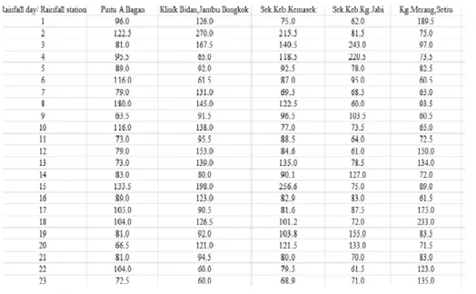
Figure 1 shows the matrix of daily torrential rainfall data after filtering from raw data based on the threshold that set to the data. The rainfall day in the first column refers to the rainfall observation and the rainfall station in the first row refers to the variable. Rainfall is often expressed in millimeters per day (mm/day) which represents the total depth of rainwater (mm), in 24 hours. From Figure 2 and Table 1, it appeared that the locations where these torrential rainfall occur and were largely located at two regions specifically the Northern and Eastern region.
Figure 1. An example of a snapshot of the daily torrential rainfall data consisting of daily amount of rainfall data recorded at several locations
Figure 2. Rainfall stations that represent the main torrential centers in Peninsular Malaysia
Table 1. List of the Rainfall Stations According the Monsoon Occurred
Region Station Code
Northeast PintuA.Bagan,AirItam N1
Selama N2
KlinikBkt. Bendera N3
East KlinikBidan ,JambuBongkok E7
Sek. Keb. Kemasek E5
Sek. Keb. Kg. Jabi E11
Kg. Merang ,Setiu E10
Endau E1
Rumah Pam Pahang Tua,Pekan E2
Kuantan E3
JPS Kemaman E4
Sek.Men. Sultan Omar, Dungun E6
Kg. Menerong E8
Stor JPS Kuala Trengganu E9
Kota Bharu E12
3. METHODOLOGY
3.1. Principal Component Analysis based Pearson Correlation
PCA is designed to reduce the number of variables of interest into a smaller set of components while retaining most of the significant information [9], [10]. This is achieved by converting a set of observations of possibly correlated variables into a set of linearly uncorrelated variables called principal components. The first principal component accounts for as much of the variation in the original data. Then each succeeding component accounts for as much of the remaining variation subject to being uncorrelated with the previous component.
Covariance or correlation matrix derived from the data matrix plays an important role in PCA to calculate its eigenvalues and eigenvectors to obtain the associated components that account for most of the variations in the data [11]. For the purpose of this study, correlation matrix is used. It is generally recommended taking at least 70% of cumulative percentage of total variation as a benchmark to cut off the eigenvalues in a large data set for extracting the number of components [12]. The reduced matrix is the component matrix of eigenvector ―loadings‖ which defines the new variables consisting of linear transformation of the original variables that maximizes the variance in the new axes.
The steps involved in PCA algorithm are as follows: Step 1 : Obtain the input matrix.
Step 2 : Calculate its correlation matrix.
Step 3 : Calculate the eigenvectors and eigenvalues of the correlation matrix.
Step 4 : Select the most important principal components based on cumulative percentage of total variation. Step 5 : Derive the new data set
Step 6 : Calculate Calinski and Harabasz index in new data set to determine the best number of cluster Step 7 : Apply k-means method to new data set
3.2. Principal Component Analysis based Tukey’s Biweight Correlation
PCA based Tukey’s biweight correlation is proposed to overcome the problem that address in Section 1. Before proceeding, the original data matrix is standardized by a robust location and scale estimator to avoid any masking or swamping effect [13]. The reduced data set is then applied to K-Means cluster analysis to obtain cluster partitions. K means method requires specifying the number of clusters before the algorithm is applied. To overcome this problem, Calinski and Harabasz Index [14] is used as a measure to determine the optimal number of cluster partition for the input data. This is indicated by the maximum value of the index.
The steps involved in the proposed algorithm are as follows [15]: Step 1 : Obtain the input matrix.
Step 2 : Standardize the observation with median and mean absolute deviation (MAD), i.e.
̅
(| ( )|)
such that refer to elements in the input matrix.
Step 3 : Set the breakdown point for the Tukey's biweight correlation at 0.4 Step 4 : Calculate the Tukey's biweight correlation matrix.
Step 5 : Calculate the eigenvectors and eigenvalues of the correlation matrix.
Step 6 : Select the most important principal components based on cumulative percentage of total variation. Step 7 : Derive the new data set
Step 8 : Calculate Calinski and Harabasz index in new data set to determine the best number of cluster Step 9 : Apply k-means method to new data set
3.3. Data model of rainfall for the simulation procedure
Data sets are generated based on probability distributions that mimic a multivariate torrential rainfall data. The distributions of tropical rainfall data are generally skewed to the right and thus distributions that exhibit this characteristic can be used to model the torrential rainfall. Three distributions are chosen which are gamma, Log-Normal and Generalized Pareto distribution (GPD) are tested on multivariate rainfall data. These distributions are commonly used as potential candidates for the data generating mechanism of rainfall data [16], [17]. Estimation of the parameters for each of the above sampled probability distributions are based on the summary statistics from the original torrential rainfall data in Peninsular Malaysia. These parameters are based on the mean and standard deviation from the data set of 250 torrential rainfall days and 15 rainfall stations of the original torrential rainfall data for the 33 year period in Peninsular as described in Section 2. The shape parameter for this study is ξ=0.2 where it performs well for and very good for [18].
Out of the three probability distributions which were sampled, GPD appears to fit the data set based on several assessments by distribution graphs (i.e QQ plot and probability different graph) and goodness of fit tests using Chi-square and Anderson Darling test. This distribution is remarkably good at significance level if , thus providing some evidence that the null hypothesis is true (i.e the GPD provides the correct statistical model for rainfall data).
Simulations were carried out on sample GPD distributions characterized by three parameters location μ=104.8, scale σ=54.7 and shape ξ=0.2, obtained from the original torrential rainfall data of 33 year period in Peninsular Malaysia to construct an n x p matrix with and to represent 250 torrential rainfall days and 15 rainfall stations respectively as described in Section 2. In order to vary the simulation tested, two different settings are used. Firstly, the scale (i.e. standard deviation) are varied below and above standard deviation of the original torrential rainfall data to assess the effect of preserving most of the variations in the data. All generated data clearly contains values of around 60 which reflect the 60mm/day threshold of torrential rainfall. Secondly, several range of breakdown points between 0.2 to 0.8 are tested to evaluate the influence selection of the significance number of components to extract in PCA.
Each set of generated data are then employed to the two approaches, PCA based Pearson correlation and robust PCA based Tukey’s biweight correlation as described in Section 3.1 and Section 3.2. From these two approaches, their findings will be compared according to cluster partition and generate extremely unbalanced clusters rainfall patterns. In addition for robust PCA based Tukey’s biweight correlation, the choice of appropriate breakdown point is discussed due to determine in extracting number of component in PCA.
4. RESULTS AND DISCUSSION
The performance of robust PCA based on Tukeys’ biweight correlation are compared against PCA approaches using the simulated data described in Section 3. Table 2 shows the average number of components obtained using robust PCA based Tukey’s biweight correlation from 20 simulated data. It visualizes that the choice of breakdown point would influence the extracting number of components in this approach. From Table 2, a higher breakdown point (r=0.8) will lead to flagging fewer significance components to extract. A breakdown points of r=0.4 gives a good balance in extracting number of components where it retains sufficient components where only 12 components have been retained. In hydrological data, extracting too many components is not favorable as it may reflect variations of low frequency or spatial scale that are not important [19]. Hence, the choice of breakdown point is very important in PCA based Tukey’s biweight correlation.
The entries in Table 3 show the average number of components and clusters obtained from PCA based Pearson correlation and PCA based Tukey’s biweight correlation at an increasing cumulative percentage of variation from 60% to 80%. Each of these average numbers of components and clusters (round up to two decimal places) are obtained from the 20 simulated data as explained in Section 3. Note that the variation between the simulated data at each level of cumulative percentage of variations, components and clusters is small (0.44 to 0.94).
Table 2. The Average Number of Components Based on 70% Cumulative Percentage of Variance in Several Values of Breakdown Point
Breakdown Point, Number of Components
0.2 9
0.4 12
0.6 6
0.8 3
Table 3. Average Number of Components and Clusters Obtained based on Pearson and Tukey’s Biweight Correlation from 20 Simulated Data
Cum.%
Number of components
Number of cluster, K
Tukey's biweight Pearson Tukey's biweight Pearson
Mean Std.Dev. Mean Std.Dev. Mean Std.Dev. Mean Std.Dev.
60 2.25 0.44 45.40 0.82 9.50 0.69 2.40 0.60
65 5.55 0.76 54.05 0.89 5.10 0.85 2.40 0.50
70 11.55 0.94 61.50 0.83 8.40 0.88 2.35 0.49
75 19.80 0.89 71.55 0.89 11.50 0.94 2.25 0.55
80 28.75 0.92 82.50 0.69 2.40 0.50 2.35 0.59
It is observed from Table 3 that there is a difference in the average number of components and the number of clusters obtained from these two correlation measures in PCA at each level of cumulative percentage of variations. It appears that PCA based Tukey's biweight correlation requires less number of components to extract in order to achieve at least 70% of cumulative percentage of variation compared to PCA based Pearson correlation. For instance, 28.75 ≈ 29 components are retained with robust PCA based Tukey’s as compared to 82.50 ≈ 83 with PCA based Pearson’s at 80% cumulative percentage of variation. Inclusion of too many principal components inflates the importance of outlier, thus the results become poorly in identifying rainfall patterns.
In terms of cluster partitions, Table 3 also shows that in contrast to PCA based Pearson’s, PCA based Tukey's biweight correlation is more sensitive to the number of clusters according to the number of components retained. The number of clusters as a result of PCA based Pearson correlation, appear to stabilize at only two clusters regardless of the cumulative percentage of variation used. In hydrological studies particularly in identifying rainfall patterns, it is more reasonable to obtain more than two cluster partitions to explain the various types of rainfall patterns. Thus, two clusters clearly is inappropriate as it masks the true structure of the data.
In order to examine the cluster solutions, the clustering output at 70% cumulative percentage of variation on PCA based Tukey’s biweight correlation (8.40 ≈ 8 clusters) and PCA based Pearson correlation (2.35 ≈2 clusters) are chosen respectively. Therefore, from the results that we discuss above, it can be concluded that PCA based Tukey’s biweight correlation prove that it is an efficient robust method when dealing with hydrological data especially in rainfall data where it shows a substantial improvement in the
cluster partition with PCA based Tukey’s biweight correlation than PCA based Pearson’s to avoid inaccurate unbalanced clusters in rainfall data
5. CONCLUSION
The robust PCA based Tukey’s biweight correlation has been shown as a promising contender to the existing PCA based Pearson correlation. Specifically, robust PCA based Tukey’s biweight correlation showed a substantial improvement in the cluster partition as compared to PCA based Pearson correlation and it has been proven by the simulation results. The simulated data indicates a breakdown point of 70% cumulative percentage of variance to give a good balance in extracting the number of components to avoid variations of low frequency or insignificant spatial scale in the clusters.
REFERENCES
[1] Moron V, Robertson AW, Qian JH, Ghil M. Weather Types Across the Maritime Continent: from the Diurnal Cycle to Interannual Variations. Frontiers in Environmental Science. 2015; 3(44): 1-19.
[2] Ahmad NH, Othman IR, Deni SM. Hierarchical Cluster Approach for Regionalization of Peninsular Malaysia based on the Precipitation Amount. Journal of Physics: Conference Series. 423. 2013; 1-10.
[3] Siva GS, Rao VS, Babu DR. Cluster Analysis Approach to Study the Rainfall Pattern in Visakhapatnam District.
Weekly Science Research Journal. 2014;1(31).
[4] Shaharudin SM, Ahmad N, Yusof F, Yap XQ. The Comparison of T-mode and Pearson Correlation Matrices in Classification of Daily Rainfall Patterns in Peninsular Malaysia. Matematika. 2013; 29(1c), 187-194.
[5] Amiri MA, Mesgari MS. Modeling the Spatial and Temporal Variability of Precipitation in Northwest Iran. Atmosphere. 2017; 8(254), 1-14.
[6] Neeti N. Extending T-Mode Canonical Correlation Analysis to T-Mode Pre-Filtered Canonical Correlation Analysis: A Novel Approach To Discover Shared Patterns Between Two Image Time Series. International Journal of Remote Sensing. 2014, 35(4), 1926-1935.
[7] Raymaekers, J, Rousseeuw PJ. Fast Robust Correlation for High Dimensional Data. Dept. of Mathematics, KU Leuven, Belgium. arXiv:1712.05151. 2018.
[8] Owen M.Tukey's Biweight Correlation and the Breakdown. Master Thesis. California: Pomona College; 2010. [9] Sahak R, Mansor W, Lee KY, Zabidi A. Performance of Principal Component Analysis and Orthogonal Least
Square on optimized Feature Set in Classifying Asphyxiated Infant Cry using Support Vector Machine. Indonesian Journal of Electrical Engineering and Computer Science. 2018; 9(1), 139-145.
[10] Ruilian W, Shengjian G. Comprehensive Evaluation to Distribution Network Planning Schemes using Principal Component Analysis Method. TELKOMNIKA Indonesian Journal of Electrical Engineering. 2014; 12(8), 5897-5904.
[11] Neware S, Mehta K, Zadgaonkar AS. Finger Knuckle Identification using Principal Component Analysis and Nearest Mean Classifier. International Journal of Computer Applications. 2013; 70(9): 18-23.
[12] Shaharudin SM, Ahmad N. Modeling, Design and Simulation Systems. In: Ali MSM, Sahlan S, Wahid H, Yunus MAM, Subha NAM and Wahap AR. 752. Singapore: Springer; 2017: 216-224.
[13] Choulakian V. Robust Q-Mode Principal Component Analysis in L1. Computational Statistics & Data Analysis. 2001; 37: 135-150.
[14] Maulik U. 2002. Performance Evaluation of SomeClustering Algorithms and Validity Indices. IEEE Transactions of Pattern Analysis and Machine Intelligence. 2002; 24(12): 1650-1654.
[15] Shaharudin SM, Ahmad N, Yusof F. Improved Cluster Partition in Principal Component Analysis Guided Clustering. International Journal of Computer Applications. 2013; 75(11): 22-25.
[16] Cho H-K, Bowman K.P, North G.R. A Comparison of Gamma and Lognormal Distribution for Characterizing Satellite Rain Rates from the Tropical Rainfall Measuring Mission. Journal of Applied Meteorology. 2004; 43: 1586-1597.
[17] Dhore K.A, Nathan KK, Khare D, Chaube U.C. Weekly Rainfall Prediction using the Standard Package SMADA. Proceedings of the International Conference on Water and Environment (WE-2003). 15-18 December 2003. Bhopal. 2003: 32-39.
[18] De Zea Bermudez P, Kotz S. Parameter Estimation of the Generalized Pareto Distribution—Part I. Journal of Statistical Planning and Inference. 2010; 140(6), 1353-1373.
[19] Mimmack GM, Mason SJ, Galpin JS. Choice of Distance Matrices in Cluster Analysis : Defining Regions. Journal of Climate. 2002; 14: 2790-2797.