Feature Selection with Attributes Clustering by Maximal Information Coefficient

(1)

Procedia Computer Science 17 ( 2013 ) 70 – 79

Selection and peer-review under responsibility of the organizers of the 2013 International Conference on Information Technology and Quantitative Management

doi: 10.1016/j.procs.2013.05.011

Information Technology and Quantitative Management , ITQM 2013

Feature Selection with Attributes Clustering by Maximal

Information Coe

ﬃ

cient

Selection and peer-review under responsibility of the organizers of the 2013 International Conference on Information Technology and Quantitative Management

Xi Zhao

a,b

, Wei Deng

c

, Yong Shi

a,b,c,∗ a_{University of Chinese Academy of Sciences, Beijing, China}

b_{Research Center on Fictitious Economy}_&_{Data Science of Chinese Academy of Sciences, Beijing, China} c_{College of Information Science and Technology University of Nebraska at Omaha, Omaha, NE, 68182, USA}

Abstract

Feature selection is usually a separate procedure which can not benefit from result of the data exploration. In this paper, we propose a unsupervised feature selection method which could reuse a specific data exploration result. Furthermore, our algorithm follows the idea of clustering attributes and combines two state-of-the-art data analyzing methods, that’s maximal information coefficient and affinity propagation. Classification problems with different classifiers were tested to validation our method and others. Data experiments result exhibits our unsupervised algorithm is comparable with classical feature selection methods and even outperforms some supervised learning algorithms. Data simulation with one credit dataset of our own from a bank of China shows the capability of our method for real world application.

Keywords: feature selection, feature clustering, maximal information coeﬃcient, aﬃnity propagation

1. Introduction

Data mining shows powerful capability for automatically identifying valuable and potential information from data, so lots of area have been profit from it, such as expert system, decision support and financial forecast[1]. Due to the widespread use of the Internet and the emergence of bioinformatics, the dimensionality of dataset become larger and larger. Datasets with hundreds and thousands of attributes may cause the “curse of dimensionality” problem. Furthermore, some of traditional classification and clustering algorithms can not work properly. One of the most feasible technique to cope with this problem is feature reduction. Feature reduction refers to the research of methods which have the reduced dimensions present the original data[2]. In general point of view, there are two categories of feature reduction, namely feature selection(or variable selection), feature extraction(or feature transform). The former one tries to construct a new feature space by transforming the original feature space into lower dimensional ones such as PCA and LLE which have been given broad appeal[3]. However, the transformation result from feature extraction is quite difficult to interpret and explain. This drawback limits the use of this kind of means in some area. The latter type, by contrast, does not make any transformation, but filters out some meaningless attributes from original data. In other words, this category of processes chooses a subset from the original feature space.

∗_{Corresponding author.}

Email addresses:[email protected](Xi Zhao),[email protected](Wei Deng),[email protected](Yong Shi) Open access under CC BY-NC-ND license.

(2)

The main goal of feature selection is to avoid keeping too many or too few attributes than is appropriate. If too few features are chosen, there will be not enough information for knowledge discovering task. On the other hand, if too many features are selected, natural patterns in the data will be blurred by noise[4]. Suitable feature subset may bring lots of advantages such as improving prediction accuracy, avoiding over-fitting, distinguishing key attributes with unimportant ones and providing a concise understanding of data[5, 6, 7]. Due to the benefit mentioned above, feature selection has been wildly applied in various of domains like text classification[8], plant disease image recognition[9], gene expression understanding[10], financial statement fraud detection[11], etc. Generally speaking, four types of feature selection methods have been deeply developed, that is wrapper, filter, direct objective optimization and feature clustering[2, 5]. Wrappers utilize a specific prediction algorithm to evaluate feature subsets while choosing them. It could achieve a better result than others but need much more computation resource. Similarly, filters select some feature with the strategy which is independent from criteria algorithm and then apply the prediction process just like SVM[12, 13, 14]. Optimization means is also used in this topic. Recently, Rodriguez et al. proposed an innovative method which turned the feature selection task into a traditional quadratic optimization problem[15] . Last but not least, attribute clustering methods follow the straightforward idea that is to replace a cluster of “similar” features by their centroid[5, 16]. However, two key points need to be considered carefully, i.e. attribute similarity metric and clustering algorithm. The first describes how similar to each other are two features from the attributes space. The latter makes analogous features gathered using the metric mentioned above. In this paper, we propose a new feature clustering method which utilizes two state-of-the-art ways for these two steps. Instead of clustering instances, we obtain similarities each pair attribute and then cluster related features. After that, centroid attribute is chosen for representing that cluster.

We organize rest part as follows. Section 2 brieﬂy review related aspect and work on attribute clustering algorithms. In section 3, some preliminary concepts are illustrated in advance. Section 4 provides a new attribute clustering algorithm using maximal information coeﬃcient and, moreover, data experiments has been constructed to evaluate the algorithm. We also make comparisons with other methods and analyze the experiment result. Finally, conclusion and future work are showed at last.

2. Related work

Attribute clustering methods make features cluster together rather than instances. In this case, instances dis-tance metric is replaced by feature similarity measure. Since clustering belongs to unsupervised learning, to obtain discriminating features it is better to put some supervision during the process of clustering[5]. Pereira et al. pro-vided the idea of distributional clustering for feature selection in [17] which is based on the information bottleneck theory[18]. This kind of method try to ﬁnd a suitableT and minimize the objective functionI(X;T)−βI(T;Y), whereI(X;T) andI(T;Y) are mutual information betweenX;Y andT;Y. Baker and McCallum used this idea to generate a feature clustering method for document classiﬁcation[19]. Similar with information bottleneck theory, information-theoretic framework was introduced by Dhillon for identifying feature clusters[8]. In [16], Wai-Ho Au et al. presented an attribute clustering method which had capability of group genes expression base on their interdependence. Recently, a self constructing algorithm based on fuzzy similarity for feature clustering was introduced[20].

However, obstacles are still on the way of these methods. First of all, finding the optimal subset feature space with best classification or regression performance have been proved to be NP-hard problem[21]. Furthermore, feature selection procedure is usually a separate process which can not benefit from result of the data exploration in advance. There are various kinds of data exploration strategies.

2.1. Maximal Information Coeﬃcient

Relationship coefficient between features are usually used for measuring attribute similarity. For instance, Combarro et al. propose a way of choosing relevant features by linear measures for text categorization applica-tion in [22]. In [22], Combarro et al. propose a way of choosing relevant features by linear measures for text categorization application. Person coefficient is one of the most famous relationship metrics, because it is easy to calculate and has a naive explanation. However, only linear relationship can be captured well using this met-ric when other kinds of dependence work badly such as functional sin or cubic. Pearson coefficient could only

(3)

capture the association limited to linear function well. That’s mean a various of important relationships such as a superposition of functions can not be scored properly.

Recently, Reshef et. propose a new relationship measure called maximal information coefficient(MIC). With innovative idea, they show that MIC could capture a wide range of associations both functional and not. Further-more, the value of MIC is roughly equal to the coefficient of determinationR2_{in statistics[23]. Next, We briefly} introduce some concepts related with MIC in [23].

Given a finite setDwhose elements are two dimensions data points, we consider one of the dimensions as x-values and the other as y-values. Suppose x-values is divided into xbins and y-values into ybins, this type of partition is called x-by-ygrid G. LetD|Grepresent the distribution ofDdivided by one ofx-by-ygrids asG. I∗(D,x,y) = maxI(D|G), whereI(D|G) is the mutual information of D|G. There are infinite number of x-by-y grids, as a result, there are infinite number ofI(D|G) either. Choose the maximum one of them and present it as I∗(D,x,y), thus a matrix namedcharacteristic matrixis constructed as M(D)x,y= I

∗₍_D,x,y₎

log min{x,y}. Furthermore, MIC

can be obtainedMIC(D)= max

xy<B(n){M(D)x,y}, whereB(n) is the upper bound of the grid size need to be considered. The elements ofcharacteristic matrix I∗(D,x,y) is chosen from a inﬁnite amount ofI(D|G), thus authors of MIC develop an approximation algorithm and program for generatingcharacteristic matrixand the estimators such as MIC[24, 25]. With these sophisticated utilities, data exploration by MIC can be easily done before other complex data mining task.

2.2. Aﬃnity Propagation Clustering

Clustering data points through a measure similarity is a crucial step in many scientific analysis and application systems[26]. In [26] Brendan et. develop a modern clustering method named “affinity propagation”(AP) which constructs clusters by messages exchanged between data points. Given the similarities of each two distinct data points as input, AP algorithm considers all the instance as potential centroids at the beginning. And then, algorithm merges small cluster into bigger ones step by step. Being different with some of the typical clustering algorithms as k means, each instances are regarded as one node in a network. Messages was transmitted between nodes, so each data point reconsidered their situation through new information and properly modified the cluster they belong to. This procedure went on until a good set of clusters and centroids produced.

In this process, there are mainly two categories of message exchanged between data points. One of them is sent from pointito pointjwhich formulated asr(i,j). It illustrates the strength pointichoosing pointjas its centroid. The other sort information is from pointjto pointiasa(i,j). It shows the conﬁdence that one pointjrecommends itself as the centroid of another pointi. And the author of AP taker(i,j)← s(i,j)− max

js.t.jj{a(i,j

₎₊_s₍_i_,_j₎_}_and

a(i,j)← min{0,r(k,k)+ is.t.ii,j

max{0,r(i,k)}}to update current situation. Update is needed only for the pairs of points whose similarities are already known. This trait makes the algorithm much faster than other methods. To identify the centroid of pointi, pointjthat maximizesr(i,j)+a(i,j) should be considered during each iteration. AP clustering method requires a similarity matrix sas input, and the element of the matrix s(i,j) provides the distance from pointito pointj. In addition, the diagonal values of the matrix is not assign 1 as usual. These values are called “preference” which show how pointiis likely to be chosen as a centroid. That’s to say, the largers(i,i) is, the more probability that pointiplay a role of a centroid. Obviously,s(i,i) are key parameters which control the number of ﬁnal clusters by AP method. After all, the algorithm can be terminated when the values exchanged are under some threshold or the clusters keep stable for some iterations.

3. Attributes Clustering by Maximal Information Coeﬃcient

Nowdays, data exploration is a indispensable step for discovering valuable knowledge in large amount of data. MINE tool[23] has been recognized as one of the usual data exploration procedures. This exploration tool could detect novel association between a pair of variables and has been widely used in practice. Relationship information is contained in the results generated by MINE tool. However, this kind of information hasn’t been made the best of. Methods that take the full advantage of MINE exploration result should be initiated.

For this purpose, we propose a new unsupervised learning method called MICAP for feature selection task. It needs no supervised information and directly selects the key attributes of a dataset. The proposed algorithm

(4)

makes features with high dependence cluster together and only keep the center feature of each cluster left. The algorithm follows a simple idea that takes the MICs as the relationship metric for each pair of features, and cluster them through aﬃnity propagation clustering method. It’s combines the MIC and aﬃnity propagation clustering method. That’s why our algorithm is called MICAP.

First step, a MINE data exploration procedure is executed. As a result, each pair of features except label attribute has been explored by MINE tool. For most scientific research this kind of data exploration it’s necessary because it provides general relationships among features. Next, based on the data exploration result, a maximal information coefficient matrix has be constructed. According to descending order list of the elements of the matrix, apreferencevalue could be obtained by setting the quantile for the list. And then affinity propagation clustering method is applied with MIC matrix as the similarity matrix. After all, the centroid of each cluster are chosen as the selected subset for original feature space.

According to the general steps of aﬃnity propagation clustering algorithm[26], a key parameter ispreference

which controls the number of the features left in ﬁnal result. Due to the property of the aﬃnity propagation, The number of features selected need not be given in advance. Whenpreferenceis large, more features will be reserved. Whenpreferenceis small, fewer attributes will be kept. The detail of our algorithm is illustrated in Algorithm 1.

Algorithm 1MICAP Feature Selection Algorithm

Input:

Training datasetD={Ω,C},Ω =(f1,f2, ...,fn); The quantileqfor MIC values listed in descending order. Output:

Selected featuresS,S ⊆ ⊗. 1: BeginSetS=∅;

2: for allfi,fj∈ D,ijdo

3: Calculate their MIC values and SetM(i,j)=MIC(fi,fj); 4: end for

5: Sort distinct values ofM(i,j) elements in descending order asMICList; 6: Choose theqquantile value ofMICListaspreference;

7: Set AllM(i,i)=preference;

8: Υ ={F1,F2, ...Fl}=APClustering(Ω,M) 9: for all Fk∈Υ do

10: SetS=S ∪centroid(Fk); 11: end for

12: End

Generally speaking, this algorithm has three portions. Line 2-4 is the MINE data exploration step and line 5-7 constructs the affinity propagation clustering algorithm parameters. At last, line 8-11 run the clustering method to generate feature clusters and get the final result. The algorithm needs quantileqas the only parameter beside the dataset.Dcontains two parts.Ωis the set of features without classification label.Crepresents category attribute. When MINE data exploration procedure doesn’t exist, line 3 calculate the MIC for each pair of different features inΩ. Otherwise, data exploration result could be reused directly. Based on the result, similar matrix Mn×n is constructed.Mis square and symmetrical. Each offdiagonal elementM(i,j) were set as the MIC of two different

features indexed byiand jin line 3. In line 7, all diagonal elements of the matrix are same value aspreference.

Preferencecould be arranged as the one between minimal and maximal value of all the MICs generated for each pair of diﬀerent features. Therefore, all the MICs are sorted as a listMICListby descending order in line 5, and

preferenceis selected according to the input parameter quantileqin line 6. In line 8, aﬃnity propagation clustering

method is used with the similar matrixMand feature setΩas parameters. lclusters are obtained asΥ, and then ﬁnal resultSis generated through the union of controid for each clusterFkin line 10.

4. Experiments

To evaluate the eﬀectiveness and performance of our method proposed, simulation experiments have been carried out. All experiments were executed on a computer with Intel I5 CPU, CPU clock rate of 3.10GHz, 2

(5)

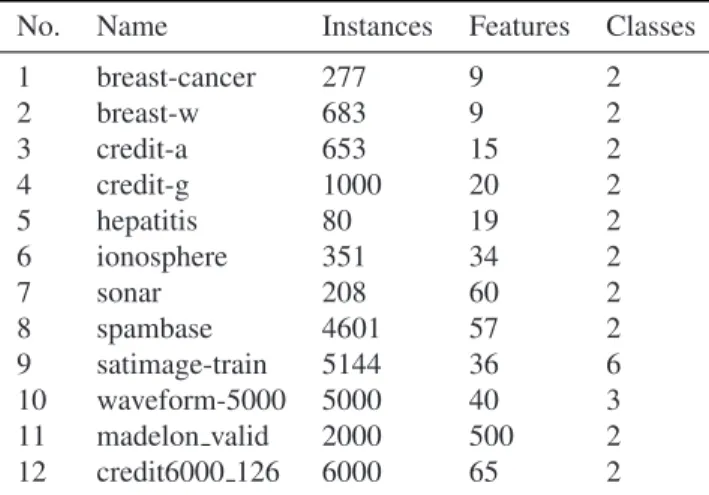
GB main memory. The algorithm proposed in this paper was implemented with Visual Studio 2010 express using programming language C#. Two valuable utilities, MINE package[25] and Aﬃnity Propagation toolkit[27] were adopted during implementation. Other feature selection methods in experiment were constructed under Weka[28] platform which integrates various of data mining elements and algorithms under a uniform framework. The majority of our experimental datasets are from UCI Machine Learning Repository [29]. Most of them are commonly used in machine learning and pattern recognition research. Another dataset from the NIPS 2003 feature selection benchmark is adopted to validate relatively high dimensionality condition. Furthermore, a real world dataset that contains credit information from a bank in China has also been tested in our experiments. Details of these benchmark datasets used in experiments are provided in Table 1.

Table 1. Descriptions of datasets in our experiment

No. Name Instances Features Classes

1 breast-cancer 277 9 2 2 breast-w 683 9 2 3 credit-a 653 15 2 4 credit-g 1000 20 2 5 hepatitis 80 19 2 6 ionosphere 351 34 2 7 sonar 208 60 2 8 spambase 4601 57 2 9 satimage-train 5144 36 6 10 waveform-5000 5000 40 3 11 madelon valid 2000 500 2 12 credit6000 126 6000 65 2

A series of popular feature selection methods were chosen for comparison, that’s Information Gain, Relief[30] and RFE[31]. The reason we use these methods is that they are individual evaluations[32]. That means a weight value could be assigned for each feature. Features could be ranked by this measure and then a speciﬁc number of attributes could be selected from the top of this ranking list.

To show generality of our algorithm, classification prediction capability for features selected are tested with several classical classifiers, i.e. SVM[33] , Naive Bayes[34], C4.5[35], Random Forest[36] and KNN[37]. These classification algorithms are all popular and widely applied in various research fields.

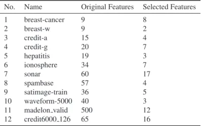
For simplicity reason, median value was chosen as thepreferenceparameter and our method were applied on the datasets. Table 2 has showed the number of features selected through our algorithm. Next, other three feature selection method were used to generate the same number of features.

After that, classiﬁcation problem was validation through four classical classiﬁers. The accuracy results of these methods on the features selected data were showed in Table 3, 4, 5 and 6. In each table, ‘NoSelection’ and ‘MICAP’ columns exhibit the result of no selection and our algorithm. And columns ‘IG’, ‘Relief’ and ‘RFE’ stand for the result of Information Gain, Relief[30] and RFE[31] these three feature selection algorithms respectively.

To make the result more clear, we grouped the classification result for the same dataset and classifier. The packed results were illustrated in figure 1, 2, 3 and 4 respectively. Each figure represents the classification result for one classifier and each group stands for one dataset indexed by number. The leftmost bar shows the situation without any feature selection procedure. The second bar from left show the performance of our algorithm. By comparing with other four bars in the figure, we can find that for most datasets our algorithm is comparable with original data and other three feature selection methods. Especially for dataset ‘satimage-train’ our method outperforms other methods under all four classifiers. Moreover, for one of the NIPS 2003 dataset ‘madelon valid’, our unsupervised method achieves better result than original dataset which reveals the capability of discovering the nature of data. For our own bank credit dataset ‘credit6000 126’, our method also shows its competence for real world application.

(6)

Table 2. Number of features selected by our algorithm with the median value as preference

No. Name Original Features Selected Features

1 breast-cancer 9 8 2 breast-w 9 2 3 credit-a 15 4 4 credit-g 20 7 5 hepatitis 19 3 6 ionosphere 34 7 7 sonar 60 17 8 spambase 57 4 9 satimage-train 36 5 10 waveform-5000 40 3 11 madelon valid 500 12 12 credit6000 126 65 16

Table 3. Naive Bayes classiﬁcation accuracy for original data and four feature selection methods

Name NoSelection MICAP IG Relief RFE

breast-cancer 0.733 0.729 0.729 0.729 0.729 breast-w 0.962 0.937 0.949 0.947 0.950 credit-a 0.775 0.730 0.743 0.864 0.741 credit-g 0.888 0.775 0.900 0.875 0.900 hepatitis 0.826 0.883 0.877 0.915 0.895 ionosphere 0.668 0.663 0.663 0.697 0.702 sonar 0.795 0.632 0.787 0.687 0.807 spambase 0.756 0.743 0.748 0.723 0.757 satimage-train 0.797 0.781 0.761 0.569 0.776 waveform-5000 0.801 0.737 0.650 0.664 0.751 madelon valid 0.542 0.602 0.613 0.617 0.630 credit6000 126 0.693 0.741 0.722 0.696 0.692

Table 4. C4.5 classiﬁcation accuracy for original data and four feature selection methods

(7)

Table 5. Random Forest classiﬁcation accuracy for original data and four feature selection methods

Table 6. K Nearest Neighbors classiﬁcation accuracy for original data and four feature selection methods

(8)

Fig. 2. Comparison of diﬀerent feature selection methods on C4.5 classiﬁer

(9)

Fig. 4. Comparison of diﬀerent feature selection methods on KNN classiﬁer

5. Conclusion and Future work

Feature selection based on relevance of attributes is an old topic. However, fresh relationship measure between variables gives the concept “relevance” new meanings. In this paper, we follow the idea of attributes clustering, and propose a new unsupervised feature selection method combining two state-of-the-art discovering, e.t. maximal information coefficient and affinity propagation clustering method. Maximal information coefficient[23] is an powerful measure for relevance. Affinity propagation cluster instances based their nature relationship[26]. We integrate these method together and take some data experiments. Simulation results show that our unsupervised feature selection algorithm is comparable with the classical supervised feature selection methods in experiments. In some cases, our unsupervised way even outperform the supervised way!

It probably results from the fact that our method takes the advantages of the two sophisticated methods. Our algorithm take no account of supervised information. In fact, label information could help us improve the perfor-mance and the understanding of data mining task. Therefore, how to make our method beneﬁt from supervised learning procedure will be our future work.

6. Acknowledgments

The authors thanks the anonymous reviewers for his or her careful reading and valuable comments. This work was partially supported by the the National Natural Science Foundation of China(Grant No. 70921061, 11271361, 71201143, 61003167), the CAS/SAFEA International Partnership Program for Creative Research Teams, Major International (Region) Joint Research Project (No.71110107026).

References

[1] U. Fayyad, G. Piatetsky-Shapiro, P. Smyth, From data mining to knowledge discovery in databases, AI magazine 17 (3) (1996) 37. [2] H. Liu, J. Sun, L. Liu, H. Zhang, Feature selection with dynamic mutual information, Pattern Recognition 42 (7) (2009) 1330–1339. [3] S. Roweis, L. Saul, Nonlinear dimensionality reduction by locally linear embedding, Science 290 (5500) (2000) 2323–2326.

[4] S. Phdikar, J. Sil, A. Das, Feature selection by attribute clustering of infected rice plant images, International Journal of Machine Intelligence 3 (2) (2011) 74–88.

[5] I. Guyon, A. Elisseeﬀ, An introduction to variable and feature selection, Journal of Machine Learning Research 3 (2003) 1157–1182. [6] J. Li, Z. Chen, L. Wei, W. Xu, G. Kou, Feature selection via least squares support feature machine, International Journal of Information

(10)

[7] Z. Chen, J. Li, L. Wei, A multiple kernel support vector machine scheme for feature selection and rule extraction from gene expression data of cancer tissue, Artiﬁcial Intelligence in Medicine 41 (2) (2007) 161–175.

[8] I. Dhillon, S. Mallela, R. Kumar, A divisive information theoretic feature clustering algorithm for text classiﬁcation, Journal of Machine Learning Research 3 (2003) 1265–1287.

[9] T. Hong, P. Wang, Y. Lee, An eﬀective attribute clustering approach for feature selection and replacement, Cybernetics and Systems: An International Journal 40 (8) (2009) 657–669.

[10] S. Zhu, D. Wang, K. Yu, T. Li, Y. Gong, Feature selection for gene expression using model-based entropy, IEEE/ACM Transactions on Computational Biology and Bioinformatics 7 (1) (2010) 25–36.

[11] P. Ravisankar, V. Ravi, G. Raghava Rao, I. Bose, Detection of ﬁnancial statement fraud and feature selection using data mining tech-niques, Decision Support Systems 50 (2) (2011) 491–500.

[12] Y. Tian, Y. Shi, X. Liu, Recent advances on support vector machines research, Technological and Economic Development of Economy 18 (1) (2012) 5–33.

[13] Z. Qi, Y. Xu, L. Wang, Y. Song, Online multiple instance boosting for object detection, Neurocomputing 74 (10) (2011) 1769–1775. [14] Z. Qi, Y. Tian, S. Yong, Robust twin support vector machine for pattern classiﬁcation, Pattern Recognition 46(1) (2013) 305–316.

doi:doi:10.1016/j.patcog.2012.06.019.

[15] I. Rodriguez-Lujan, R. Huerta, C. Elkan, C. Cruz, Quadratic programming feature selection, Journal of Machine Learning Research 11 (2010) 1491–1516.

[16] W. Au, K. Chan, A. Wong, Y. Wang, Attribute clustering for grouping, selection, and classiﬁcation of gene expression data, IEEE_/ACM Transactions on Computational Biology and Bioinformatics 2 (2) (2005) 83–101.

[17] F. Pereira, N. Tishby, L. Lee, Distributional clustering of english words, in: Proceedings of the 31st Annual Meeting on Association for Computational Linguistics, 1993, pp. 183–190.

[18] N. Tishby, F. Pereira, W. Bialek, The information bottleneck method, in: Proceedings of the 37th Annual Allerton Conference on Communication, Control and Computing, 1999, pp. 368–377.

[19] L. Baker, A. McCallum, Distributional clustering of words for text classiﬁcation, in: Proceedings of the 21st Annual international ACM SIGIR conference on Research and development in information retrieval, ACM, 1998, pp. 96–103.

[20] J. Jiang, R. Liou, S. Lee, A fuzzy self-constructing feature clustering algorithm for text classiﬁcation, IEEE Transactions on Knowledge and Data Engineering 23 (3) (2011) 335–349.

[21] E. Amaldi, V. Kann, On the approximability of minimizing nonzero variables or unsatisﬁed relations in linear systems, Theoretical Computer Science 209 (1) (1998) 237–260.

[22] E. Combarro, E. Montanes, I. Diaz, J. Ranilla, R. Mones, Introducing a family of linear measures for feature selection in text categoriza-tion, IEEE Transactions on Knowledge and Data Engineering 17 (9) (2005) 1223–1232.

[23] D. Reshef, Y. Reshef, H. Finucane, S. Grossman, G. McVean, P. Turnbaugh, E. Lander, M. Mitzenmacher, P. Sabeti, Detecting novel associations in large data sets, Science 334 (6062) (2011) 1518–1524.

[24] Supporting online material for “detecting novel associations in large data sets”,http://www.sciencemag.org/cgi/content/full/

334/6062/1518/DC1.

[25] MINE software package,http://exploredata.net.

[26] B. Frey, D. Dueck, Clustering by passing messages between data points, Science 315 (5814) (2007) 972–976. [27] Aﬃnity Propagation software package,http://www.psi.toronto.edu/index.php?q=affinitypropagation.

[28] M. Hall, E. Frank, G. Holmes, B. Pfahringer, P. Reutemann, I. H. Witten, The weka data mining software: an update, SIGKDD Explor. Newsl. 11 (1) (2009) 10–18.

[29] A. Frank, A. Asuncion, UCI machine learning repository,http://archive.ics.uci.edu/ml, university of California, Irvine, School of Information and Computer Sciences (2010).

[30] K. Kira, L. A. Rendell, A practical approach to feature selection, in: Ninth International Workshop on Machine Learning, Morgan Kaufmann, 1992, pp. 249–256.

[31] I. Guyon, J. Weston, S. Barnhill, V. Vapnik, Gene selection for cancer classiﬁcation using support vector machines, Machine Learning 46 (2002) 389–422.

[32] L. Yu, H. Liu, Eﬃcient feature selection via analysis of relevance and redundancy, Journal of Machine Learning Research 5 (2004) 1205–1224.

[33] C.-C. Chang, C.-J. Lin, LIBSVM: A library for support vector machines, ACM Transactions on Intelligent Systems and Technology 2 (2011) 27:1–27:27, software available athttp://www.csie.ntu.edu.tw/~cjlin/libsvm.

[34] G. H. John, P. Langley, Estimating continuous distributions in bayesian classiﬁers, in: Eleventh Conference on Uncertainty in Artiﬁcial Intelligence, 1995, pp. 338–345.

[35] G. Webb, Decision tree grafting from the all-tests-but-one partition, Morgan Kaufmann, San Francisco, CA, 1999. [36] L. Breiman, Random forests, Machine Learning 45 (1) (2001) 5–32.